Survival Probabilities in Coherent Exciton Transfer with Trapping

Abstract

In the quest for signatures of coherent transport we consider exciton trapping in the continuous-time quantum walk framework. The survival probability displays different decay domains, related to distinct regions of the spectrum of the Hamiltonian. For linear systems and at intermediate times the decay obeys a power-law, in contrast to the corresponding exponential decay found in incoherent continuous-time random walk situations. To differentiate between the coherent and incoherent mechanisms, we present an experimental protocol based on a frozen Rydberg gas structured by optical dipole traps.

Recent years have seen an upsurge of interest in coherent energy transfer, given the experimental advances in manipulating and controlling quantum mechanical systems. From the theoretical side, such investigations are of long standing; see, e.g., Ziman (1972). Here, tight-binding models, which model coherent exciton transfer, are closely related to the quantum walks (QW). As their classical random walk (RW) counterpart, QW appear in two variants: discrete-time QW Aharonov et al. (1993) and continuous-time QW (CTQW) Farhi and Gutmann (1998). Experimental implementations have only recently been proposed for both QW variants, based, e.g., on microwave cavities Sanders et al. (2003), ground state atoms Dür et al. (2002) or Rydberg atoms Côté et al. (2006) in optical lattices, or the orbital angular momentum of photons Zhang et al. (2007).

An appropriate means to monitor transport is to follow the decay of the excitation due to trapping. The long time decay of chains with traps is a well studied problem for classical systems Klafter and Silbey (1980); Grassberger and Procaccia (1982): for an ensemble of chains of different length with traps at both ends the averaged exciton survival probability has a stretched exponential form $\exp(-bt^{\lambda})$, with $\lambda=1/3$ (see, e.g., Grassberger and Procaccia (1982)). In contrast, quantum mechanical tight-binding models lead to $\lambda=1/4$ Pearlstein (1971); Parris (1989b). However, up to now only little is known about the decay of the quantum mechanical survival probability at experimentally relevant intermediate times.

Here we evaluate and compare the intermediate-time decays due to trapping for both RW and QW situations by employing the similarity of the CTRW and the CTQW formalisms. Without traps, the coherent dynamics of excitons on a graph of connected nodes is modeled by the CTQW, which is obtained by identifying the Hamiltonian ${\bf H}_{0}$ of the system with the CTRW transfer matrix ${\bf T}_{0}$, i.e., ${\bf H}_{0}=-{\bf T}_{0}$; see e.g. Farhi and Gutmann (1998); Mülken and Blumen (2005a) (we will set $\hbar\equiv 1$ in the following). For undirected graphs, ${\bf T}_{0}$ is related to the connectivity matrix ${\bf A}_{0}$ of the graph by ${\bf T}_{0}=-{\bf A}_{0}$, where (for simplicity) all transmission rates are taken to be equal. Thus, in the following we take ${\bf H}_{0}={\bf A}_{0}$. The matrix ${\bf A}_{0}$ has as non-diagonal elements $A^{(0)}_{k,j}$ the values $-1$ if nodes $k$ and $j$ of the graph are connected by a bond and $0$ otherwise. The diagonal elements $A^{(0)}_{j,j}$ of ${\bf A}_{0}$ equal the number of bonds $f_{j}$ which exit from node $j$. By fixing the coupling strength between two connected nodes to $|H^{(0)}_{k,j}|=1$, the time scale is given in units of $[\hbar/H^{(0)}_{k,j}]$. For the Rydberg gases considered in the following, the coupling strength is roughly $H^{(0)}_{k,j}/\hbar\gtrsim 1$ MHz, i.e., the time unit for transfer between two nodes is of the order of a few hundred nanoseconds.

The states $|j\rangle$ associated with excitons localized at the nodes $j$ ($j=1,\dots,N$) form a complete, orthonormal basis set (COBS) of the whole accessible Hilbert space, i.e., $\langle k|j\rangle=\delta_{kj}$ and $\sum_{k}|k~{}\rangle\langle~{}k|={\bf 1}$. In general, the time evolution of a state $|j\rangle$ starting at time $t_{0}=0$ is given by $|j;t\rangle=\exp(-i{\bf H}_{0}t)|j\rangle$; hence the transition amplitudes and the probabilities read $\alpha_{kj}(t)\equiv\langle k|\exp(-i{\bf H}_{0}t)|j\rangle$ and $\pi_{kj}(t)\equiv\left|\alpha_{kj}(t)\right|^{2}$, respectively. In the corresponding classical CTRW case the transition probabilities follow from a master equation as $p_{kj}(t)=\langle k|\exp({\bf T}_{0}t)|j\rangle$ Farhi and Gutmann (1998); Mülken and Blumen (2005a).

Consider now that out of the $N$ nodes $M$ are traps with $M\leq~{}N$; we denote them by $m$, so that $m\in{\cal M}$, with ${\cal M}\subset\{1,\dots,N\}$. We incorporate trapping into the CTQW formalism phenomenologically by following an approach based on time dependent perturbation theory Pearlstein (1971); Parris (1989b); Sakurai (1994). The new Hamiltonian is ${\bf H}={\bf H}_{0}+i{\bf\Gamma}$, where the trapping operator $i{\bf\Gamma}$ has at the trap nodes $m$ purely imaginary diagonal elements $i\Gamma_{mm}$, which we assume to be equal for all $m$ ($\Gamma_{mm}\equiv\Gamma>0$), and is zero otherwise. As a result, ${\bf H}$ is non-hermitian and has $N$ complex eigenvalues, $E_{l}=\epsilon_{l}-i\gamma_{l}$ ($l=1,\dots,N$). In general, ${\bf H}$ has $N$ left and $N$ right eigenstates $|\Phi_{l}\rangle$ and $\langle\tilde{\Phi}_{l}|$, respectively. For most physically interesting cases the eigenstates can be taken as biorthonormal, $\langle\tilde{\Phi}_{l}|\Phi_{l^{\prime}}\rangle=\delta_{ll^{\prime}}$, and complete, $\sum_{l=1}^{N}|\Phi_{l}\rangle\langle\tilde{\Phi}_{l}|={\bf 1}$; see, e.g., Ref. Sternheim and Walker (1972). Moreover, we have $\langle k|\Phi_{l}\rangle^{*}=\langle\tilde{\Phi}_{l}|k\rangle$. Thus, the transition amplitudes can be calculated as $\alpha_{kj}(t)=\sum_{l}\exp[-\gamma_{l}t]\exp[-i\epsilon_{l}t]\langle k|\Phi_{l}\rangle\langle\tilde{\Phi}_{l}|j\rangle$; here the imaginary parts $\gamma_{l}$ of $E_{l}$ determine the temporal decay of $\pi_{kj}(t)=\left|\alpha_{kj}(t)\right|^{2}$.

In an ideal experiment one would excite exactly one node, say $j\not\in{\cal M}$, and read out the outcome $\pi_{kj}(t)$, i.e., the probability to be at node $k\not\in{\cal M}$ at time $t$. However, it is easier to keep track of the total outcome at all nodes $k\not\in{\cal M}$, namely, $\sum_{k\not\in{\cal M}}\pi_{kj}(t)$. Since the states $|k\rangle$ form a COBS we have $\sum_{k\not\in{\cal M}}|k\rangle\langle k|={\bf 1}-\sum_{m\in{\cal M}}|m\rangle\langle m|$, which leads to:

$$\sum_{k\not\in{\cal M}}\pi_{kj}(t) = \sum_{l=1}^{N}e^{-2\gamma_{l}t}\langle j|\Phi_{l}\rangle\langle\tilde{\Phi}_{l}|j\rangle-\sum_{l,l^{\prime}=1}^{N}e^{-i(E_{l}-E_{l^{\prime}}^{*})t}$$ (1)

$$\times\sum_{m\in{\cal M}}\langle j|\Phi_{l^{\prime}}\rangle\langle\tilde{\Phi}_{l^{\prime}}|m\rangle\langle m|\Phi_{l}\rangle\langle\tilde{\Phi}_{l}|j\rangle.$$

By averaging over all $j\not\in{\cal M}$, the mean survival probability $\Pi_{M}(t)\equiv\frac{1}{N-M}\sum_{j\not\in{\cal M}}\sum_{k\not\in{\cal M}}\pi_{kj}(t)$ is given by

$$\Pi_{M}(t)=\frac{1}{N-M}\sum_{l=1}^{N}e^{-2\gamma_{l}t}\Big{[}1-2\sum_{m\in{\cal M}}\langle\tilde{\Phi}_{l}|m\rangle\langle m|\Phi_{l}\rangle\Big{]}$$

$$+\frac{1}{N-M}\sum_{l,l^{\prime}=1}^{N}e^{-i(E_{l}-E_{l^{\prime}}^{*})t}\Big{[}\sum_{m\in{\cal M}}\langle\tilde{\Phi}_{l^{\prime}}|m\rangle\langle m|\Phi_{l}\rangle\Big{]}^{2}.$$ (2)

For CTRW we include trapping in a formally similar fashion as for the CTQW. Here, however, the classical transfer matrix ${\bf T}_{0}$ is modified by the trapping matrix ${\bf\Gamma}$, such that the new transfer matrix is ${\bf T}={\bf T}_{0}-{\bf\Gamma}$, Lakatos-Lindenberg et al. (1971). For a single linear system with traps at each end, the mean survival probability $P_{M}(t)\equiv\frac{1}{N-M}\sum_{j\not\in{\cal M}}\sum_{k\not\in{\cal M}}p_{kj}(t)$ decays exponentially at intermediate and at long times Lakatos-Lindenberg et al. (1971). As we proceed to show, the decays of $\Pi_{M}(t)$ and $P_{M}(t)$ are very different, thus allowing to distinguish experimentally whether the exciton transfer is coherent or not.

For long $t$ and small $M/N$, Eq. (2) simplifies considerably: At long $t$ the oscillating term on the right hand side drops out and for small $M/N$ we have $2\sum_{m\in{\cal M}}\langle\tilde{\Phi}_{l}|m\rangle\langle m|\Phi_{l}\rangle\ll~{}1$. Thus, $\Pi_{M}(t)$ is mainly a sum of exponentially decaying terms:

$$\Pi_{M}(t)\approx\frac{1}{N-M}\sum_{l=1}^{N}\exp[-2\gamma_{l}t].$$ (3)

Asymptotically, Eq. (3) is dominated by the $\gamma_{l}$ values closest to zero. If the smallest one, $\gamma_{\rm min}$, is well separated from the other values, one is led for $t\gg 1/\gamma_{\rm min}$ to the exponential decay found in earlier works, $\Pi_{M}(t)=\exp(-2\gamma_{\rm min}t)$ Parris (1989b).

Such long times are not of much experimental relevance (see also below), since most measurements highlight shorter times, in which many $\gamma_{l}$ contribute. In the corresponding energy range the $\gamma_{l}$ often scale, as we show in the following, so that in a large $l$ range $\gamma_{l}\sim al^{\mu}$. The prefactor $a$ depends only on $\Gamma$ and $N$ Parris (1989b). For densely distributed $\gamma_{l}$ and at intermediate times one has, from Eq. (3),

$$\Pi_{M}(t)\approx\int dx\ e^{-2atx^{\mu}}=\int dy\ \frac{e^{-y^{\mu}}}{(2at)^{1/\mu}}\sim t^{-1/\mu}.$$ (4)

The envisaged experimental setup consists of clouds of ultra-cold Rydberg atoms assembled in a chain over which an exciton migrates; the trapping of the exciton occurs at the ends of the chain. The dipolar interactions between Rydberg atoms depend on the mutual distance $R$ between the nodes as $R^{-3}$. Now, CTRW over a chain of regularly arranged sites lead both for nearest-neighbor steps and for step distributions depending on $R$ as $R^{-\gamma}$, with $\gamma>3$, to a standard diffusive behavior and, therefore, belong to the same universality class, see e.g. Weiss (1994). The reason is that in one dimension for $\gamma>3$ the first two moments, $\langle R\rangle$ and $\langle R^{2}\rangle$, are finite. Thus, although the quantitative results will differ, the qualitative behavior is similar. Hence, we focus on a nearest-neighbor tight-binding model and consider a chain of length $N$ with two traps ($M=2$) located at its ends ($m=1$ and $m=N$), . The CTQW Hamiltonian thus reads

$${\bf H} = \sum_{n=1}^{N}\Big{(}2|n\rangle\langle n|-|n-1\rangle\langle n|-|n+1\rangle\langle n|\Big{)}$$ (5)

$$+i\Gamma\sum_{m=1,N}|m\rangle\langle m|.$$

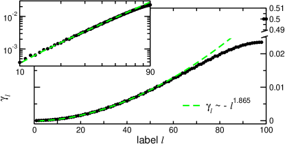
Figure 1: (Color online) Imaginary parts $\gamma_{l}$ (dots) in ascending order for $N=100$ and $\Gamma=1$. Note the shortened $y$ axis. The inset shows $\gamma_{l}$ in log-log scale for $l=10,\dots,90$.

In Fig. 1 we show the spectrum of $\gamma_{l}$ for $N=100$ and $\Gamma=1$; the double logarithmic plot (see inset) demonstrates that scaling holds for $10\leq l\leq 60$, with an exponent of about $\mu=1.865$. In this domain $\gamma_{l}\in[0.0012,0.012]$, which translates to experimentally accessible coherence times of about $10-100\mu$s. For comparison the smallest decay rate is $\gamma_{\rm min}=7.94\times 10^{-6}$, which corresponds to experimentally unrealistic coherence times of the order of tenths of seconds.

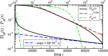
Figure 2: (Color online) Temporal decay of $\Pi_{M}(t)$ (solid black lines) and $P_{M}(t)$ (short dashed green lines) for $N=100$ and $\Gamma=1$ in double logarithmic scales (upper three curves) and in logarithmic scales (lower three curves). Indicated are the fits to $\Pi_{M}(t)$ (long dashed lines) in the intermediate (upper red) and the long (lower blue) time regime.

The corresponding transfer matrix of the classical CTRW reads

$${\bf T} = -\sum_{n=1}^{N}\Big{(}2|n\rangle\langle n|-|n-1\rangle\langle n|-|n+1\rangle\langle n|\Big{)}$$ (6)

$$-\Gamma\sum_{m=1,N}|m\rangle\langle m|.$$

In Fig. 2 we compare the classical $P_{M}(t)$ to the quantum mechanical survival probability $\Pi_{M}(t)$ for a linear system with $N=100$ and $\Gamma=1$. Evidently, $P_{M}(t)$ and $\Pi_{M}(t)$ differ strongly: the $P_{M}(t)$ decay established for CTRW is practically exponential. $\Pi_{M}(t)$, on the other hand, shows two regimes: a power-law decay at intermediate times (upper red curve) and an exponential decay (lower blue curve) at very long times.

We now turn to the parameter dependences of $\Pi_{M}(t)$. Figure 3 displays the dependence of $\Pi_{M}(t)$ on $N$. We note that the scaling regime, where $\Pi_{M}(t)\sim t^{-1/\mu}$, gets larger with increasing $N$. The cross-over to this scaling region from the domain of short times occurs around $t\approx N/2$. For larger $N$ and in the intermediate time domain $\Pi_{M}(t)$ scales nicely with $N$. In this case, the power-law approximation [Eq. (4)] holds and by rescaling $l$ to $l/N$ we get from Eq. (3) that

$$\Pi_{M}(t)\sim\sum_{l}e^{-2N^{-3}l^{\mu}t}=\sum_{l}\exp\Big{[}-2(l/N)^{\mu}N^{-(3-\mu)}t\Big{]},$$ (7)

where we used that $a\sim N^{-3}$ for a linear system Parris (1989b). Thus when rescaling $l$ to $l/N$, time has to be rescaled by the factor $N^{-(3-\mu)}$. Indeed, all curves where a power-law behavior can be justified fall on a master curve; see the inset in Fig. 3.

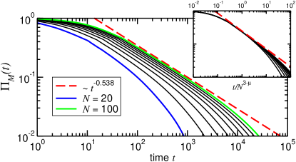
Figure 3: (Color online) $N$-dependence of $\Pi_{M}(t)$ for $\Gamma=1$; $N$ increases in steps of $10$ from $20$ (blue line) to $100$ (green line). The inset shows $\Pi_{M}(t)$ versus the rescaled time $t/N^{3-\mu}$.

The temporal decay does not only depend on $N$ but also on $\Gamma$. Figure 4 shows $\Pi_{M}(t)$ for $N=50$ and different $\Gamma$. For values $\Gamma\gg 1$ (green lines) and $\Gamma\ll 1$ (black lines) the curves shift to longer times. Values of $\Gamma$ close to $1$ (blue lines) lead to the quickest decay. Note that these values are of the same order as the coupling strength between the non trap nodes, $H_{j,j\pm 1}=-1$.

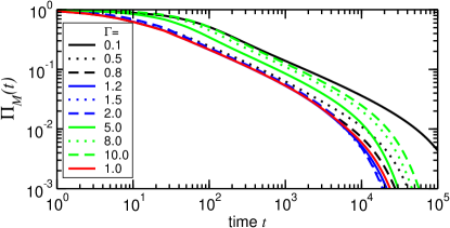
Figure 4: (Color online) $\Gamma$-dependence of $\Pi_{M}(t)$ for intermediate $t$ and $N=50$.

An experimental implementation of the described system has to meet several criteria. A single node must represent a well-defined two-level system to ensure coherent energy transfer while at the same time a mechanism is needed to trap an exciton with a controllable trapping efficiency. Furthermore, the chain must be static with negligible motion and should allow for spatially selective excitation and detection of the exciton. These demands rule out many possible candidates for an experimental realization of CTQW. A frozen Rydberg gas [17] can meet all of the above demands by combining the rich internal structure of highly excited atoms whith the full quantum control over the external degrees of freedom that is available in up-to-date experiments with ultracold atoms. The internal structure of Rydberg atoms provides both decoupled two-level subsystems and tunable traps, while the pronounced Stark shift allows to selectively address single sites in a chain when an electric field gradient is applied. At the same time, experimentally accessible temperatures below 1$\,\mu$K ensure that the thermal motion is negligible.

Our scheme starts from a cloud of laser-cooled ground state atoms prepared in a chain of optical dipole traps Grimm et al. (2000). Each site represents one node with distances between sites of 5 to 20 $\mu$m. For an experimentally achievable extension of 1 mm this translates into approximately 100 nodes. All nodes are excited to Rydberg states exploiting the dipole blockade mechanism to ensure a single Rydberg excitation per node Lukin et al. (2001) which avoids many-body effects Anderson et al. (2002). A two-level system is realized by a transition between energetically isolated states, i.e., by low-angular-momentum states which exhibit a large quantum defect, e.g., $\textsf{n}\textrm{S}\;\rightleftharpoons\;\textsf{n}\textrm{P}\;$. A number of experiments has revealed the coherent character of this process Anderson et al. (2002). By contrast to low-$\ell$ states, states with angular momenta $\ell\geq 3$ have no quantum defect and are degenerate. This allows to construct an exciton trap with the transitions $\textsf{n}^{\prime}\textrm{D}\;\rightleftharpoons\;\textsf{n}^{\prime\prime}\textrm{F}\xrightarrow{\mathrm{rf}}\;\textsf{n}^{\prime\prime}\ell(\ell\geq 3)$, where the first transition is the dipole transition providing the coupling to neighboring nodes while the second transition, driven by a radio-frequency (rf) field, represents the trap and decouples this site from the energy transfer, as the large degeneracy of the high-$\ell$ states ensures an efficient suppression of the coupling back to the $\textsf{n}^{\prime\prime}$F state . By changing the strength of the driving rf field, the trapping efficiency can be tuned. The population of the $\textsf{n}^{\prime\prime}\ell$ state is directly proportional to $1-\Pi_{M}(t)$ and can be determined by state selective field ionization Gallagher (1994). In an experiment the central nodes would be prepared in the S state and the trap nodes in the D state. A single S node is swapped to P through a microwave transition in an electric field gradient which makes the resonance S$\rightarrow$P position sensitive. This is equivalent to exciting a single exciton. The energy transport is started by removing the field gradient making the transition energy the same for all nodes.

There are two important decoherence mechanisms which are given by the spontaneous decay of the involved Rydberg states and by the atomic motion. Exemplarily, for the 71S and 61D states of rubidium and a distance of 20$\mu$m between nodes we calculate a transfer time of $\tau=$145 ns between two neighboring sites, radiative lifetimes including black-body radiation of $\geq$100 $\mu$s and residual thermal motion that leads to a change of the interatomic distance of 1.4 $\mu$m per 100 $\mu$s at a temperature of 1 $\mu$K. Another source of decoherence is the interaction-induced motion Li et al. (2005). We can model this motion quantitatively Amthor et al. (2007) and calculate negligible changes of the interatomic distances of less than 0.2 $\mu$m per 100 $\mu$s. This means that both the chain and the elementary atomic system sustain coherence over timescales on the order of several ten $\mu$s and longer.

In conclusion, we have identified different time domains in the CTQW exciton decay in the presence of traps, domains which are directly related to the complex spectrum of the system’s Hamiltonian. The CTQW average survival probability $\Pi_{M}(t)$ for an exciton to stay inside a linear system of $N$ nodes with traps at each end can clearly be distinguished from its classical CTRW counterpart, $P_{M}(t)$. Finally, we proposed an experimental test for coherence on the basis of ultra-cold Rydberg atoms.

We gratefully acknowledge support from the Deutsche Forschungsgemeinschaft (DFG), the Ministry of Science, Research and the Arts of Baden-Württemberg (AZ: 24-7532.23-11-11/1) and the Fonds der Chemischen Industrie.

References

- Ziman (1972) J. M. Ziman, Principles of the Theory of Solids (Cambridge University Press, Cambridge, England, 1972).
- Aharonov et al. (1993) Y. Aharonov, L. Davidovich, and N. Zagury, Phys. Rev. A 48, 1687 (1993); J. Kempe, Contemporary Physics 44, 307 (2003).
- Farhi and Gutmann (1998) E. Farhi and S. Gutmann, Phys. Rev. A 58, 915 (1998).
- Sanders et al. (2003) B. C. Sanders et al., Phys. Rev. A 67, 042305 (2003).
- Dür et al. (2002) W. Dür et al., Phys. Rev. A 66, 052319 (2002).
- Côté et al. (2006) R. Côté et al., New J. Phys. 8, 156 (2006).
- Zhang et al. (2007) P. Zhang, et al., Phys. Rev. A 75, 052310 (2007).
- Klafter and Silbey (1980) J. Klafter and R. Silbey, J. Chem. Phys. 72, 849 (1980); ibid. 74, 3510 (1981).
- Grassberger and Procaccia (1982) P. Grassberger and I. Procaccia, J. Chem. Phys. 77, 6281 (1982); R. F. Kayser and J. B. Hubbard, Phys. Rev. Lett. 51, 79 (1983); G. Forgacs, D. Mukamel, and R. A. Pelcovits, Phys. Rev. B 30, 205 (1984).
- Pearlstein (1971) R. M. Pearlstein, J. Chem. Phys. 56, 2431 (1971); D. L. Huber, Phys. Rev. B 22, 1714 (1980); 45, 8947 (1992); P. E. Parris, Phys. Rev. Lett. 62, 1392 (1989a); V. A. Malyshev, R. Rodríguez, and F. Domínguez-Adame, J. Lumin. 81, 127 (1999).
- Parris (1989b) P. E. Parris, Phys. Rev. B 40, 4928 (1989b).
- Mülken and Blumen (2005a) O. Mülken and A. Blumen, Phys. Rev. E 71, 016101 (2005a); ibid. 71, 036128 (2005); ibid. 73, 066117 (2006b).
- Sakurai (1994) J. Sakurai, Modern Quantum Mechanics (Addison-Wesley, Redwood City, CA, 1994), 2nd ed., p. 342ff.
- Sternheim and Walker (1972) M. M. Sternheim and J. F. Walker, Phys. Rev. C 6, 114 (1972).
- Lakatos-Lindenberg et al. (1971) K. Lakatos-Lindenberg, R. P. Hemenger, and R. M. Pearlstein, J. Chem. Phys. 56, 4852 (1971); F. Domínguez-Adame, E. Maciá, and A. Sánchez, Phys. Rev. B 51, 878 (1995).
- Weiss (1994) G. H. Weiss, Aspects and Applications of the Random Walk (North-Holland, Amsterdam, 1994), p. 78ff; J. Klafter et al., Phys. Rev. A 35, 3081 (1987), Eqs. (25)-(27).
- Anderson et al. (1998) W. R. Anderson, J. R. Veale, and T. F. Gallagher, Phys. Rev. Lett. 80, 249 (1998); I. Mourachko et al., ibid. 80, 253 (1998).
- Grimm et al. (2000) R. Grimm, M. Weidemüller, and Y. B. Ovchinnikov, Adv. At. Mol. Opt. Phys. 42, 95 (2000).
- Lukin et al. (2001) M. D. Lukin et al., Phys. Rev. Lett. 87, 037901 (2001).
- Anderson et al. (2002) W. R. Anderson et al., Phys. Rev. A 65, 063404 (2002); M. Mudrich et al., Phys. Rev. Lett. 95, 233002 (2005); S. Westermann et al., Eur. Phys. J. D 40, 37 (2006).
- Gallagher (1994) T. F. Gallagher, Rydberg Atoms (Cambridge University Press, Cambridge, 1994).
- Li et al. (2005) W. Li, P. J. Tanner, and T. F. Gallagher, Phys. Rev. Lett. 94, 173001 (2005).
- Amthor et al. (2007) T. Amthor et al., Phys. Rev. Lett. 98, 023004 (2007).