Anomalous escape governed by thermal $1/f$ noise

Abstract

We present an analytic study for subdiffusive escape of overdamped particles out of a cusp-shaped parabolic potential well which are driven by thermal, fractional Gaussian noise with a $1/\omega^{1-\alpha}$ power spectrum. This long-standing challenge becomes mathematically tractable by use of a generalized Langevin dynamics via its corresponding non-Markovian, time-convolutionless master equation: We find that the escape is governed asymptotically by a power law whose exponent depends exponentially on the ratio of barrier height and temperature. This result is in distinct contrast to a description with a corresponding subdiffusive fractional Fokker-Planck approach; thus providing experimentalists an amenable testbed to differentiate between the two escape scenarios.

The theme of anomalous sub-diffusion and rate kinetics continuous to flourish over the last years. This topic is driven by the availability of a wealth of intriguing experimental data, ranging from anomalous diffusion in amorphous materials, quantum dots, protein dynamics, actin networks, and biological cells Scher ; Austin ; metzler2000 ; Sokolov ; TangMarcus ; Yang ; Xie2 ; actin ; Caspi ; cell ; PRE04 . Suitable theoretical descriptions derive from continuous time random walks (CTRW) Scher ; Weiss , the CTRW-based fractional Fokker-Planck (FFP)-approach MetzlerPRL ; PRE06 , or the generalized Langevin equation (GLE) HTB90 ; Bao2006 . The GLE-subdiffusion implies power-law-correlated thermal forces (or fractional Gaussian noise (fGn) Mandelbrot ) possessing infinite memory with a $1/\omega^{1-\alpha}$ power spectrum Kupferman ; Xie2 . Such random forces emerge when coupling the system to sub-Ohmic thermal baths with spectral densities $J(\omega)\propto\omega^{\alpha},\;0<\alpha<1$ Bao2006 .

Recent experiments on anomalous conformational subdiffusion in electron-transferring proteins have been successfully modeled within a FFP equation Yang . Soon after, however, the fGn-Langevin approach has been shown to describe the experimental data even more convincingly Xie2 . Both approaches are consistent with molecular dynamics simulations moldyn . In addition, both schemes are consistent with the laws of thermodynamics. Fundamental differences manifest themselves, however, when one considers the escape dynamics. The description of fGn-driven escape presents a long-standing, timely problem. This is so because this complexity, in contrast to the Kramers escape dynamics HTB90 , then generally no longer allows for a detailed, even approximate solution. Recent attempts to solve this challenge can be found in Refs. new , although not yielding a proper solution. Thus, the issue of 1/f-noise driven escape remains an intriguing open problem which continues to haunt the literature.

Our analytic work deals with the unique, but exactly solvable challenge of an escape driven by 1/f-noise out of a cusp-shaped parabolic potential. In doing so we demonstrate that the resulting escape dynamics is scale-free, i.e. it is governed by a power law. This in turn invalidates a rate description. Moreover, the escape dynamics within the fGn-Langevin description is exponentially sensitive to temperature. This result is in marked contrast to the description within a FFP-dynamics which instead yields a temperature-independent power law exponent. Thus, in contrast to the finite mean first passage time (MFPT) result in new our main result exhibits an infinite MFPT, being consistent with a strict subdiffusive escape dynamics. A rate description emerges only when invoking a physically plausible low frequency regularization of the noise spectrum.

GLE-approach. We start out from the GLE for a particle of mass $m$ moving in the potential $V(x)$ HTB90 ; i.e.,

$$m\ddot{x}+\int_{0}^{t}\eta(t-t^{\prime})\dot{x}(t^{\prime})dt^{\prime}+V^{\prime}(x)=\xi(t).$$ (1)

The autocorrelation function $\langle\xi(t)\xi(t^{\prime})\rangle$ of thermal Gaussian noise $\xi(t)$ and the frictional kernel $\eta(t)$ are related by the usual fluctuation-dissipation relation HTB90 :

$$\langle\xi(t)\xi(t^{\prime})\rangle=k_{B}T\eta(|t-t^{\prime}|).$$ (2)

In the following we consider the overdamped limit with $m\to 0$; i.e. the velocity is thermally relaxed at each instant of time. Moreover, we assume that the particles are initially localized in a metastable parabolic well at $x_{0}$, cf. the inset in Fig. (1). The starting probability density then is $P(x,t=0)=\delta(x-x_{0})$. The corresponding non-Markovian master equation for $P(x,t)$ for this GLE is generally not known: For arbitrary physical memory-friction $\eta(t)$ this task is known for two cases only; namely (i) a linear potential $V(x)=-F_{0}\;x$, including the case of free diffusion, i.e. $F_{0}=0$ and (ii) a parabolic potential $V(x)=\kappa x^{2}/2$. The procedure to obtain the master equation is well known: It is solely rooted in the Gaussian nature of $x(t)$ Adelman ; HanggiOld ; HanggiMojtabai ; Hynes ; Kupferman . The result is a time-convolutionless master equation for $P(x,t)$ obeying a Fokker-Planck form with a time-dependent diffusion coefficient $D(t)$ HanggiOld ; Hynes , reading

$$\frac{\partial P(x,t)}{\partial t}=D(t)\frac{\partial}{\partial x}\left(e^{-\beta V(x)}\frac{\partial}{\partial x}e^{\beta V(x)}P(x,t)\right).$$ (3)

Here, $\beta=1/(k_{B}T)$. Notably, $D(t)$ does not depend on $x_{0}$, but is dependent on $V(x)$ and memory friction $\eta(t)$. For a quadratic potential, it can be expressed via the relaxation function $\theta(t)$ of position fluctuations as HanggiOld ; Hynes

$$D(t)=-l_{T}^{2}\frac{d}{dt}\ln\theta(t)\;,$$ (4)

where $l_{T}=\sqrt{k_{B}T/\kappa}$ is the length scale of thermal fluctuations. The Laplace-transform of $\theta(t)$ is related to the memory friction $\eta(t)$ by $\tilde{\theta}(s)=\tilde{\eta}(s)/[\kappa+s\tilde{\eta}(s)]\;$.

We next use a power-law friction kernel $\eta(t)$, reading

$$\eta(t)=\frac{\eta_{\alpha}}{\Gamma(1-\alpha)}\frac{1}{|t|^{\alpha}}\;,\;0<\alpha<1\;.$$ (5)

This friction $\eta(t)$ yields an anomalous, free ($V(x)=0$) subdiffusion with $\langle\delta x^{2}(t)\rangle=2K_{\alpha}t^{\alpha}/\Gamma(1+\alpha)$, where the anomalous diffusion coefficient $K_{\alpha}=k_{B}T/\eta_{\alpha}$ obeys a generalized Einstein relation. For a parabolic potential this yields the relaxation function

$$\theta(t)=E_{\alpha}[-(t/\tau_{D})^{\alpha}]\;,$$ (6)

where $\tau_{D}=(\eta_{\alpha}/\kappa)^{1/\alpha}$, and $E_{\alpha}(z)$ is the Mittag-Leffler function, i.e., $E_{\alpha}(z)=\sum_{n=0}^{\infty}z^{n}/\Gamma(\alpha n+1)$ GorenfloMainardi . It corresponds to the Cole-Cole model of glassy dielectric media Hilfer , whereas the limit $\alpha\to 1$ corresponds to an exponential relaxation with $E_{1}(x)=\exp(x)$.

The thermal fGn $\xi(t)$ is the time derivative of fractional Brownian motion (fBm) Mandelbrot with a power spectrum, $S_{\xi}(\omega)=2k_{B}T\eta_{\alpha}\sin(\pi\alpha/2)/\omega^{1-\alpha}$. For this thermal fGn the GLE in (1) with $m=0$ can formally identically be recast as the ”fractional” Langevin equation, i.e., $\eta_{\alpha}D^{\alpha}_{*}x(t)+V^{\prime}(x)=\xi(t)$, wherein $D_{*}^{\alpha}x(t)=(1/\Gamma(1-\alpha))\int_{0}^{t}\mathrm{d}t^{\prime}(t-t^{\prime})^{-\alpha}\dot{x}(t^{\prime})$ is the operator of the fractional Caputo derivative GorenfloMainardi .

FFP-approach. Alternatively, if instead of the fGn dwelling in a potential in (1), (2), (5) we use a modeling in terms of an overdamped, fractional Fokker-Planck equation description MetzlerPRL ; PRE06 , the probability density obeys

$$D_{*}^{\alpha}P(x,t)=K_{\alpha}\frac{\partial}{\partial x}\left(e^{-\beta V(x)}\frac{\partial}{\partial x}e^{\beta V(x)}P(x,t)\right)\;.$$ (7)

This result derives from an underlying continuous time random walk description of subdiffusion Scher . It as well has an associated Langevin equation in a random operational time $t(\tau)$ Stanislavsky which, however, is profoundly different from the GLE.

Subdiffusive dynamics dwelling in a parabolic potential. The time-convolutionless master equation (3) of the GLE in (1), (2), (5) can be solved exactly for a parabolic potential remark2 : We first transform $P(x,t)$ as $P(x,t)=\exp(-\beta V(x)/2)W(x,t)$ and separate the variables, $W(x,t)=Y(x)\Phi(t)$. For the coordinate-dependent part this yields a spectral representation, reading

$$Y^{{}^{\prime\prime}}_{n}(x)+\frac{\beta}{2}\kappa\left(1-\frac{\beta}{2}\kappa x^{2}+2\lambda_{n}/(\beta\kappa)\right)Y_{n}(x)=0,$$ (8)

where $\lambda_{n}$ and $Y_{n}(x)$ are the corresponding spectral eigenvalues and eigenfunctions. The functions $\Phi_{n}(t)$ obey:

$$\dot{\Phi}_{n}(t)=-\lambda_{n}D(t)\Phi_{n}(t).$$ (9)

By use of (4) the exact solutions of (9) read

$$\Phi_{n}(t)=[\theta(t)]^{s_{n}},$$ (10)

where $s_{n}:=l_{T}^{2}\lambda_{n}$. These findings yield for the explicit solution for the probability density $P(x,t)$ the result,

$$P(x,t)=\exp(-\beta\kappa x^{2}/4)\sum_{n}c_{n}Y_{n}(x)[\theta(t)]^{s_{n}},$$ (11)

where the expansion coefficients $c_{n}$ are determined from the initial probability density $P(x,t=0)$. The spectrum reads $s_{n}=n$, $n=0,1,2,...$. Moreover, the functions $Y_{n}(x)$ are given in terms of Hermite functions HTB90 . The dynamics of the probability evolution is thus ruled by the relaxation function $\theta(t)$ in Eq. (6). Remarkably, the relaxation of the mean value $\langle x(t)\rangle$ follows precisely to the same law as in the case of a FFP description MetzlerPRL . This is surprising because the general solution $P(x,t)$ differs markedly from that of the FFP equation in MetzlerPRL . The solution in the latter case is obtained from (11) by substituting therein $E_{\alpha}[-n(t/\tau_{D})^{\alpha}]$ for $(E_{\alpha}[-(t/\tau_{D})^{\alpha}])^{n}$ within $\theta^{n}(t)$. This follows from the fact that for the FFP in (7), equation (9) is replaced by $D_{*}^{\alpha}\Phi_{n}(t)=-\lambda_{n}K_{\alpha}\Phi_{n}(t)$ MetzlerPRL .

Because the integral over $\theta(t)$ in Eq. (6) is not finite, the statistical mean of random escape times is subject to a divergence, thus invalidating a rate description. Because inter-well transitions can always be broken up into the two steps, i.e. (i) reaching the barrier region from well bottom and (ii) a barrier (re)-crossing to an adjacent well, this implies as well a diverging MFPT when considering more generic situations as the stylized one addressed next.

Escape out of parabolic cusp potential. Let us impose next an infinitely sharp potential cutoff at $x_{a}=L\gg l_{T}$, see the inset in Fig. 1. This sharp cut-off is identical to an absorbing boundary condition, satisfying $P(x,t)=0$ for $x\geq L$. The Gaussian approximation for the GLE therefore remains valid inside the parabolic cusp potential newremark . The solution of eq. (3) for the corresponding boundary value problem now reads anew (for $-\infty<x\leq L$):

$$Y_{n}(x)=U\left(-s_{n}-\frac{1}{2},-x/l_{T}\right)\;,$$ (12)

where $U(\nu,x)$ denotes the parabolic cylinder function. The spectrum for this case reads $\lambda_{n}=s_{n}/l_{T}^{2}$, being determined by the solutions of transcendental equation

$$U\left(-s_{n}-\frac{1}{2},-L/l_{T}\right)=0.$$ (13)

For $L\to\infty$, $s_{n}$ approaches again $n$. For large $L\gg l_{T}$ the decay of the survival probability inside the well $P_{\rm SP}(t)=\int_{-\infty}^{L}P_{\rm cusp}(x,t)dx$ is ruled by the lowest eigenvalue; i.e.,

$$P_{\rm SP}(t)\approx[\theta(t)]^{s_{0}}.$$ (14)

This constitutes our first central result. The value $s_{0}$ is given by the numerical solution of Eq. (13). Remarkably, it is well approximated by the inverse of the properly scaled mean first passage time of the corresponding, memoryless Markovian problem yielding, cf. in Ref. HTB90 :

$$s_{0}^{-1}=l_{T}^{-2}\int_{0}^{L}dy\int_{-\infty}^{y}dx\exp(\beta[V(y)-V(x)]).$$ (15)

This yields $s_{0}=F\left(\frac{V_{0}}{k_{B}T}\right)$, where $V_{0}=\kappa L^{2}/2$ is the barrier height and $1/F(z)=\sqrt{\pi}\int_{0}^{\sqrt{z}}e^{y^{2}}[1+{\rm erf}(y)]dy$. For example, for $L=2l_{T}$ the exact value of $s_{0}$ is $s_{0}^{\rm(exact)}=0.09727$ while (15) yields $s_{0}^{\rm(approx.)}=0.09589$. The difference is already less than 1.5$\%$ and rapidly diminishes with increasing $L$. As a main trend, $s_{0}$ decreases approximatively exponentially $\propto\exp(-V_{0}/k_{B}T)$, thus displaying a typical Arrhenius dependence.

Within the approximation of (14) the MFPT of the non-Markovian escape dynamics is given by:

$$\langle\tau\rangle=\int_{0}^{\infty}P_{\rm SP}(t)dt=\int_{0}^{\infty}[\theta(t)]^{s_{0}}dt\;,$$ (16)

being indeed very distinct from the Markovian case. For the fGn-GLE model, denoted in the following by $P_{\rm SP}^{\rm GLE}$, we find from (14) $P_{\rm SP}^{\rm GLE}(t)\approx\left(E_{\alpha}\left[-(t/\tau_{D})^{\alpha}\right]\right)^{s_{0}}$, and thus the MFPT diverges, i.e. $\langle\tau\rangle=\infty$.

Likewise, the high-barrier solution of the FFP equation in (7) is given by $P_{\rm SP}^{\rm FFP}(t)\approx E_{\alpha}\left[-s_{0}(t/\tau_{D})^{\alpha}\right]$, yielding again no finite value for the MFPT. The asymptotic long-time behaviors differ distinctly in these two models:

$$P_{\mathrm{SP}}^{\mathrm{GLE}}(t) \sim \Gamma(1-\alpha)^{-s_{0}}\left(\frac{\tau_{D}}{t}\right)^{s_{0}\alpha},$$ (17)

$$P_{\mathrm{SP}}^{\mathrm{FFP}}(t) \sim \frac{1}{s_{0}\Gamma(1-\alpha)}\left(\frac{\tau_{D}}{t}\right)^{\alpha}\;,$$ (18)

where $\tau_{D}=(\eta_{\alpha}/\kappa)^{1/\alpha}$. In particular, for the fGn-GLE model, the power law exponent $s_{0}\alpha$ depends exponentially on the barrier height and the (inverse) temperature. In contrast, for the FFP-theory this power law exponent just equals the subdiffusive power law exponent $\alpha$.

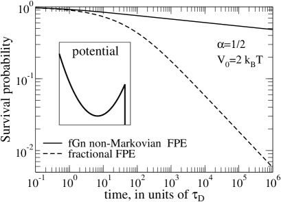
Figure 1: Comparison between the escape dynamics described by the fractional Fokker-Planck equation and the overdamped, non-Markovian GLE-dynamics in (1)-(5) in a parabolic cusp potential, depicted with the inset.

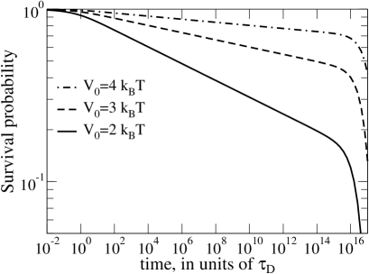
Figure 2: Survival probability for a modified fGn-GLE model using a regularization. An exponential relaxation tail emerges for $t>\omega_{c}^{-1}$. The chosen parameters are: $\tau_{D}\sim{\rm 1\;ps}$, $\omega_{c}\sim{\rm 1\;hour^{-1}}$ and $\alpha=1/2$.

Fig. 1 depicts a comparison between two escape dynamics for $\alpha=1/2$ Xie2 , where $\theta(t)=\exp(t/\tau_{D}){\rm erfc}(\sqrt{t/\tau_{D}})$, and for $\beta V_{0}=2$. The FFP-escape dynamics overall proceeds faster. The initial kinetic stages are identical. A detection of a power-law escape that is exponentially sensitive to temperature would corroborate the GLE based approach; while a temperature-independent power law decay would favor the FFP-approach.

Role of memory cut-off. Both considered theoretical models contain a physical drawback: Random forces obeying a true $1/\omega^{1-\alpha}$ feature in the power spectrum are not physical; i.e. a low-frequency regularization must always emerge on physical grounds, (implying that $S(\omega=0)$ is finite) Weissman . To account for this physical requirement we introduce an exponential cutoff $\exp(-\omega_{c}t)$ with a small frequency $\omega_{c}$ for the memory kernel (5), yielding $S(\omega=0)=2k_{B}T\eta_{\alpha}/\omega_{c}^{1-\alpha}$. The corresponding relaxation function $\theta(t)$ now exhibits an exponential decay $\theta(t)\propto\exp(-\omega_{c}t)$, for $t\geq 1/\omega_{c}$. The memory kernel $\eta(t)$ becomes integrable so that the MFPT $\langle\tau\rangle$ exists. As a consequence, a non-Markovian rate description now becomes valid HTB90 . In practice, however, a feasible rate description fails whenever the main part of the escape dynamics occurs within a distinct non-exponential, power law regime which extends over many temporal decades. This feature is elucidated with Fig. 2. A valid rate description, although with an extremely small rate is restored by either lowering the temperature, or likewise, by increasing the barrier height. The top curve (highest barrier case) in Fig. 2, depicts this trend. Our results corroborate also with the numerical simulations of bistable dynamics Min , where a numerical cut-off is intrinsically present. Using a memory cut-off within the CTRW description for the FFP in Eq. (7) does result as well in an asymptotically finite rate. The intermediate power law will exhibit, however, also no distinct temperature dependence, being again in a clear contrast with the subdiffusive GLE description.

In conclusion, we put forward an analytical treatment of the survival probability for the non-Markovian escape from a cusp-shaped well when anomalous subdiffusion is acting. Then, the MFPT diverges which in turn invalidates a rate description. The sensible physical requirement of a low-frequency regularization enables one to restore a rate theory description that is valid for sufficiently high barriers, or very low temperatures. The single-molecular enzyme kinetics Yang ; Xie2 might present a suitable candidate to validate experimentally the intriguing crossover between an exponential and a power law kinetic regime which crucially depends on temperature.

This work was supported by the German Excellence Initiative via the Nanosystems Initiative Munich (NIM).

References

- (1) H. Scher, E.W. Montroll, Phys. Rev. E 12, 2455 (1975); M. Shlesinger, J. Stat. Phys. 10, 421 (1974).
- (2) R. H. Austin, K. W. Beeson, L. Eisenstein, H. Frauenfelder, and I.C. Gunsalus, Biochemistry 14, 5355 (1975).
- (3) R. Metzler, J. Klafter, Phys. Rep. 339, 1 (2000).
- (4) I.M. Sokolov, J. Klafter, A. Blumen, Phys. Today 55 (11), 48 (2002); J. Klafter, I.M. Sokolov, Physics World, August, 29 (2005).
- (5) J. Tang and R.A. Marcus, Phys. Rev. Lett. 95, 107401 (2005).
- (6) H. Yang et al., Science 302, 262 (2003); H. Yang and X. S. Xie, J. Chem. Phys. 117, 10965 (2002).
- (7) S.C. Kou, X.S. Xie, Phys. Rev. Lett. 93, 180603 (2004); W. Min, G. Luo, B. J. Cherayil, S. C. Kou, and X. S. Xie, Phys. Rev. Lett. 94, 198302 (2005).
- (8) F. Amblard, A. C. Maggs, B. Yurke, A. N. Pargellis, and S. Leibler, Phys. Rev. Lett. 77 4470 (1996); I.Y. Wong et al., Phys. Rev. Lett. 92, 178101 (2004).
- (9) A. Caspi, R. Granek, and M. Elbaum, Phys. Rev. E 66, 011916 (2002).
- (10) M. J. Saxton, Biophys. J. 81, 2226 (2001); I. M. Tolić-Nørrelykke, E.-L. Munteanu, G. Thon, L. Oddershede, and K. Berg-Sørensen, Phys. Rev. Lett. 93, 078102 (2004); M. Weiss, M. Elsner, F. Kartberg, and T. Nilsson, Biophys. J. 87, 3518 (2004); I. Golding and E.C. Cox, Phys. Rev. Lett. 96, 098102 (2006).
- (11) I. Goychuk and P. Hänggi, Phys. Rev. E 70, 051915 (2004).
- (12) G.H. Weiss, Aspects and Applications of the Random Walk (North-Holland, Amsterdam, 1994).
- (13) R. Metzler, E. Barkai, J. Klafter, Phys. Rev. Lett. 82, 3563 (1999); R. Metzler, E. Barkai, J. Klafter, Europhys. Lett. 46, 431 (1999); E. Barkai, Phys. Rev. E 63, 46118 (2001).
- (14) I. Goychuk, E. Heinsalu, M. Patriarca, G. Schmid, and P. Hänggi, Phys. Rev. E 73, 020101(R) (2006).
- (15) P. Hänggi, P. Talkner, M. Borkovec, Rev. Mod. Phys. 62, 251 (1990).
- (16) J. D. Bao, Y. Z. Zhuo, F. A. Oliveira, and P. Hänggi, Phys. Rev. E 74, 061111 (2006).
- (17) B. B. Mandelbrot and J. W. van Ness, SIAM Rev. 10, 422 (1968).
- (18) K.G. Wang and M. Tokuyama, Physica A 265, 341 (1999); R. Kupferman, J. Stat. Phys. 114, 291 (2004).
- (19) A. R. Bizzarri and S. Cannistraro, J. Phys. Chem. B 106, 6617 (2002); G. R. Kneller and K. Hinsen, J. Chem. Phys. 121, 10278 (2004); G. Luo, I. Andricioaei, X. S. Xie, and M. Karplus, J. Phys. Chem. B 110, 9363 (2006).
- (20) S. Chaudhury and B. J. Cherayil, J. Chem. Phys. 125, 024904 (2006); ibid. 125, 114166 (2006).
- (21) S. A. Adelman, J. Chem. Phys. 64, 124 (1976).
- (22) P. Hänggi and H. Thomas, Z. Physik B 26, 85 (1977); P. Hänggi, H. Thomas, H. Grabert, and P. Talkner, J. Stat. Phys. 18, 155 (1978); P. Hänggi, Z. Physik B 31, 407 (1978).
- (23) P. Hänggi and F. Mojtabai, Phys. Rev. A 26, 1168 (1982).
- (24) J. T. Hynes, J. Phys. Chem. 90, 3701 (1986).
- (25) M. B. Weissman, Rev. Mod. Phys. 60, 537 (1988).
- (26) R. Gorenflo, F. Mainardi, in: Fractals and Fractional Calculus in Continuum Mechanics, edited by A. Carpinteri, F. Mainardi (Springer, Wien, 1997), pp. 223-276.
- (27) K. Weron, M. Kotulski, Physica A 232, 180 (1996); R. Hilfer, J. Non-Cryst. Sol. 305, 122 (2002).
- (28) A. A. Stanislavsky, Phys. Rev. E 67, 021111 (2003).
- (29) Even if the exact Green function is known Hynes , the resulting eigenfunctions expansion is required nevertheless for the escape problem.
- (30) Here, a non-natural boundary condition must be used. Our case of a cusp-shaped parabolic well with its a sudden drop to mimics an absorbing line, . Any initial distribution relaxes on the time scale to a quasi-equilibrium Gaussian density with a width around , and gradually decays due to escape.
- (31) W. Min and X. S. Xie, Phys. Rev. E 73, 010902(R) (2006).