Very large stochastic resonance gains in finite sets of interacting identical subsystems driven by subthreshold rectangular pulses

Abstract

We study the phenomenon of nonlinear stochastic resonance (SR) in a complex noisy system formed by a finite number of interacting subunits driven by rectangular pulsed time periodic forces. We find that very large SR gains are obtained for subthreshold driving forces with frequencies much larger than the values observed in simpler one-dimensional systems. These effects are explained using simple considerations.

The phenomenon of stochastic resonance (SR) seems to be important in a wide variety of contexts in physics, chemistry, and the life sciences Gammaitoni et al. (1998). A lot of work has been devoted to the study of SR both in simple Hänggi (2002) and complex systems Jung and Mayer-Kress (1995), such as in ion channel assemblies Schmid et al. (2001) or globally coupled networks of noisy neural elements Zhou et al. (2003), to name a few examples. In this work, we consider a complex system formed by a finite number of $N$ coupled noisy bistable subsystems, the attention to finite sets being inspired by the fact that certain processes in neuroscience seem to involve a rather small number of subsystems Abarbanel et al. (1996).

The signal-to-noise ratio (SNR) and the SR gain are two common quantifiers used to characterize the SR response of noisy systems driven by time-periodic forces. We will study SR effects on a collective variable of finite sets of interacting subunits driven by periodic rectangular pulses. Our results show a tremendous enhancement of SR effects in this collective variable with respect to those observed in single unit systems.

Let us consider a set of $N$ interacting subsystems, each one of them characterized by a single degree of freedom $x_{i}$ ($i=1,\ldots,N$), whose dynamics is governed by the Langevin equations Kometani and Shimizu (1975); Desai and Zwanzig (1978); Casado et al. (2006)

$$\dot{x}_{i}=x_{i}-x_{i}^{3}+\frac{\theta}{N}\sum_{j=1}^{N}(x_{j}-x_{i})+\xi_{i}(t)+F(t),$$ (1)

where $\xi_{i}(t)$ are Gaussian white noises with zero average and $\langle\xi_{i}(t)\xi_{j}(s)\rangle=2D\delta_{ij}\delta(t-s)$, $\theta$ is the parameter defining the strength of the interaction between subsystems, and $F(t)$ is an external driving force of period $T$. In this work, we will restrict ourselves to forces of the type Casado-Pascual et al. (2004)

$$F(t)=\left\{\begin{array}[]{lll}A&;&0\leq t<t_{c},\\ 0&;&t_{c}\leq t<T/2,\\ -A&;&T/2\leq t<T/2+t_{c},\\ 0&;&T/2+t_{c}\leq t<T.\end{array}\right.$$ (2)

The parameter $r=2t_{c}/T$, usually called duty cycle, measures the fraction of a period during which this driving force has a nonvanishing value. In addition, we will only consider subthreshold amplitudes $A$, so that the driving force (2) cannot induce sustained oscillations between dynamical attractors in the absence of noise. The model described by Eq. (1) (without the external periodic driving) was used years ago by Kometani and Shimizu Kometani and Shimizu (1975) as an empirical model to describe muscle contraction. Later on, Desai and Zwanzig Desai and Zwanzig (1978) gave a more detailed statistical mechanical description in the asymptotic $N\rightarrow\infty$ limit and used it to model order-disorder transitions. The addition of an external driving can, in principle, be used to describe the phenomenology of a forced contracting muscle.

We focus on the collective variable $S(t)$ defined as

$$S(t)=\frac{1}{N}\sum_{i=1}^{N}x_{i}(t),$$ (3)

which has previously been used Casado et al. (2006) in the global analysis of coupled bistable systems. It might be considered as the total output process of a parallel array of N indentical interacting subunits, subject to independent noise sources, $\xi_{i}(t)$ and the same external forcing $F(t)$. Its signal-to-noise ratio ($R_{\mathrm{out}}$) is defined in the usual way as,

$$R_{\mathrm{out}}=\frac{Q_{u}}{Q_{l}},$$ (4)

with

$$Q_{u} = \frac{2}{T}\int_{0}^{T}d\tau\,C_{\mathrm{coh}}(\tau)\cos(\Omega\tau)$$ (5)

$$Q_{l} = \frac{2}{\pi}\int_{0}^{\infty}d\tau\,C_{\mathrm{incoh}}(\tau)\cos(\Omega\tau).$$ (6)

where $\Omega=2\pi/T$, $C_{\mathrm{coh}}(\tau)=\frac{1}{T}\int_{0}^{T}dt\langle S(t+\tau)\rangle_{\infty}\langle S(t)\rangle_{\infty}$ and $C_{\mathrm{incoh}}(\tau)=C(\tau)-C_{\mathrm{coh}}(\tau)$ with $C(\tau)=\frac{1}{T}\int_{0}^{T}dt\langle S(t+\tau)S(t)\rangle_{\infty}$.

For a set of $N$ coupled linear oscillators driven by the external driving force $F(t)$ and subject to the noise terms $\xi_{i}(t)$ as in Eq. (1), the SNR of the corresponding collective process, $R_{\mathrm{out}}^{(L)}$, coincides with that of the random process formed by the arithmetic mean of the individual noise terms $\xi_{i}(t)$ plus the deterministic driving force $F(t)$, namely, $F(t)+\xi(t)$ with $\xi(t)=N^{-1}\sum_{i=1}^{N}\xi_{i}(t)$. The process $\xi(t)$ is a Gaussian white noise of effective strength $D/N$. Then, it is easy to prove that

$$R_{\mathrm{out}}^{(L)}=\frac{2A^{2}N[1-\cos(\pi r)]}{\pi D}.$$ (7)

Thus, for our nonlinear case, it seems convenient to analyze the SR gain, $G$, defined as Casado et al. (2006)

$$G=\frac{R_{\mathrm{out}}}{R_{\mathrm{out}}^{(L)}},$$ (8)

which compares the SNR of a non-linear system with that of a linear system subject to the same stochastic and deterministic forces.

We have carried out extensive simulations of the Langevin equations (1) with the external driving (2). In all cases reported here the coupling strength is fixed to $\theta=0.5$ and the subthreshold driving amplitude to $A=0.3$. There is nothing special about this particular $\theta$ value. The qualitative results would be the same for any other value of $\theta\neq 0$.

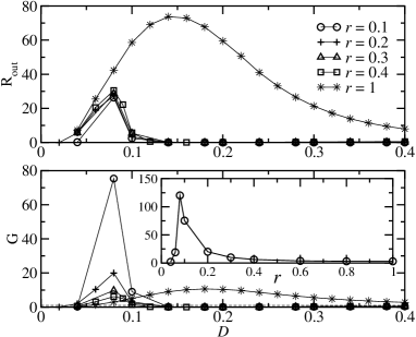
Figure 1: Dependence of the signal-to-noise ratio $R_{\mathrm{out}}$ and the SR gain $G$ for a set of $N=10$ identical subsystems and an external driving of frequency $\Omega=0.01$ for several values of the duty cycle $r$: 0.1 (open circles), 0.2 (crosses), 0.3 (triangles), 0.4 (squares), and 1 (stars). Inset shows the SR gain as a function of $r$ for a fixed noise strength $D=0.08$. The lines have been drawn as a guide to the eye.

In Fig. 1 we show the collective signal-to-noise ratio and SR gain as a function of the noise strength $D$ for a set of $N=10$ identical subsystems, a driving fundamental frequency $\Omega=0.01$ and several values of the duty cycle $r$. It can be seen that, while the SNR curves are nearly identical for $r\leq 0.4$, the SR gain increases drastically, reaching a very large value for $r=0.1$. This dramatic increase is easily understood by taking into account the observed almost constant behavior of $R_{\mathrm{out}}$ and the fact that $R_{\mathrm{out}}^{(L)}$, Eq. (7), decreases monotonically with $r$. However, for sufficiently small $r$, $R_{\mathrm{out}}$ must decrease faster than $R_{\mathrm{out}}^{(L)}$, because the interval $t_{c}$ becomes smaller than the time it takes for the system to react to a constant force of amplitude $A$, and thus, the driving produces almost no effect in the system. This behavior is shown in the inset of Fig. 1, where it can be seen that the SR gain decreases for $r\leq 0.08$. Also, as seen in Fig. 1, when $r=1$ (rectangular driving signal), $G$ reaches a peak at a noise value $D\approx 0.2$. Even though $R_{\mathrm{out}}^{(L)}$ is as large as it can be, the huge increase of $R_{\mathrm{out}}$ is enough to overcome the increase in $R_{\mathrm{out}}^{(L)}$, yielding a substantial value for the SR gain.

The very large gain values in Fig. 1 for pulses with short duty cycles are observed only for a small range of noise strengths around $D\approx 0.08$. In Fig. 2 we present the behavior of $Q_{l}$ and $Q_{u}$ with $D$. Notice that around $D\approx 0.08$ there is a strong reduction of two orders of magnitude in the level of fluctuations of the collective variable as measured by $Q_{l}$. Therefore, the large SR effects quantified by the SNR and the SR gains are essentially due to the very large reduction of the fluctuation spectrum of the output signal at the fundamental driving frequency for a range of noise values.

We have also analyzed the SNR and the SR gain for different values of $\Omega$. Our results for $R_{\mathrm{out}}$ and $G$ as a function of $D$ are depicted in Fig. 3 for a set of $N=10$ interacting identical subunits driven by rectangular pulses with duty cycle $r=0.1$ and several values of the fundamental driving frequency $\Omega$: 0.015 (open circles), 0.02 (crosses), 0.03 (triangles), and 0.04 (squares). As we increase the driving frequency $\Omega$, the SR gain is gradually reduced. For a sufficiently large driving frequency (pulses of very short duration), gains larger than unity are not observed for any value of the noise strength.

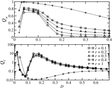
Figure 2: Dependence of the denominator and the numerator of the collective signal-to-noise ratio for the same parameter values as in Fig 1. The lines have been drawn as a guide to the eye.

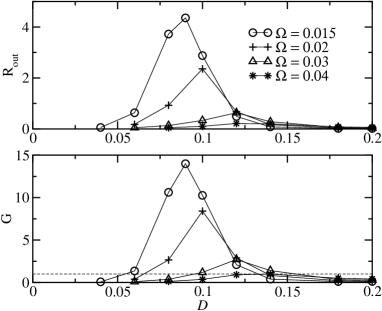
Figure 3: Dependence of the signal-to-noise ratio and the SR gain for a set of $N=10$ identical subsystems and duty cycle $r=0.1$ for several values of the driving frequency $\Omega$: 0.015 (open circles), 0.02 (crosses), 0.03 (triangles), and 0.04 (squares). Solid lines have been drawn as a guide to the eye. The horizontal dashed line marks the unity for the SR gain.

As mentioned above, the large SNR values observed in Fig. 1 are related to the existence of a sharp minimum of $Q_{l}$ at a certain noise value. As observed in Fig. 2, this value is $D\approx 0.08$ for a driving signal with short duty cycle, amplitude $A=0.3$ and fundamental frequency $\Omega=0.01$. For other amplitude and frequency, the location of the minimum will change, although the mechanisms leading to the existence of this minimum will be qualitatively the same.

To understand the $Q_{l}$ dependence on $D$, it is important to analyze in detail the dynamics imposed by the external driving force in Eq. (2). For the $D$ and $\theta$ values of interest to the present discussion, simulations show that when the driver is absent, the collective variable $S(t)$ performs a noise induced random movement between the two symmetric attractors of the dynamics, which we will regard as located at $\pm S_{0}$. During a time interval of duration $t_{c}$, the external force $F(t)=A$ favors the positive attractor. Thus, if $S(t)$ was at the negative attractor at the beginning of the interval, the external forcing will drive it to the positive one in a random time that we will denote by $\Upsilon_{1}$. Certainly, different realizations of the noise will yield different values of $\Upsilon_{1}$. Running simulations with many independent trajectories, we have computed the probability $\mathrm{Prob}(\Upsilon_{1}<\tau)=f(\tau)$ that the variable $S(t)$ has jumped before a time $\tau$ to the attractor favored by a constant driving of amplitude $A$. In Fig. 4 (a) we present $f(\tau)$ for the set of parameters relevant to the discussion: $A=0.3$, $D=0.08$, and $N=10$ (solid line). It can be seen that for the case $r=0.1$ and $\Omega=0.01$, (thus, $t_{c}\approx 31.4$), a transition between the attractors for $\tau=t_{c}$ is performed with probability almost unity. Then, during the rest of the half-period, an interval of duration $T/2-t_{c}$, the external force is zero and the system is free to jump between the attractors due solely to noise. Let us now denote by $\Upsilon_{2}$ the random time it takes to jump from one attractor to the opposite one when $F(t)=0$. Figure 4 (b) shows the probability $\mathrm{Prob}(\Upsilon_{2}<\tau)=g(\tau)$ that this jump has taken place before a time $\tau$ vs. $\tau$. Since for $r=0.1$ and $\Omega=0.01$ we have $T/2-t_{c}\approx 282.7$, it can be checked in Fig. 4 (b) that almost no transitions take place during this time interval under these conditions. We can carry out the same analysis for the symmetric situation during the second half-period of the driving force. Consequently, $S(t)$ performs a neat trajectory between its attractors with transitions induced systematically every half-period by the external driving when it has a nonvanishing value. As a result, we would expect $C_{\mathrm{incoh}}(0)$, itself an average of the second cumulant of $S(t)$ over a period, to be of the order of the effective noise $D/N$, and $C_{\mathrm{incoh}}(\tau)$ short-lived. This is, in fact, what is observed in Fig. 5 (see inset).

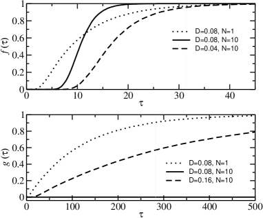
Figure 4: (a) Probability that the collective variable $S(t)$ has jumped before a time $\tau$ to the attractor favored by an external constant driving of amplitude $A=0.3$ starting from the opposite attractor. The solid line corresponds to a system with $D=0.08$ and $N=10$, the dotted line to $D=0.08$ and $N=1$, and the dashed line to $D=0.04$ and $N=10$. (b) Probability that $S(t)$ jumps before a time $\tau$ to the opposite attractor in the absence of driving. The solid line corresponds to a system with $D=0.08$ and $N=10$ (being almost zero for the range of times shown), the dotted line to $D=0.08$ and $N=1$, and the dashed line to $D=0.16$ and $N=10$.

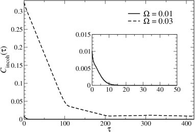
Figure 5: Temporal behavior of the incoherent part of the correlation function of the collective variable for a system of $N=10$ identical subsystems with $D=0.08$ and $r=0.1$. The solid lines correspond to $\Omega=0.01$ and the dashed line to $\Omega=0.03$. The inset is a magnification of the case $\Omega=0.01$ displayed for the sake of clarity.

The curves in Fig. 4(a) indicate that the probability of transitions between the attractors before $t_{c}$ out of the most unstable attractor is smaller for $D=0.04$ than for $D=0.08$. This is to be expected as the probability of transitions out of an attractor goes to zero when $D\to 0$ with subthreshold driving amplitudes. As a result, $C_{\mathrm{incoh}}(0)$ and the decay time of $C_{\mathrm{incoh}}(\tau)$ increase as $D$ gets smaller than $D=0.08$. Consequently, noticing its definition in Eq. (6), $Q_{l}$ has to increase as $D$ is reduced from $D=0.08$.

Fig. 2 shows that for noise values larger than $D\approx 0.08$ the $Q_{l}$ dependence on $D$ for inputs with short duty cycles is rather different from the one observed for a rectangular input ($r=1$). This fact indicates that for short duty cycles and these larger noise values, the time intervals during which $F(t)=0$ are crucial for the system response. By comparing the $g(\tau)$ curves for $D=0.08$ and $D=0.16$ in Fig. 4 (b), we see that the probability of transitions between attractors during the time interval $T/2-t_{c}$ is negligible, whereas there is a non-negligible probability for $D=0.16$. Therefore, the bimodal character of the probability distribution for $S(t)$ is enhanced as $D$ increases from $D\approx 0.08$ to $D\approx 0.16$ and one can then conclude that $C_{\mathrm{incoh}}(0)$ and the decay time of $C_{\mathrm{incoh}}(\tau)$ increase as $D$ increases. Consequently, for short duty cycles, $Q_{l}$ also increases as $D$ increases within the interval $D\approx 0.08$ to $D\approx 0.16$. On the other hand, for $r=1$ and this same range of noise values, the situation is different because the driving signal never vanishes. Then, transitions out of the most unstable attractor happen more frequently as noise increases [$f(\tau)$ saturates at $1$ earlier], and this leads to a decrease of both $C_{\mathrm{incoh}}(0)$ and the decay time of $C_{\mathrm{incoh}}(\tau)$ as $D$ increases, with the corresponding decrease in $Q_{l}$.

Similarly, raising the driving fundamental frequency has a drastic effect on the behavior of $C_{\mathrm{incoh}}(\tau)$ with respect to its optimal behavior discussed above for $D=0.08$ and $r=0.1$, as depicted in Fig. 5 for two frequency values: $\Omega=0.01$ and $\Omega=0.03$ . The picture that emerges for $\Omega=0.03$, differs considerably from that observed for $\Omega=0.01$. For the higher frequency case, with $t_{c}\approx 10.4$, the value of the solid line at $\tau=10.4$ in Fig. 4 (a) indicates that, for a considerable number of trajectories, the driving force is not able to induce a transition during the time interval $t_{c}$. Consequently, the second cumulant of $S(t)$ becomes of the order of the distance between the attractors. On the other hand, for the lower frequency, transitions occur for the corresponding $\tau=t_{c}\approx 31.4$ with almost total certainty. This leads to a $C_{\mathrm{incoh}}(0)$ for $\Omega=0.03$ much larger than for $\Omega=0.01$. Additionally, since still almost no transitions occur at the intervals when the driving is absent, as shown in Fig. 4 (b), nor obviously when the driving favors the initial attractor, any unsuccessful transition is carried on until the next period, and we would expect a long-lived $C_{\mathrm{incoh}}(\tau)$. Namely, noise induced correlations persist during a few driving periods. These observations justify the full behavior observed in Fig. 5.

In conclusion, we have analyzed the enhancement of SR effects in a collective variable characterizing the response of finite sets of interacting noisy subsystems. The cooperative effect of noise and nonlinearity in finite sets of interacting, driven, bistable subunits reflects in a substantial decrease in the noise level of the collective output, $S(t)$, with respect to that observed in the output of a single independent unit. Very large values of the SR gain can be achieved for trains of short rectangular pulses of the type defined by Eq. (2). Even though the results presented here have been obtained with external pulses with very brisk changes of their amplitudes at certain instants of time, similar results can also be observed when the pulse amplitude changes continuously, as long as there are time intervals within a period where the amplitude changes very slowly, followed by short time intervals where the amplitude changes very drastically.

This research was supported by the Dirección General de Enseñanza Superior of Spain (Grant No. FIS2005-02884), the Junta de Andalucia, and the Juan de la Cierva program of the Ministerio de Ciencia y Tecnología (D.C.).

References

- Gammaitoni et al. (1998) L. Gammaitoni, P. Hänggi, P. Jung, and F. Marchesoni, Rev. Mod. Phys. 70, 223 (1998).
- Hänggi (2002) P. Hänggi, ChemPhysChem. 3, 285 (2002).
- Jung and Mayer-Kress (1995) P. Jung and G. Mayer-Kress, Phys. Rev. Lett. 74, 2130 (1995); J. F. Lindner, B. K. Meadows, W. L. Ditto, M. E. Inchiosa, and A. R. Bulsara, ibid. 75, 3 (1995); A. Pikovsky, A. Zaikin, and M. A. de la Casa, ibid. 88, 050601 (2002).
- Schmid et al. (2001) G. Schmid, I. Goychuk, and P. Hänggi, Europhys. Lett. 56, 22 (2001).
- Zhou et al. (2003) C. Zhou, J. Kürths, and B. Hu, Phys. Rev. E 67, 030101(R) (2003); J. A. Acebrón, A. R. Bulsara, and W. J. Rappel, ibid. 69, 026202 (2004).
- Abarbanel et al. (1996) H. Abarbanel et al., Phys. Usp. 39, 337 (1996).
- Kometani and Shimizu (1975) K. Kometani and H. Shimizu, J. Stat. Phys. 13, 473 (1975).
- Desai and Zwanzig (1978) R. Desai and R. Zwanzig, J. Stat. Phys. 19, 1 (1978).
- Casado et al. (2006) J. M. Casado, J. Gómez-Ordóñez, and M. Morillo, Phys. Rev. E 73, 011109 (2006); J. Casado-Pascual, J. Gómez-Ordóñez, and M. Morillo, Chaos, 15, 026115 (2005)
- Casado-Pascual et al. (2004) J. Casado-Pascual, J. Gómez-Ordóñez, and M. Morillo, Phys. Rev. E 69, 067101 (2004).