Exact Activation Energy of Magnetic Single Domain Particles

Abstract

I present the exact analytical expression for the activation energy as a function of externally applied magnetic fields for a single–domain magnetic particle with uniaxial anisotropy (Stoner–Wohlfahrt model), and investigate the scaling behavior of the activation energy close to the switching boundary. PACS numbers: 75.75.+a, 75.45.+j, 75.10.-b

I Introduction

A lot of effort has been spent over the last few years to understand the magnetization reversal of small magnetic particles Lederman94 ; Kent94 ; Wernsdorfer95 ; Koch98 ; Bonet99 ; Wernsdorfer00 ; Schumacher03 . At sufficiently low temperatures, macroscopic quantum tunneling has been observed Coppinger95 ; Friedmann96 ; Wernsdorfer97 ; Bokacheva00 , while for higher temperatures thermally activated behavior may switch the magnetization of the particle Koch00 . For the anlaysis of the experiments one needs to know the activation energy. Moreover, with the advancing developement of integrated magnetoresistive memory devices (MRAM) the dependence of the energy barrier on the magnetic field has become of crucial technological importance as well. In a typical MRAM array, magnetic memory cells are written by a coincident field technique, where both a selected bitline (BL) and a selected wordline (WL) create magnetic fields, the sum of which are strong enough to switch the memory cell, whereas the fields from either BL or WL alone are not sufficient to switch the cell. Nevertheless, these fields do destabilize the non–selected cells to some extent, i.e. they reduce the energy barrier against thermally activated switching. Also, even for the selected cells the switching at finite temperatures happens before the actual zero temperature boundary of stability is reached, again due to thermal activation during the finite duration of a write pulse Koch00 ; Braun93 . To estimate the life time of the information in the memory, one needs to know the dependence of the energy barrier on the applied fields as precisely as possible, as the energy barrier enters the switching rate exponentially.

In the study of the switching behavior of small size magnetic particles, the Stoner Wohlfarth model plays a central role Stoner48 . It describes a single domain particle with uni–axial anisotropy in an external magnetic field. The single domain approximation greatly simplifies the analysis, and becomes a good approximation if the size of the particle becomes comparable to or smaller than the exchange length, which in memory elements etched out of a thin magnetic film is typically of the order of 100nm. The activation energy in the Stoner Wohlfarth model can be calculated trivially if the external field is aligned either parallel to the preferred axis or perpendicular to it. However, so far no analytical solution has been known for the general case of the external field pointing in an arbitrary direction Wernsdorfer03 . Given the crucial importance of the field dependence of the activation energy, an exact analytical solution will be provided in the present paper.

II The Stoner Wohlfarth Model

The energy of a uniformly magnetized particle with uniaxial symmetry, characterized by the anistropy energy density $K$ and saturation magnetization $M_{s}$ depends on its magnetization via the angle $\vartheta$ between the magnetization and the preferred axis,

$$E(\vartheta)=KV\sin^{2}\vartheta-VM_{s}H_{x}\cos\vartheta-VM_{s}H_{y}\sin\vartheta\,,$$ (1)

where $H_{x}$ and $H_{y}$ are the magnetic field components parallel and perpendicular to the preferred axis in a plane containing the magnetization and the preferred axis, respectively, and $V$ denotes the volume of the sample Stoner48 . In the following dimensionless variables will be used by writing the energy in terms of $2KV$, $e(\vartheta)=E(\vartheta)/(2KV)$, and the magnetic field components in terms of the switching field $H_{c}=2K/M_{s}$ as $h_{x}=H_{x}/H_{c}$, $h_{y}=H_{y}/H_{c}$, such that

$$e(\vartheta)=\frac{1}{2}\sin^{2}\vartheta-h_{x}\cos\vartheta-h_{y}\sin\vartheta\,.$$ (2)

For vanishing magnetic fields, this model has a bistable ground state, whereas for very large fields ($h_{x}\gg 1$ or $h_{y}\gg 1$) the first term can be neglected, and there is only one minimum in the interval $-\pi\leq\vartheta<\pi$, such that the magnetization tends to align parallel to the applied field. Thus, for increasing field, one of the original minima has to disappear, and the fields where this happens mark the boundary of bistability. These fields are easily obtained by setting both the first and second derivative of (2) to zero and eliminating $\vartheta$, whereupon the famous Stoner-Wohlfahrt astroid $h_{x}=\cos^{3}\vartheta$, $h_{y}=\sin^{3}\vartheta$ is obtained Stoner48 .

III Activation Energy

The activation energy can in principle be calculated in a straight forward manner by finding the two minima and the two maxima of the energy in the bistability range, determining the metastable of the two minima and the energy barrier to the smaller of the two maxima barrier . In the case of $h_{x}=0$ or $h_{y}=0$ this is straight forward: For $h_{y}=0$,

$$\frac{\partial e}{\partial\vartheta}=\cos\vartheta\sin\vartheta+h_{x}\sin\vartheta-h_{y}\cos\vartheta=0$$ (3)

leads to $\vartheta=0$, $\vartheta=\pi$, or $\cos\vartheta=-h_{x}$. The solution $\vartheta=0$ is metastable for $-1\leq h_{x}\leq 0$, stable for $h_{x}>0$, and unstable for $h_{x}<-1$. Correspondingly, $\vartheta=\pi$ is metastable for $0\leq h_{x}<1$, stable for $h_{x}<0$, and unstable for $h_{x}>1$. The solution $cos\vartheta=-h_{x}$ leads to two maxima which become complex for $|h_{x}|>1$. Thus, the energy barrier for switching from $\vartheta=\pi$ to $\vartheta=0$ is given by $E_{A}=e(\arccos(-h_{x}))-e(\pi)=(1-h_{x})^{2}/2$. Similarly, for $h_{x}=0$ one finds the energy barrier $E_{A}=(1-h_{y})^{2}/2$. Therefore, if one of the two field components vanishes, the activation energy depends quadratically on the distance from the stability boundary.

In the general case, where neither $h_{x}$ nor $h_{y}$ vanish, one may substitute $\sin\vartheta=u$, $\cos\vartheta=\pm\sqrt{1-u^{2}}$ into (3). Squaring the equation leads to

$$-u^{4}+2u^{3}h_{y}+u^{2}(1-h_{x}^{2}-h_{y}^{2})-2uh_{y}+h_{y}^{2}=0\,.$$ (4)

In order to calculate the energy barrier, one needs to find the roots of this 4th order polynomial, which makes the analysis much more cumbersome than for $h_{x}h_{y}=0$. Still, the roots of a 4th order polynomial can be obtained analytically. The solutions $\vartheta_{i}$ are conveniently written in terms of the functions

$$f_{1} = h_{x}^{2}+h_{y}^{2}-1\,,$$ (5)

$$f_{2} = 108h_{x}^{2}h_{y}^{2}+2f_{1}^{3}\,,$$ (6)

$$f_{3} = f_{2}+\sqrt{f_{2}^{2}-4f_{1}^{6}}\,,$$ (7)

$$f_{4} = \sqrt{1+\frac{f_{1}}{3}+\frac{2^{1/3}}{3}\frac{f_{1}^{2}}{f_{3}^{1/3}}+\frac{1}{3}\frac{f_{3}^{1/3}}{2^{1/3}}-h_{y}^{2}}\,.$$ (8)

Eq.(4) has four solutions for $u$, but the ambiguity in the sign of $\cos\vartheta$ in terms of $u$ leads at this point to eight solutions for $\vartheta$. They differ by three signs $\mu,\nu,\sigma$ in various places, and are given by

$$\vartheta_{i} = \sigma\arccos\Bigg{[}-\frac{h_{x}}{2}+\frac{\mu}{2}f_{4}+\frac{\nu}{2}\sqrt{1-\frac{f_{1}}{3}-\frac{2^{1/3}f_{1}^{2}}{3f_{3}^{1/3}}-\frac{1}{3}\frac{f_{3}^{1/3}}{2^{1/3}}+h_{x}^{2}-h_{y}^{2}+\frac{2\mu}{f_{4}}(2h_{x}+f_{1}h_{x}-h_{x}^{3})}\Bigg{]}\,.$$ (9)

The signs will be chosen according to the binary decomposition $(\mu,\nu,\sigma)=(-,-,-)$ for $\vartheta_{1}$, $(-,-,+)$ for $\vartheta_{2}$, $(-,+,-)$ for $\vartheta_{3}$, $\ldots$, $(+,+,+)$ for $\vartheta_{8}$. None of these solutions solves (3) for all $h_{x},h_{y}$. Rather, each of them solves the equation only in two quadrants. However, it is possible to construct four uniform solutions out of the eight partially valid ones, which are continuous (after the identification of $\pi$ with $-\pi$) and solve (3) for all values of $h_{x},h_{y}$. The four uniform solutions are

$$\tilde{\vartheta}_{1} = \theta(h_{y})\vartheta_{2}+\theta(-h_{y})\vartheta_{1}\,,$$ (10)

$$\tilde{\vartheta}_{2} = \theta(h_{x}h_{y})\vartheta_{5}+\theta(-h_{x}hy)\vartheta_{3}\,,$$ (11)

$$\tilde{\vartheta}_{3} = \theta(h_{x}h_{y})\vartheta_{4}+\theta(-h_{x}hy)\vartheta_{6}\,,$$ (12)

$$\tilde{\vartheta}_{4} = \theta(h_{y})\vartheta_{8}+\theta(-h_{y})\vartheta_{7}\,,$$ (13)

where $\theta(x)=1$ for $x>0$ and zero elsewhere denotes the Heaviside function. Calculating the second derivative one finds that the first uniform solution is a minimum for $h_{x}<0$. It disappears as real solution for $h_{x}>0$ outside the astroid. Thus, this is the metastable state for $h_{x}>0$. On the other hand, $\tilde{\vartheta}_{4}$ remains a minimum even outside the astroid for $h_{x}>0$, but disappears as real solution outside the astroid for $h_{x}<0$. The uniform solutions $\tilde{\vartheta}_{2}$ and $\tilde{\vartheta}_{3}$ are both maxima inside the astroid, and become complex outside one half of the astroid (for $h_{y}<0$ and $h_{y}>0$, respectively ??). One easily convinces oneself that for $h_{y}\geq 0$, $\tilde{\vartheta}_{3}$ is the relevant maximum ($e(\tilde{\vartheta}_{3})\leq e(\tilde{\vartheta}_{2})$), whereas for $h_{y}<0$, escape over the maximum at $\tilde{\vartheta}_{2}$ is dominant ($e(\tilde{\vartheta}_{3})>e(\tilde{\vartheta}_{2})$). The activation energy out of the metastable state is therefore given by

$$E_{A} = e(\tilde{\vartheta}_{3})-e(\tilde{\vartheta}_{1})\mbox{ for }h_{y}\geq 0\,,$$ (15)

$$E_{A} = e(\tilde{\vartheta}_{2})-e(\tilde{\vartheta}_{1})\mbox{ for }h_{y}<0\,,$$ (16)

Fig.1 shows a plot of the activation energy as function of $h_{x}$ and $h_{y}$.

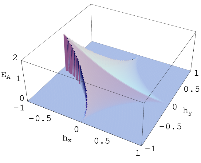
Figure 1: Activation energy as function of $h_{x}$ and $h_{y}$, out of the state stable for $h_{x}<0$. Outside the astroid there is only one stable and no metastable state, and the activation energy is therefore undefined.

For $h_{y}=0$ both maxima lead to the same activation energy, and $E_{A}$ is an even function of $h_{y}$, as it should be. In the following the attention will therefore focus solely on the case $h_{y}\geq 0$, and to the case where the initial state $\vartheta=\pi$ is metastable, $h_{x}>0$, i.e. the first quadrant. In principle, the particle might be excited also out of the stable state and end up (for a finite time) in the metastable state, but this process is of much less importance, as the activation energy is much larger and it enters exponentially in the thermal switching rate.

IV Scaling

The scaling of the activation energy as function of the distance $1-h$ from the astroid boundary is of particular interest. Here, $h$ is defined by $h_{x}=h\cos^{3}\xi$, $h_{y}=h\sin^{3}\xi$ such that $h=1$ always corresponds to the astroid boundary. It has been shown before Wernsdorfer96 that the scaling must be of the form

$$E_{A} = c_{3/2}(\xi)(1-h)^{3/2}+c_{2}(\xi)(1-h)^{2}+c_{5/2}(\xi)(1-h)^{5/2}+\ldots\,.$$ (17)

All coefficients besides $c_{2}(\xi)$ vanish for $\xi=0$, and but it has been shown numerically Wernsdorfer96 and theoretically Victora89 that already for small values of $\xi$ the coefficient $c_{3/2}$ dominates the scaling. This is confirmed and made more precise by using the exact solution. Fig. 2 shows $\ln E_{A}$ as function of $\ln(1-h)$. The plot reveals power law behavior to a good approximation even rather far away from the astroid boundary, $E_{A}\propto(1-h)^{a}$ with an exponent $a=2$ for $\xi=0$, and an exponent close to $3/2$ for larger values of $\xi$.

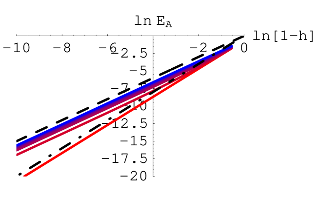
Figure 2: Scaling of the activation energy $E_{A}$ as function of the relative distance $h$ from the astroid boundary ($h_{x}=h\cos^{3}\xi$, $h_{y}=h\sin^{3}\xi$). The curves show decreasing slopes for values of $x=\xi/\pi=0$ (red), $1/24$, (pink) $2/24,\ldots 1/4$ (blue). The dashed line corresponds to a power law with exponent 3/2, the dot–dashed line to an exonent 2.

According to the numerical evaluation of (15) the exponent is symmetric with respect to $\xi=\pi/4$. The exact value of the exponent depends on the fitting range and on whether a quadratic term is included in the fit of $\ln E_{A}$ as function of $\ln(1-h)$. Fig. 3 shows the fitted exponent $a$ as a function of $x=\xi/\pi$ for three different fitting ranges, from $h=0.932$ to $h=0.99999853$, assuming a pure power law, $\ln E_{A}=a\ln(1-h)$. The observed dependence of the exponent on $x$ is very similar to what was previously calculated numerically Wernsdorfer96 . In particular, the exponent appears to become even slightly smaller than $3/2$ for values of $\xi$ close to $\pi/4$.

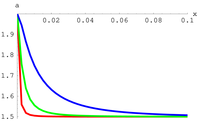
Figure 3: Scaling exponent $a$ extracted from a fit of $\ln E_{A}$ to $a\ln(1-h)$, using the exact expression for $E_{A}$, eq.(15). The three curves correspond to fitting ranges $h=0.93187079$ to $h=0.996837$ (top curve — blue), $h=0.99538$ to $h=0.999978$ (middle curve — green), and $h=0.9996837$ to $h=0.999998532$ (bottom curve — red). For all calculations of the activation energy, 80 digits precision was used.

However, there is a substantial non–linear part in the scaling behavior, as becomes obvious when fitting to $\ln E_{A}=a\ln(1-h)+b\ln^{2}(1-h)$. The extracted linear part is plotted in Fig.4. For small values of $\xi$, the exponent can now be substantially larger than $2$.

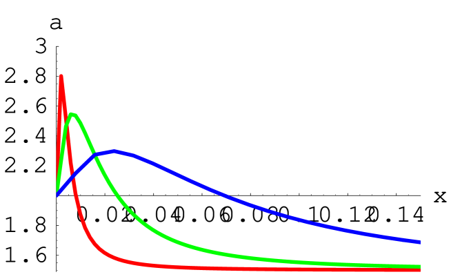
Figure 4: Scaling exponent $a$ extracted from a fit of $\ln E_{A}$ to $a\ln(1-h)+b\ln^{2}(1-h)$. The three curves correspond to the same fitting ranges used in Fig.3.

V Summary

I have derived the exact analytical expression of the activation energy for single domain switching of small magnetic particles in arbitrary magnetic fields (Stoner–Wohlfarth model). The activation energy scales approximately like a power law as a function of the distance of the switching boundary (astroid) up to distances of order unity, but also contains a substantial non–power law term.

Acknowledgement: I am grateful to Daniel Worledge for a useful discussion.

References

- (1) M. Lederman, S. Schultz, and M. Ozaki, Phys. Rev. Lett. 73, 1986 (1994).
- (2) A.D. Kent, S. von Molnar, S. Gider, and D.D. Awschalom, J. Appl. Phys. 76 6656 (1994).
- (3) W. Wernsdorfer et al., J. Magn. Magn. Mater. 151, 396 (1995).
- (4) R.H. Koch, J.G. Dreak, D.W. Abraham, P.L. Trouilloud, R.A. Altman, Y. Lu, W.J. Gallagher, R.E. Scheuerlein, K.P. Roche, and S.S.P. Parkin, Phys. Rev. Lett., 81, 4512 (1998).
- (5) E. Bonet, W. Wernsdorfer, B. Barbara, A. Benoît, D. Mailly, and A. Thiaville, Phys. Rev. Lett. 83, 4188 (1999).
- (6) W. Wernsdorfer, D. Mailly, A. Benoit, J. Appl. Phys., 87, 5094 (2000).
- (7) H.W. Schumacher, C. Chappert, R.C. Sousa, P.P. Freitas, and J. Miltat, Phys. Prev. Lett. 90, 017204 (2003).
- (8) F. Coppinger, J. Genoe, D.K. Maude, U. Gennser, J.C. Portal, K.E. Singer, P. Ruter,T. Taskin, A.R. Peaker, A.C. Wright, Phys. Rev. Lett, 75, 3513 (1995).
- (9) J.R. Friedmann, M.P. Sarachik, J. Tejada, R. Ziolo, Phys. Rev. Lett. 76, 3830 (1996).
- (10) W. Wernsdorfer, E. Bonet Orozco, K. Hasselbach, A. Benoit, D. Mailly, O. Kubo, H. Nakamo, and S. Barbara, Phys. Rev. Lett. 79, 4014 (1997).
- (11) L. Bokacheva, A.D. Kent, and M.A. Walters, Phys. Rev. Lett. 85, 4803 (2000).
- (12) R.H. Koch, G. Grinstein, Y. Lu, P.L. Trouilloud, W.J. Gallagher, and S.S.P. Parkin, Phys. Rev. Lett. 84, 5415 (2000).
- (13) H.-J. Braun, Phys. Rev. Lett. 71, 3557 (1993).
- (14) E.C. Stoner, E.P. Wolfarth, Phil. Trans. Roy. Soc. A 240, 599 (1948).
- (15) W. Wernsdorfer, private communication.
- (16) Note that in principle there are two energy barriers, corresponding to the two escape paths out of the metastable minimum by clockwise or counterclockwise rotation of the magnetization. In the following the path with the higher activation energy will be neglected and the activation energy will always be defined as the smaller of the two energy barriers.
- (17) W. Wernsdorfer, Ph.D. thesis, Université Joseph Fourier–Grenoble I (1996).
- (18) R.H. Victora, Phys. Rev. Lett. 63, 457 (1989)