Integral Field Spectroscopy of the Extended Emission-Line Region of 4C 37.43

Abstract

We present Gemini integral field spectroscopy and Keck II longslit spectroscopy of the extended emission-line region (EELR) around the quasar 4C 37.43. The velocity structure of the ionized gas is complex and cannot be explained globally by a simple dynamical model. The spectra from the clouds are inconsistent with shock or “shock + precursor” ionization models, but they are consistent with photoionization by the quasar nucleus. The best-fit photoionization model requires a low-metallicity (12+log(O/H) $\lesssim$ 8.7) two-phase medium, consisting of a matter-bounded diffuse component with a unity filling-factor ($N\sim 1$ cm^-3, $T\sim 15000$ K), in which are embedded small, dense clouds ($N\sim 400$ cm^-3, $T\sim 10^{4}$ K). The high-density clouds are transient and can be re-generated through compressing the diffuse medium by low-speed shocks ($V_{S}\lesssim 100$ km s^-1). Our photoionization model gives a total mass for the ionized gas of about $3\times 10^{10}$ M_⊙, and the total kinetic energy implied by this mass and the observed velocity field is $\sim 2\times 10^{58}$ ergs. The fact that luminous EELRs are confined to steep-spectrum radio-loud QSOs, yet show no morphological correspondence to the radio jets, suggests that the driving force producing the 4C 37.43 EELR was a roughly spherical blast wave initiated by the production of the jet. That such a mechanism seems capable of ejecting a mass comparable to that of the total interstellar medium of the Milky Way suggests that “quasar-mode” feedback may indeed be an efficient means of regulating star formation in the early universe.

1. Introduction

A number of low-redshift QSOs show luminous extended emission-line regions (EELRs) that have characteristic dimensions of a few tens of kpc, considerably larger than the typical $\sim 1$ kpc of the classical narrow-line regions (NLRs; see Stockton et al. 2006b for a recent brief review of EELRs). In a few cases, such extended emission may be simply due to QSO photoionization of the in situ interstellar medium (ISM) of the host galaxy or of nearby gas-rich dwarf galaxies, but, for the most luminous examples, such explanations are inadequate. These luminous EELRs typically show complex filamentary structures that bear no close morphological relationships either with the host galaxies or with extended radio structures.

In spite of this general lack of attention on the part of EELRs to the structural parameters of their host galaxies, they quite clearly are not oblivious to the properties of the QSOs themselves. As Boroson & Oke (1984) and Boroson et al. (1985) found, and Stockton & MacKenty (1987) confirmed, luminous EELRs are associated virtually exclusively with steep-spectrum radio-loud QSOs. Stockton & MacKenty (1987) also noted a strong correlation between the strength of the nuclear narrow-line emission and that of the extended emission. This latter correlation may not be particularly surprising. However, the restriction of luminous EELRs to steep-spectrum quasars, together with the general lack of correspondence between the distribution of the ionized gas and the radio structure, presents an intriguing puzzle. To add to the confusion, not all low-redshift, steep-spectrum quasars (even among those that have luminous classical NLRs) show luminous extended emission: the fraction that do is $\sim$1/3 to 1/2 (Stockton & MacKenty, 1987).

Early guesses regarding the origin of the extended gas centered on tidal debris (Stockton & MacKenty, 1987) or cooling flows (Fabian et al., 1987). However, as Crawford et al. (1988) correctly pointed out, ionized gas from a tidal encounter would dissipate on a time scale of $\lesssim 10^{6}$ years unless it were confined gravitationally or by the pressure of a surrounding medium. On the other hand, Stockton et al. (2002) showed, from a detailed photoionization model of the EELR around the $z=0.37$ quasar 4C 37.43, that the pressure of any surrounding hot gas was too low for the gas to cool in less that a Hubble time. This conclusion was supported by the lack of evidence for a general distribution of hot gas around 3 quasars in deep Chandra X-ray imaging (Stockton et al., 2006a). Gravitational confinement of the amount of ionized gas seen in many EELRs would imply unreasonably large masses of neutral or otherwise invisible material in the outskirts of the host galaxy.

Given the short lifetime of unconfined ionized filaments and the unlikelihood of gravitational confinement, along with the other constraints we have mentioned, the most likely scenario for producing an EELR is that of a superwind (Stockton et al., 2002; Fu & Stockton, 2006). In principle, such a superwind could result either from a starburst or from feedback from the quasar (e.g., Di Matteo et al. 2005; Hopkins et al. 2006), with some evidence favoring the latter alternative (Fu & Stockton, 2006). Such an origin would be of considerable interest, since it would mean that we have local examples of a process similar (though almost certainly not identical) to the “quasar-mode” feedback mechanism that may be important in initially establishing the observed correlation between bulge mass and black hole mass during galaxy formation in the early universe. In order to explore this possibility in more detail, we have carried out an extensive re-examination of the EELR of 4C 37.43.

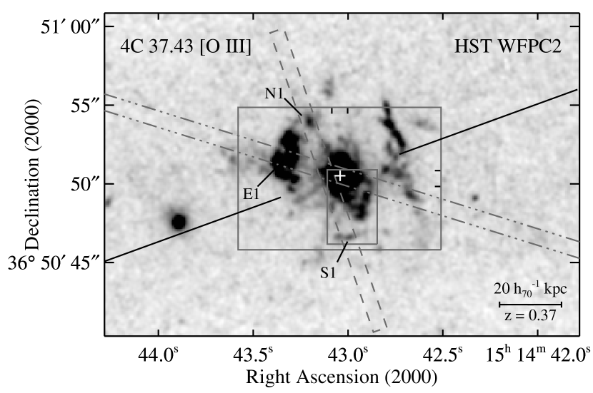
Figure 1.— Hubble Space Telescope (HST) WFPC2 [O iii] image of 4C 37.43 (Stockton et al., 2002). Overlaid are the field-of-view (FOV) of the mosaicked GMOS IFU2 datacube (outer solid box), the field of the GMOS IFUR datacube (inner solid box), the position of the DEIMOS slit (long dashed rectangle) and that of the LRIS slit (long dash dotted lines). The tick marks on the inner edge of the total IFU2 FOV show the overlapping regions of the four IFU2 pointings; from each corner, the rectangle defined by the farthest tick mark from the corner gives the FOV for a single pointing. The radio jet direction is described by the solid lines. The cross near the center marks the position of the QSO.

4C 37.43 has the most luminous EELR among QSOs at $z\leq 0.45$ (Stockton & MacKenty, 1987). The continuum image of the host galaxy shows distortions and a likely tidal tail that indicate that a major merger is in progress, which has probably triggered the current episode of quasar activity. Like most others, this EELR is morphologically completely uncorrelated with both the stellar distribution in the host galaxy and with the FR II double radio source (Miller et al., 1993). It has two main condensations of ionized gas at roughly the same distance ($\sim$3.5″, i.e., about 18 kpc) to the east and west of the quasar (Fig. 1). The optical spectrum of the brightest region, the main east condensation (E1; following Stockton et al. 2002), has been discussed in several papers before (Stockton, 1976; Boroson & Oke, 1984; Stockton et al., 2002). Here we present our new GMOS integral field spectroscopy and DEIMOS longslit spectroscopy covering a large fraction of the whole EELR. Throughout we assume a flat cosmological model with $H_{0}=70$ km s^-1 Mpc^-1, $\Omega_{m}=0.3$, and $\Omega_{\Lambda}=0.7$.

2. Observations and data reduction

2.1. GMOS Integral Field Spectroscopy

4C 37.43 was observed with the Integral Field Unit (IFU; Allington-Smith et al. 2002) of the Gemini Multiobject Spectrograph (GMOS; Hook et al. 2004) on the Gemini North telescope. We observed a $13\arcsec\times 9\arcsec$ region centered on the QSO in the early half-night of 2006 May 23 (UT). Since the main purpose of these observations was to determine the global velocity field of the EELR through the [O iii] $\lambda$5007 line, the IFU was used in the full-field (two-slit) mode and dithered on a rectangular grid of $6\arcsec\times 4\arcsec$. The QSO was successively placed at each corner of the $7\arcsec\times 5\arcsec$ IFU field and $\sim$0$\farcs$5 away from the edges, so the fields covered by the pointings overlap with each other by $\sim$1″ (see Fig. 1). We obtained two 720-s frames and one 156-s frame on the SE pointing and three 720-s exposures on the other three pointings. With the R831/G5302 grating and a central wavelength of 658.5 nm, we obtained a dispersion of 0.34Å per pixel, a spectral resolution of $\sim 1.3$Å (58 km s^-1) FWHM, and a wavelength range of 6330–6920 Å. The $r$ and RG610 filters were used to avoid spectral overlaps. The spectrophotometric standard star Feige 34 was observed for flux calibration. The seeing was $\sim 0\farcs 4$ throughout the half-night. Before running the data through the reduction pipeline (see the 3rd paragraph in this section), the exposures for each pointing position were combined using the IRAF task IMCOMBINE. We weighed the frames according to their integration times. Pixels were rejected if their values were 7-$\sigma$ off the median. For all four positions, there are no apparent cosmic rays in the final image. The shortened exposure of the SE pointing did make the data a little bit shallower in this region than others. We corrected for this difference by using an exposure map while making the final mosaicked datacube.

We also obtained deep integral field spectroscopy on a $\sim 3\farcs 5\times 5\arcsec$ region about 2″ SW of the QSO. A total of five 2400-s exposures were taken with the half-field (one-slit) mode in the first half-night of 2006 May 24 (UT). This configuration provides a wider spectral coverage but a smaller field than does the two-slit mode. With the B600/G5303 grating and a central wavelength of 641.2 nm, the dispersion and spectral resolution were approximately 0.46Å per pixel and 1.8Å (FWHM). The wavelength range was 4250–7090 Å, which includes emission lines from [Ne v] $\lambda$3426 to [O iii] $\lambda$5007. BD +28° 4211 was observed for flux calibration. The seeing was $\sim$0$\farcs$6 during the half-night.

The data were reduced using the Gemini IRAF package (Version 1.8). The data reduction pipeline (GFREDUCE) consists of the following standard steps: bias subtraction, cosmic ray rejection, spectral extraction, flat-fielding, wavelength calibration, sky subtraction, and flux calibration. Spectra from different exposures were assembled and resampled to construct individual datacubes (x,y,$\lambda$) with a pixel size of 0$\farcs$05 (GFCUBE). For each datacube, differential atmosphere refraction was corrected by shifting the image slices at each wavelength to keep the centroid of the quasar constant. The four datacubes resulting from the four IFU two-slit pointings were then merged to form a single datacube (the IFU2 datacube), and the five datacubes from the IFU one-slit mode were combined to form the IFUR datacube. Finally, these two datacubes were binned to 0$\farcs$2 pixels, which is the original spatial sampling of the IFU fiber-lenslet system.

Since our study focuses on the emission-line gas, it is desirable to remove the light of the quasar from the datacubes. Since the emission-line clouds show essentially pure emission-line spectra, we used the continuum on either side of an emission line to precisely define the PSF of the quasar. We then ran the two-component deconvolution task PLUCY (contributed task in IRAF; Hook et al. 1994) on each image slice across the emission line to determine the flux of the quasar at each wavelength. Finally the quasar component was removed by subtracting a scaled PSF (according to the fluxes determined by PLUCY) from each image slice. Note that the deconvolved images produced by PLUCY were not used to form the QSO-removed datacubes.

2.2. DEIMOS Longslit Spectroscopy

We obtained additional longslit spectroscopy using the DEep Imaging Multi-Object Spectrograph (DEIMOS; Faber et al. 2003) of the Keck II telescope on 2006 August 28 (UT). We initially centered the 20″ long slit on the QSO at a position angle of 19^∘ (N to E), then offset it by 0$\farcs$73 so that it goes through two EELR clouds (N1 & S1; Fig. 1) that are presumably associated with X-ray emission (see Fig. 5 in Stockton et al. 2006a). The alignment accuracy of DEIMOS is typically $\sim$0$\farcs$1. The total integration time was 3600 s. With a 600 groove mm^-1 grating, a $0\farcs 9$ wide slit and a central wavelength at 7020Å, we obtained a dispersion of 0.63 Å per pixel, a resolution of 3.5 Å, and a spectral range of 4570–9590 Å, covering emission lines from [Ne v] $\lambda$3346 to [S ii] $\lambda$6731. The spectrophotometric standard star Wolf 1346 was observed with a 1$\farcs$5 wide slit at parallactic angle. The GG400 filter was used for all observations. The seeing was $\sim 0\farcs 7$ during the observations. We reduced the data using the $spec2d$ data reduction pipeline. The standard star spectrum suffers second-order contamination in the spectral range $\gtrsim$ 8000 Å; for the spectra of the EELR this contamination is negligible since there is essentially no continuum. However, in order to flux calibrate the emission-line spectra, one needs to correct for the second-order contamination of the standard star spectrum. We thus obtained a DEIMOS spectrum of Feige 34 taken on November 29 2006 (UT). This standard star was observed using the same settings as ours except that a different filter (GG495) and a slightly different central wavelength were used. Since both GG400 and GG495 filters reach an identical transmission value redward of 7000 Å, no correction for the transmission curves needs to be applied. We first derived the calibration files with STANDARD for both spectra, then multiplied the Feige 34 data by a constant so that the two matched between 7000 and 7600 Å. Then, in the bluer region, we selected the data points from the GG400 spectrum (Wolf 1346), while in the redder region, we selected the GG495 data (Feige 34). We then fitted a smooth curve to the selected data to form the final sensitivity function (SENSFUNC), which was used in the flux calibration.

Proper sky subtraction is often a problem beyond 7000 Å because of strong airglow lines and fringing in the CCD. The $spec2d$ pipeline attempts to defringe the spectra by dividing the science spectra with a normalized flat field. This feature significantly improves the sky subtraction result, although it is still not perfect when dealing with the strongest sky lines. Fortunately, the redshift of 4C 37.43 nicely places the important red lines (i.e., [N ii] $\lambda\lambda$6548,6584, H$\alpha$ and [S ii] $\lambda\lambda$6717,6731) in a window (8900–9300 Å) between two strong OH bands that is essentially free of strong sky lines, making the subtraction of sky lines almost perfect in this region.

Figure 1 presents an overview of the regions covered by the observations discussed above. We also include a deep Keck I LRIS (Low-Resolution Imaging Spectrometer; Oke et al. 1995) spectrum from Stockton et al. (2002) in our discussion. That spectrum had a total integration of 3600 s and was taken with a 300 groove mm^-1 grating and a 1″ wide slit. The position of this slit is also shown in Fig. 1.

3. Results

3.1. Kinematics

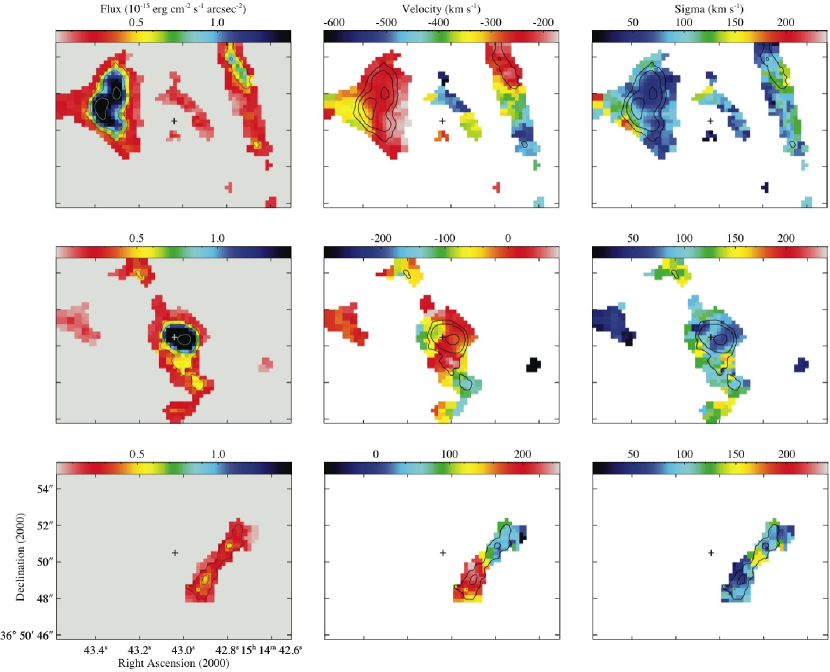
Figure 2.— Velocity field of 4C 37.43 EELR derived from the [O iii] $\lambda$5007 region of the QSO-subtracted IFU2 datacube. The three columns, from left to right, are line intensity, radial velocity (relative to that of the nuclear NLR) and velocity dispersion maps. To separate different clouds that are present along the same line of sight, the velocity field is shown in three separate velocity bands ($-$620 to $-$170 km s^-1, $-$290 to +80 km s^-1 and $-$70 to +250 km s^-1 from top to bottom), and the line intensity and velocity dispersion maps refer to the same clouds. Pixels are 0$\farcs$2 squares. The crosses indicate the position of the quasar before it was removed from the datacube (for details see § 2.1). Contours are from the line intensity maps.

Figure 2 presents the velocity field of the [O iii] $\lambda$5007 emission derived from the IFU2 datacube, which has a spectral range that brackets the H$\beta$–[O iii] region. The QSO was removed from the datacube using the method described in § 2.1. We discarded spectra that show very low amplitude-to-noise ratios (A/N $\leq$ 3), and spatially binned the remaining spectra with A/N $\leq$ 10 to a target A/N $\approx$ 8 using the Voronoi binning method of Cappellari & Copin (2003). We then used multiple Gaussians to fit the [O iii] $\lambda$5007 line profile in the binned datacube. Because different velocity components are sometimes present along the same line of sight, the velocity field is displayed in three velocity bands from $-$620 to +250 km s^-1(relative to $z_{0}=0.37120$, the redshift of the quasar NLR as determined from its [O iii] $\lambda\lambda$4959,5007 lines). The velocity dispersion ($\sigma$) measurements were corrected for the $\sigma_{0}=24.6$ km s^-1 instrumental resolution. Monte-Carlo simulations were performed to determine the uncertainties in the measured line parameters. For A/N = 8 and an intrinsic $\sigma=50$ km s^-1 (130 km s^-1), the 1-$\sigma$ errors on velocities ($V$) and velocity dispersions ($\sigma$) are both about 4 km s^-1(6 km s^-1), and the errors on fluxes are about 6% (4%).

Our velocity maps are generally consistent with those from previous integral-field spectroscopy and image-sliced spectroscopy (Durret et al., 1994; Crawford & Vanderriest, 2000; Stockton et al., 2002), but they offer a much clearer view of the complexities in the velocity structure of this region. Overall, these maps show that: (1) the clouds comprising the EELR are certainly not in a coherent rotation about the QSO, as already pointed out by Stockton (1976) with very limited velocity information; (2) the majority of the clouds are blueshifted relative to the QSO, and the highest blueshifted velocity is about $-$620 km s^-1, while the highest redshifted velocity is only +250 km s^-1; (3) the velocity dispersions for the most part are between 50 and 130 km s^-1(or 120 to 310 km s^-1 FWHM), much higher than the sound speed in a hydrogen plasma at $10^{4}$ K, $c_{s}\sim$ 17 km s^-1; (4) there is no obvious evidence for jet-cloud interactions. As seen in Fig. 1, the radio jet just misses the two major condensations, and no significant increase in velocity dispersion is observed where the jet crosses any visible part of a cloud.

As shown in the $-620$ to $-170$ km s^-1 panels, the two major condensations to the east (E1) and west of the QSO are both blueshifted to about $-250$ km s^-1. E1 is resolved in our velocity maps, thanks to the 0$\farcs$2 sampling of the IFU and the 0$\farcs$4 seeing. The southern half of E1 shows a velocity increase from $-$180 to $-$350 km s^-1 along the W-E direction, and also an increase in $\sigma$ from 50 to 110 km s^-1 along the same direction. This kinetic structure suggests that E1 is not a coherent body (first suspected by Durret et al. 1994); instead, it is composed of sub-clouds, as clearly seen in the HST [O iii] image (see the low-contrast insets to Fig. 3 of Stockton et al. 2002).

Overall, the velocity field of the 4C 37.43 EELR is similar to that of the EELR around 3C 249.1 (Fu & Stockton, 2006), in the sense that both of them appear globally chaotic but locally ordered.

3.2. Electron Density and Temperature

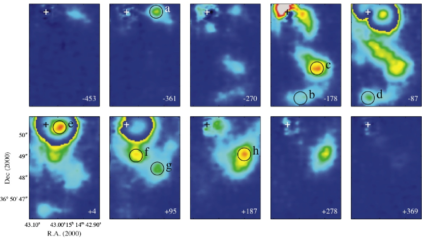
Figure 3.— [O iii] $\lambda$5007 radial velocity channel maps from the QSO-subtracted IFUR datacube. The central velocities, in km s^-1 relative to that of the quasar NLR, are indicated in the lower-right corner of each panel. The circles show the extraction apertures of the various emission-line clouds discussed in the text. Some of the images have been allowed to wrap around to show both low surface brightness detail and high surface brightness peaks. The crosses indicate the position of the QSO before it was removed from the datacube.

Our IFUR datacube covers the [O ii] $\lambda\lambda$3726,3729 doublet, and its spectral resolution ($\sim$1.8Å) is high enough to resolve the two. We can determine the [O ii] luminosity-weighted average electron densities ($N_{e}$[O ii]) from the intensity ratio of the doublet (Osterbrock, 1989). Electron temperatures ($T_{e}$) can be measured using the [O iii] ($\lambda$4959+$\lambda$5007)/$\lambda$4363 ratio (R_OIII). Most of the clouds in the IFUR field-of-view (FOV) have a low surface brightness, making it impossible to reliably measure the line ratios from a single 0$\farcs$2 pixel. We therefore identified the peaks of the individual clouds, then binned pixels within $0\farcs 3$ of the peak. Figure 3 displays the extraction apertures for the eight resolved clouds.

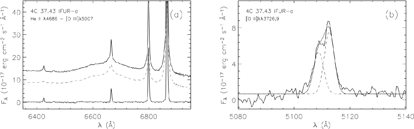
Figure 4.— Spectra of 4C 37.43 EELR e extracted from the IFUR datacube. (a) The He ii $\lambda 4686$ to [O iii] $\lambda 5007$ portion of the spectra. The upper and lower solid curves are the extracted spectra before and after removing the QSO from the datacube. The dashed curve shows the difference between the two, i.e., the scattered light from the QSO. For clarity, the dashed curve was shifted downward by $5\times 10^{-17}$ erg cm^-2 s^-1 Å^-1. (b) The [O ii] $\lambda\lambda$3726,9 doublet of the EELR e. QSO scattered light has been removed. The dashed curves show the decomposition of the doublet, and the smooth solid curve is the sum of the two.

Figure 4a compares the extracted spectra from cloud $e$ before and after removing the QSO from the datacube (§ 2.1). It shows that the PSF subtraction technique can successfully remove the QSO scattered light even for a cloud only 0$\farcs$6 from the quasar, as confirmed by the absence of the broad H$\beta$ line in the residual spectrum. Note that since the data were taken under excellent seeing condition ($\sim 0\farcs 6$), PSF subtraction is only critical for the clouds very close to the quasar, namely $a$, $e$, and $f$. In addition, the line ratios for clouds $a$ and $f$ should be reliable even if the QSO removal were just barely correct, because the two are well separated from the quasar NLR in velocity. We are less confident about the line ratios of cloud $e$, since its velocity is almost centered on that of the NLR. However, the shape of the cloud as seen in the residual datacube (see Fig. 3 as an example) suggests that the PSF removal cannot be too far off. Also at least the [O ii] ratio should be trustworthy since the NLR emits very weakly in this doublet.

To estimate the effect of using a fixed-size aperture on the covering fraction of the PSF (since the spatial resolution gets better as the wavelength increases), we compared a QSO spectrum extracted from a $d=4\farcs 8$ aperture with another one from a $d=0\farcs 6$ aperture. A smoothed version of the ratio of the two was used to correct for the spectra of all the emission-line clouds. The atmospheric B-band absorption was corrected by dividing the spectra by an empirically determined absorption law. The Galactic extinction on the line of sight to 4C 37.43 is $A_{V}$ = 0.072 (Schlegel et al., 1998). Intrinsic reddening due to dust associated with the cloud, whenever possible, was determined from the measured H$\gamma$/H$\beta$ ratio assuming an intrinsic ratio of 0.468 (for case B recombination at T = $10^{4}$ K and $N_{e}=10^{2}$ cm^-3; Osterbrock 1989). However, there are four clouds, namely $a,b,d,$ and $g$, where H$\gamma$ is not securely detected in the IFU data. For clouds $b$ and $d$, we used the reddening implied by the H$\gamma$/H$\beta$ ratio from the DEIMOS spectrum of S1 (Fig. 1). For $a$ and $g$, we assumed an arbitrary reddening of $A_{V}=0.7$. Both reddening effects were corrected using a standard Galactic reddening law (Cardelli et al., 1989).

To measure the line ratios of the [O ii] doublet, we used two Gaussian profiles constrained to be centered on the expected wavelengths of the doublet after applying the same redshift. As an example, Fig. 4b shows the profile of the [O ii] doublet for the cloud $e$ and the best two-Gaussian model fit. For the cases where there are two velocity components in a single spectrum, we first identify which component corresponds to the target cloud and which one is from contaminating light from other nearby clouds. Then we measure the velocity difference between the two from the [O iii] $\lambda\lambda$4959,5007 lines. Finally we freeze this parameter when fitting other lines, including the [O ii] doublet. For the DEIMOS spectra of N1 and S1, the [O ii] doublet is unresolved, so we measured the density-sensitive [S ii] $\lambda$6716/$\lambda$6731 ratios.

When there is a good [O iii] $\lambda$4363 line measurement, we derived $T_{e}$ and $N_{e}$ consistently using the IRAF routine TEMDEN. Otherwise, a uniform $T_{e}=10^{4}$ K was assumed. $N_{e}$[O ii]($N_{e}$[S ii]) would be approximately 15% (5%) higher, if $T_{e}$ = 15000 K.

The physical properties of the EELR clouds are summarized in Table 1. The listed [O iii] $\lambda$5007 velocity dispersions have been corrected for the instrumental broadening ($\sigma_{0}\approx 35$ km s^-1 for IFUR; $\sigma_{0}\approx 67$ km s^-1 for DEIMOS). Reddening-free emission-line fluxes and 3-$\sigma$ upperlimits are tabulated in Table 2 as ratios to the H$\beta$ flux. The quoted 1-$\sigma$ errors were derived from the covariance matrices associated with the Gaussian model fits, with the noise level estimated from line-free regions on either side of an emission line. For completeness, we have also included E1 in both tables. Most of the line fluxes were re-measured from the LRIS spectrum except for the [O ii] doublet ratio, which is quoted from Stockton et al. (2002).

In general, the temperatures of the clouds are about 15000 K, and the densities are a few hundreds cm^-3. The cloud $e$ looks peculiar in this crowd: it has both the coolest temperature and the lowest density, implying a pressure much lower than the average. The only other low-density cloud is N1, where the [S ii] ratio is at the low-density limit.

3.3. Ionization Mechanisms

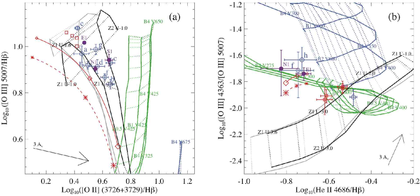
Figure 5.— Line ratio diagnostic diagrams distinguishing different ionization mechanisms: (a) [O ii] $\lambda\lambda 3726,9$/H$\beta$ vs. [O iii] $\lambda 5007$/H$\beta$, (b) He ii $\lambda 4686$/H$\beta$ vs. [O iii] $\lambda 4363$/[O iii] $\lambda 5007$, and (c) [O ii] $\lambda\lambda 3726,9$/[Ne iii] $\lambda 3869$ vs. [O iii] $\lambda 5007$/H$\beta$. Overplotted are model grids from the dusty radiation-pressure dominated photoionization model (black and grey; Groves et al. 2004), shock-only (blue) and “shock + precursor” models (green; Dopita & Sutherland 1996), along with the two-component photoionization sequences with two different abundance sets (red lines with symbols). The dusty photoionization grids cover a range of ionization parameters (log($U$)) for metallicities of 1.0 and 2.0 $Z_{\odot}$, and two power-law indexes for the ionizing continuum (black grids for $\alpha=-1.2$, and grey ones for $\alpha=-1.4$). In the shock models, a range of shock velocities ($V_{S}$ [km s^-1]) and magnetic parameters ($B/n^{1/2}$ [$\mu$ G cm^-3/2] ) are covered. The two-component photoionization sequences show a range of combination ratios between the two components. The dashed and solid red lines represent the models adopting gas abundance set $a$ and set $b$, respectively (see § 3.3 for details). The asterisks and diamonds, with increasing sizes, denote the positions where 20, 50 and 80% of the total H$\beta$ flux is from the high-density IB component. Line ratio measurements from the 4C 37.43 IFUR datacube are shown as blue open circles, and purple filled circles show the measurements from either LRIS (E1) or DEIMOS (N1 & S1) longslit spectra. For comparison, the four EELR clouds of 3C 249.1 (Fu & Stockton, 2006) are plotted as red open squares. Arrows are reddening vectors.

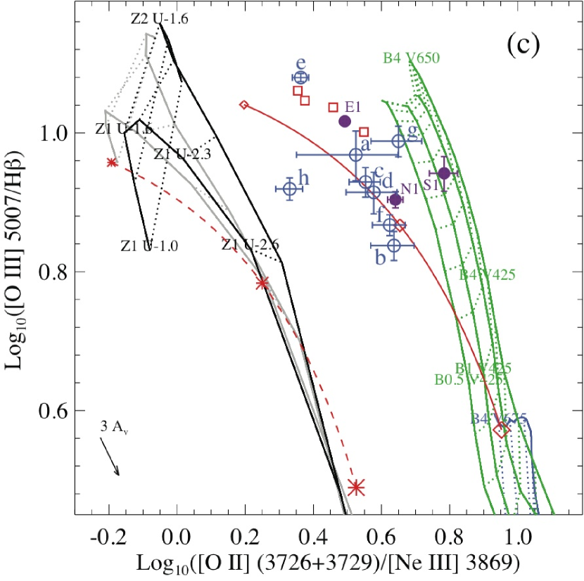
Figure 5.— continued

Line ratio diagnostic diagrams are widely used to distinguish different ionization mechanisms and to infer useful physical parameters of ionized clouds. Figure 5 presents three of these diagrams. Our line-ratio data are plotted against four ionization models, which were all computed by the multipurpose photoionization-shock code MAPPINGS: (1) a dusty radiation-pressure dominated photoionization model (Groves et al., 2004), (2) a two-phase photoionization model, (3) a shock ionization model and (4) a “shock + precursor” model (Dopita & Sutherland, 1996).

These diagrams clearly show that both pure shock and “shock + precursor” are not as successful as the photoinozation models in reproducing the observed spectra of the EELR. At first sight, Fig. 5a might seem to imply that the “shock + precursor” model would possibly fit the data if we weight the precursor component more heavily. However, the high shock velocities ($>$ 400 km s^-1) required to reach the observed high [O iii]/H$\beta$ ratios are inconsistent with the measured low velocity dispersions of those clouds (Fig. 2). In addition, making the precursor more luminous would only move the grids below where they are in Fig. 5b, hence further off the data points. Therefore, we believe that it is unlikely that any of these clouds are dominated by shock ionization; instead, they are photoionized by the central QSO. In fact, it was argued before that at least E1 was photoionized by the QSO, as indicated by the low intensity ratios of O iv $\lambda 1402$/He ii $\lambda 1640$ and C iv $\lambda 1549$/He ii (Stockton et al., 2002).

Briefly, Model 1 simulates the photoionization of the surface layer ($\lesssim$ a few pc) of a dense self-gravitating molecular cloud, where the hydrogen density near the ionization front is about 1000 cm^-3 and the density structure is predominantly determined by radiation pressure forces exerted by the absorption of photons by gas and dust. Detailed discussions of this model can be found in Groves et al. (2004).

The two-phase photoionization model is similar to the $A_{M/I}$ model by Binette et al. (1996). It assumes that the observed emission-line spectrum is a combination of the emission from two species of clouds. Guided by the results of Stockton et al. (2002), we used the latest version of MAPPINGS (3r) to model two isobaric components: (1) a high-excitation matter-bounded (MB) component with a density $N_{H}\sim 1$ cm^-3, a temperature $T\sim 1.5\times 10^{4}$ K and an average ionization parameter $U\sim 6\times 10^{-2}$, and (2) a low-excitation ionization-bounded (IB) component with $N_{H}\sim 400$ cm^-3, $T\sim 10^{4}$ K and $U\sim 2\times 10^{-4}$. Unlike the $A_{M/I}$ model, shielding of the ionizing source by the MB component is not considered, i.e.,  both clouds are facing the same ionization field. Different combination ratios of the two components produce a sequence of spectra. We show in the diagrams a range of models having 20 to 80% of the total H$\beta$ flux from the high-density IB component.

Both photoionization models used simple power laws to represent the ionizing continuum ($F_{\nu}\propto\nu^{\alpha}$). Model 1 assumed a single-index power-law from 5 to 1000 eV, and we show here two index values Groves et al. (2004) modelled, $\alpha=-1.2,-1.4$. Model 2 uses a more realistic segmented power-law with $\alpha=-1.5$ in the UV (8–185 eV) and $\alpha=-1.2$ in the X-ray (185–5000 eV). The ionizing flux at the Lyman limit is normalized to $3.3\times 10^{-17}$ erg cm^-2 s^-1 Hz^-1 (Stockton et al., 2002). These indexes are close to the canonical value proposed for the typical spectral-energy distribution of a QSO (i.e., $\alpha=-1.4$; e.g., Ferland & Osterbrock 1986).

We have run our two-phase model on two different sets of abundances: (a) the same dust-depleted 1 $Z_{\odot}$ abundance set as used in Model 1 (Groves et al., 2004); (b) the “standard” Solar abundance set ($Z^{{}^{\prime}}_{\odot}$) of Anders & Grevesse (1989) scaled by $-0.5$ dex, following Stockton et al. (2002). Note that the total gas metallicities in the two sets are both around one-third of $Z^{{}^{\prime}}_{\odot}$. Table 3 compares the two abundance sets. Sequences from both runs are shown in Fig. 5. In all diagrams, set $b$ clearly provides a superior fit to the data than set $a$, meaning that the gas abundance in those clouds is more similar to $Z^{{}^{\prime}}_{\odot}$. It also explains why there is a drastic offset between the data and the grids from Model 1 in Fig. 5c. Therefore, hereafter the two-phase model (or Model 2) only refers to the run using abundance set $b$.

Figure 5a shows that both photoionization models can reproduce the strong oxygen lines, since such line ratios are mainly determined by the average ionization parameter. But the two begin to disagree in Fig. 5b, where weaker lines like He ii $\lambda 4686$ and [O iii] $\lambda 4363$ are involved. This discrepancy arises because of the different density structures of the modeled clouds. In the dusty model (Model 1) the hydrogen density in a cloud varies from a few hundreds to $\sim$1000 cm^-3. In this diagram, Model 1 cannot provide a good fit to the data unless an extremely low metallicity ($\lesssim 0.2Z_{\odot}$) is used, which nonetheless contradicts the best fit grids in Fig. 5a and Fig. 6 (§ 3.4). However, the low-density MB component in the two-phase model can easily reproduce both the high temperature ($\sim$ 15000 K) and the low He ii fluxes. Since most of the [O iii] is emitted by the MB cloud, the influence from the IB cloud on temperature is negligible. We emphasize that the high-density IB component is indispensible to achieve the overall best fit, because the high [O ii] fluxes cannot be explained by the high-excitation MB component alone. Note that since the emission lines involved in these diagrams are fairly insensitive to density effects, lowering density in the dusty model has the same effect as increasing the ionization parameter, and hence would not improve the fit to the data.

The failure of Model 1 shows that these clouds are probably not as dense as a giant molecular cloud (GMC). In fact, as argued by Stockton et al. (2002), the general lack of correlation between the morphology of the EELR and that of the stars in the host galaxy argues against them being GMCs, since GMCs are supposedly dense enough that their trajectories should follow those of the stars and not be affected seriously by hydrodynamic interactions.

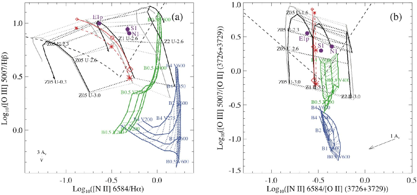
Figure 6.— Metallicity sensitive diagnostic diagrams — (a) [N ii] $\lambda 6584$/H$\alpha$ vs. [O iii] $\lambda 5007$/H$\beta$, (b) [N ii] $\lambda 6584$/[O ii] $\lambda\lambda 3726,9$ vs. [O iii] $\lambda 5007$/[O ii] $\lambda\lambda 3726,9$. Keys are the same as in Fig. 5. The photoionization girds here display a smaller range of ionization parameters but a wider range of metallicities (0.5, 1.0 and 2.0 $Z_{\odot}$). In panel a the dashed black curve is the empirical starbursts/AGN dividing line (Kewley & Dopita, 2002), and in panel b the dashed black lines are the empirical cuts used by Groves et al. (2006) to select the lowest metallicity Seyfert 2s ($Z\sim 1Z_{\odot}$). In both panels, the top regions bordered by the dashed black curve/lines are where the low-metallicity Seyfert 2s are located.

The success of the simple two-phase model suggests that these clouds consist of a general low-density medium together with a clumpy distribution of much denser gas. This picture is also supported by the amount of reddening and the density-sensitive line ratios observed in these clouds (Table 1). An intrinsic reddening of $A_{V}\sim 0.6$ mag is generally seen in such clouds, which implies a hydrogen column density of $\sim 10^{21}$ cm^-2. Assuming that the depth along the line-of-sight of the clouds is comparable to the resolved width of E1 (1″ $\sim$ 5 kpc), the resulting number density is $\sim$0.1 cm^-3. But we constantly measure a few hundreds cm^-3 from either [O ii] or [S ii] ratios. A natural solution to this apparent contradiction is that clumpy dense clouds coexist with a much more diffuse medium. The former produces most of the low-ionization emission lines such as the [O ii] $\lambda\lambda$3726,3729 and [S ii] $\lambda\lambda$6717,6731 doublets, leading to the measured high densities; but the latter holds most of the mass. As pointed out by Stockton et al. (2002), the dense clouds need to be continuously supplied, possibly through compression of the diffuse medium by low-speed shocks, because (1) the two kinds of clouds are not in pressure equilibrium since the temperatures of the two are both around $10^{4}$ K, and (2) the denser clouds are geometrically thin ($\sim$0.1 pc, at least for the ionized part), thus cannot be stable on a timescale longer than $10^{4}$ yr, given a typical sound speed of $\sim$ 17 km s^-1. We will discuss the origin of the high-density medium in more detail in § 4.2.

3.4. Metallicity

Diagrams involving the metallicity sensitive [N ii] $\lambda 6584$ line are shown in Figure 6. The only clouds where we have spectral coverage reaching the H$\alpha$-[N ii] region are those observed with DEIMOS (N1 and S1). Although the two clouds are about 40 kpc apart in projected distance, their line ratios fall very close in Fig. 6, suggesting similar metallicities. Boroson & Oke (1984) presented emission-line fluxes (their Table 2) of an E1 spectrum that covered the H$\alpha$-[N ii] region. After dereddening, their data are consistent with the line ratios we measure from the LRIS spectrum of E1. Because of their limited spectral resolution, they only listed the total flux from H$\alpha$ + [N ii] $\lambda\lambda$6548,6584. We roughly decomposed the H$\alpha$ and [N ii] $\lambda 6584$ fluxes by assuming the case B value of H$\alpha$/H$\beta$ = 2.9 and a theoretical ratio of the [N ii] doublet of 3.0. The line ratios of this region are also plotted in Fig. 6 (labeled as “E1p” to distinguish from the E1 region represented by the LRIS spectrum).

The fact that different photoionization models with a same abundance fall precisely onto one another in these plots shows that such line ratios are almost entirely dependent on the abundance. Therefore, the grids from the dusty model (Model 1) can be used to measure the metallicities of the EELR clouds, even though it cannot reproduce some of the line ratios (refer to § 3.3).

By interpolating the grids of Model 1 in both panels of Fig. 6, we estimated that 12 + log(O/H) = 8.55, 8.58, 8.42 for S1, N1 & E1p, respectively (Hereafter we will refer to 12 + log(O/H) as (O/H)). Since the metallicity determination also slightly depends on the density and Model 1 used a density of $\sim$1000, we have corrected the above values using the densities listed in Table 1 and the approximate (O/H) $\propto$ log($N_{e}$) scaling given in the Eqn. [4] of Storchi-Bergmann et al. (1998). The metallicities after the correction are (O/H) = 8.62, 8.68, 8.47 for S1, N1 & E1p, respectively. The lower metallicity of E1p indicates that there might be some metallicity variations within an EELR.

Storchi-Bergmann et al. (1998) obtained two abundance calibrations for AGN NLRs from photoionization models. The calibrations involve similar line ratios as those in Fig. 6, and were shown to yield consistent abundance values with those from H ii regions for a sample of Seyferts. Therefore it is reassuring that the abundances obtained from these two calibrations are consistent with our simple interpolated results. The average of the two abundance calibrations of Storchi-Bergmann et al. (1998) (their Eqs. [2], [3] and [4]) gives (O/H) $\simeq$ 8.64, 8.68 and 8.54 for S1, N1 and E1p, respectively.

To compare the data with the Seyferts at similar redshifts from the Sloan Digital Sky Survey (SDSS), we delineated the regions where the lowest metallicity Seyfert 2s were found in SDSS spectroscopic galaxy sample (Groves et al., 2006) in Fig. 6. The regions are on the left side of the main Seyfert branch in both panels. It is clear that the three EELR clouds around 4C 37.43 all show significantly lower metallicities than typical NLRs of Seyferts ((O/H) $\gtrsim 8.8$; Groves et al. 2006).

4. Discussion

4.1. The Low Metallicity of 4C 37.43

Quasars are usually found in metal-rich environments ((O/H) $\gtrsim$ (O/H)${}^{{}^{\prime}}_{\odot}$ = 8.93) (e.g., Hamann et al. 2002). The metallicity does not show a correlation with redshift, but seems to increase with black hole (BH) masses (Warner et al., 2003). The BH mass in 4C 37.43 is about 10⁹ M_⊙ (Labita et al., 2006), which predicts (O/H) = 9.8 (Warner et al., 2003). However, the low flux ratios of N v $\lambda 1240$/C iv $\lambda 1549$ ($\sim$ 0.04) and N v/He ii $\lambda 1640$ ($\sim$ 0.24) observed in the broad-line region (BLR) of this quasar (Kuraszkiewicz et al., 2002) both indicate a significantly lower metallicity, (O/H) $\approx$ 8.4 (i.e., about 20 times lower than a typical quasar with $M_{BH}$ = 10⁹ M_⊙) according to the theoretical predictions of Hamann et al. (2002). Nevertheless, this BLR metallicity is close to those measured in the surrounding EELR (§ 3.4).

This low metallicity is unexpected for a quasar with a BH mass of 10⁹ M_⊙ if (1) the bulge-mass—BH-mass and the bulge-mass—metallicity correlations hold for this object and (2) the gas in the BLR and the EELR is from the ISM of the host galaxy of the quasar. There is no indication that the host galaxy of 4C 37.43 is particularly low mass: it is easily visible in ground-based and HST imaging (Stockton et al., 2002), and, in fact, Labita et al. (2006) find that the BH mass for 4C 37.43 from the host galaxy luminosity falls nicely between BH masses from the broad emission line widths calculated under two different assumptions regarding the geometry of the BLR (see their Table 4).

Thus, whatever mechanism establishes the bulge-mass—BH-mass correlation likely was in operation in 4C 37.43 long before the current episode of quasar activity, and the BH almost certainly underwent most of its growth phase early on. The low metallicity of the gas in the BLR and EELR therefore indicates that this gas has come from an external source, most likely a late-type gas-rich galaxy that has recently merged. If this is true, it provides the first direct observational evidence that gas from a merger can find its way down to the very center of the merger remnant, to within fueling distance of the active nucleus, although there has been a compelling statistical argument that this is the case for at least some QSOs (Canalizo & Stockton, 2001).

4.2. The Origin of the High-Density Medium

The viscosity of a fully ionized hydrogen plasma at $N_{e}$ = 1 cm^-3 and $T=10^{4}$ K is $\mu\approx 9.5\times 10^{-7}$ g s^-1 cm^-1 (Spitzer, 1962). Such a low viscosity implies a large Reynolds number if the scale and the speed of the flow are large. In fact, for a typical EELR cloud, R = $Vm_{p}Nl/\mu$ $\approx$ 10¹¹, given a flow velocity $V$ = 200 km s^-1, a number density $N$ = 1 cm^-3 and a typical length scale $l$ = 1 kpc. This means that turbulent motions can be easily triggered if the clouds are moving, converting part of its bulk kinetic energy into turbulent energy.

The observed line-widths are around $\sigma\sim 50$ km s^-1, while the sound speed in an ionized hydrogen plasma at $10^{4}$ K is only $c_{s}$ $\sim$ 17 km s^-1. Shocks with a velocity $\sim$50 km s^-1 must be common inside the cloud. If the pre-shock gas is $10^{4}$ K, an isothermal shock with a speed of 50 km s^-1 is able to compress the gas by only a factor of 10 ($\rho_{2}/\rho_{1}=M^{2}$, where $M$ is the Mach number). But if the pre-shock gas is shielded from the ionizing source by the compressed post-shock gas, then the temperature of the pre-shock gas is probably $\sim$100 K, which corresponds to a sound speed of just $\sim$2 km s^-1. The same shock speed thus could increase the gas density by over 600 times, sufficient to explain the high density contrast ($\sim$300) between the two phases, as required by our best fit photoionization model (§ 3.3). The total mass in the dense medium can stay relatively stable as long as the mass loss rate due to thermal expansion is comparable to the mass accretion rate through shock compression. We note that the amount of neutral gas due to this self-shielding should be inappreciable compared to the total mass of the cloud, since the filling factor of the dense material is known to be minuscule ($\phi\sim 10^{-5}$; Stockton et al. 2002). Also, for shocks at such a low speed, the amount of UV photons produced by the shock itself cannot significantly ionize the pre-shock neutral gas ($U\approx 6\times 10^{-5}$ for $V_{S}=50$ km s^-1 and $N=1$ cm^-3; Dopita & Sutherland 1996).

Supersonic turbulence decays rapidly, typically over a crossing timescale. However, since these clouds are large, the crossing time is in fact on the same order-of-magnitude as the dynamical timescale of the EELR, $\tau_{cross}\approx 20(l/1$ kpc)/($v_{t}/50$ km s^-1) Myr; so the picture of dense regions produced by shocks remains consistent with the timescales involved.

4.3. Mass of the Ionized Gas

The H$\beta$ luminosity of an ionized cloud is proportional to $N_{e}N_{p}V$, where $V$ is the volume occupied by the emitting material. So, if we assume $N_{H}$ = $N_{e}$ = $N_{p}$, then the total hydrogen mass can be derived once we have an estimate of $N_{e}$: $M$ = $4\pi m_{p}f_{\rm H\beta}d_{L}^{2}/(\alpha_{\rm H\beta}N_{e}h\nu)$ = $3.2\times 10^{8}$ $f_{\rm H\beta,-16}/N_{e,1}$ M_⊙, where $m_{p}$ is the proton mass, $d_{L}$ the luminosity distance, $\alpha_{\rm H\beta}$ the effective recombination coefficient of H$\beta$, $h\nu$ the energy of a H$\beta$ photon, $f_{\rm H\beta,-16}$ the H$\beta$ flux in units of $10^{-16}$ erg cm^-2 s^-1 and $N_{e,1}$ the electron density in units of 1 cm^-3. We assume a nominal density of 1 cm^-3 because, as argued in § 3.3, most of the mass is in the low-density medium with a density of $\sim$1 cm^-3 even though the electron densities measured from low-excitation lines are around hundreds cm^-3. The total mass of the entire EELR is $\sim$ $3\times 10^{10}$ M_⊙, given that the total H$\beta$ flux is $1\times 10^{-14}$ erg cm^-2 s^-1.

One can also infer the cloud mass from the amount of dust observed and a given dust-to-gas ratio. The dust column density is proportional to the amount of reddening we see along the line-of-sight. Assuming the Galactic dust-to-gas ratio, we obtain $M$ = $5.8\times 10^{21}$ cm^-2 mag^-1 E${}_{B-V}m_{p}d_{A}^{2}\theta^{2}$ = $4.0\times 10^{8}$ A_V $\theta^{2}$ M_⊙, where A_V is the intrinsic reddening in magnitude, $\theta^{2}$ is the solid angle subtended by the cloud in $\square\arcsec$. This result is consistent with what we obtained from the H$\beta$ luminosity if $N_{e}$ $\sim$ 1 cm^-3, validating the existence of the low-density medium. Taking this one step further, if we require the two masses to be consistent, then it is easy to show that $N_{e}$ = 0.8 ($f_{\rm H\beta,-16}$/$\theta^{2}$)/A_V cm^-3. The H$\beta$ surface brightness of the EELR peaks at $\sim 5\times 10^{-16}$ erg cm^-2 s^-1 arcsec^-2 for the brightest regions and at $\sim 1\times 10^{-16}$ erg cm^-2 s^-1 arcsec^-2 for more average clouds (Fig. 2; given an [O iii]/H$\beta$ ratio of 9). If we increase this value by a factor of 2 to account for the smearing due to seeing, we end up with $N_{e}$ $\lesssim$ 10 cm^-3 for the brightest clouds and $N_{e}$ $\lesssim$ 2 cm^-3 for the less luminous ones, given A_V = 0.8 mag.

The mass of the EELR is on the same order of magnitude as that of the total ISM in the Galaxy, which implies that perhaps almost the entire ISM of the quasar host galaxy (or, more likely, that of the merging partner) is being ejected as well as having been almost fully ionized by the quasar nucleus.

4.4. The Driving Source of the Outflow

The mass of the EELR, interpreted as an outflow, implies an enormous amount of energy. The bulk kinetic energy of the entire EELR is approximately $E_{KE}=MV^{2}/2=6.2\times 10^{57}M_{10}V_{250}^{2}$ ergs, where $M_{10}$ is the total mass in units of $10^{10}$ M_⊙ and $V_{250}$ = $V$/250 km s^-1. We used 250 km s^-1 as the nominal velocity scale because most of the mass is in the brightest two concentrations, which are both blueshifted by about 250 km s^-1. The kinetic energy of the unresolved kinematic substructures (“turbulent” energy) can be estimated from the measured line widths, $E_{tur}=M\sigma^{2}=5.0\times 10^{56}M_{10}\sigma_{50}^{2}$ ergs ($\sigma_{50}=\sigma/50$ km s^-1). The emission-line gas also has a thermal energy of $E_{TH}=1.5MkT/m_{p}=2.5\times 10^{55}M_{10}T_{4}$ ergs ($T_{4}=T(K)/10^{4}K$), which is just about 0.4% of the kinetic energy. Similarly, the total momentum is $p$ = $MV$ = $5\times 10^{50}M_{10}V_{250}$ dyne s. Whatever the driving source of this outflow is, it must have deposited this enormous amount of energy and momentum into the EELR in a short time (a few $\times$10⁷ yr, the dynamical timescale of the EELR). Such high input rates are consistent with an outflow driven by a quasar (Fu & Stockton, 2006).

Although in most cases the EELR morphology seems independent of the structure of the radio source, the fact that both the occurrence and luminosity of the EELR increase with the radio spectral index (Stockton & MacKenty, 1987) suggests a link between the extended emission and the radio jet. Recent simulations of jet-cloud interactions in elliptical galaxies show that wide-solid-angle “bubbles” could accompany the launching of the jet (M. Dopita 2007, private communication). This is an intriguing picture, because such bubbles provide a natural way to expel clouds from the vicinity of the quasar to radii of a few tens of kpc without resulting in any morphological similarities between the expelled material and the jet, while also producing the observed connection between radio outflows and EELRs.

This mechanism for globally expelling a quantity of gas comparable to the total ISM of a reasonably massive galaxy is certainly of interest in the context of current speculation regarding quasar winds as a means of initially establishing the observed bulge-mass—black-hole-mass correlation (regardless of the extent to which it has to be maintained by heating the surrounding medium via less violent nuclear activity). The main differences are that, (1) in 4C 37.43, the black-hole has already achieved a mass of $\sim 10^{9}$ M_⊙, presumably in a previous quasar phase, and it is currently ejecting rather low-metallicity gas that likely comes from a late-type, gas-rich merging companion; and (2) the ejection of the gas is a direct consequence of large-scale shocks produced by the radio jet, rather than due to radiative coupling of the quasar luminosity to the gas.

5. Summary

Our results suggest the following overall picture for the origin of the EELR around 4C 37.43. A large, late-type galaxy with a mass of a few $\times 10^{10}$ M_⊙ of low-metallicity gas has recently merged with the gas-poor host galaxy of 4C 37.43, which has a $\sim 10^{9}$ M_⊙ BH at its center. The low metallicity of the BLR gas indicates that gas from the merging companion has been driven to the center during the merger, triggering the quasar activity, including the production of FR II radio jets. The initiation of the jets also produces a wide-solid-angle blast wave that sweeps most of the gas from the encounter out of the galaxy. This gas is photoionized by UV radiation from the quasar, and turbulent shocks produce high-density ($\sim 400$ cm^-3) filaments or sheets in the otherwise low-density ($\sim 1$ cm^-3) ionized medium. The EELR will have a lifetime on the order of 10 Myr, i.e., comparable to that of the extended radio source.

In more detail, we can summarize the major conclusions of this paper as follows:

1. The EELR of 4C 37.43 exhibits rather complex kinematics which cannot be explained globally by a simple dynamical model.

2. The [O ii] or [S ii] electron densities of the clouds range from 600 cm^-3 to less than 100 cm^-3. The R_OIII temperatures are mostly $\sim 1.5\times 10^{4}$ K. The cloud ($e$) having the lowest temperature ($T\sim 1.2\times 10^{4}$ K) also shows the lowest density, indicating a lower-than-average pressure.

3. The spectra from the clouds are inconsistent with shock or “shock + precursor” ionization models, but they are consistent with photoionization by the quasar nucleus.

4. The best-fit photoionization model requires a two-phase medium, consisting of a matter-bounded diffuse component with a unity filling-factor ($N\sim 1$ cm^-3, $T\sim 15000$ K), in which are embedded small, dense clouds ($N\sim 400$ cm^-3, $T\sim 10^{4}$ K), which are likely constantly being regenerated through compression of the diffuse medium by low-speed shocks.

5. The metallicity of the EELR ((O/H) $\lesssim$ 8.7) is similar to that of the rare low-metallicity Seyferts (Groves et al., 2006), as implied by [N ii] $\lambda$6584 line ratios and the overall best-fit photoionization model. Previous results show that the BLR has a similarly low metallicity, indicating a common (external) origin for the gas, which also presumably fuels the current quasar activity.

6. The photoionization model gives a total mass for the ionized gas of $3\times 10^{10}$ M_⊙. The total kinetic energy implied by this mass and the observed velocity field is $\sim 2\times 10^{58}$ ergs.

7. The strong correlation of luminous EELRs with steep-spectrum radio-loud quasars, coupled with the general lack of significant correlation between the EELR and radio morphologies implies that the highly collimated radio jets are accompanied by a more nearly spherical blast wave.

8. Since the mass of the ionized, apparently ejected gas in 4C 37.43 is comparable to that of the ISM of a moderately large spiral, this object provides a local analog to (though likely not an example of) the hypothesized “quasar-mode” ejection that may be instrumental in initially establishing the bulge-mass—black-hole-mass correlation at high redshifts.

Table 1Properties of 4C 37.43 EELR clouds

Region	$V$	$\sigma$	$A_{V}$	H$\beta\times 10^{17}$	[O ii]	[S ii]	[O iii]	$N_{e}$	$T_{e}$
	(km s-1)	(km s-1)		(erg cm-2 s-1)	3726/3729	6717/6731	(4959+5007)/4363	(cm-3)	(K)
a	$-363$	068	(0.700)	00$4.4\pm 0.4$	$1.17\pm 0.22$	$\cdots$	$\cdots$	$580\pm 300$	$\cdots$
b	$-121$	133	(0.542)	00$6.9\pm 0.3$	$1.08\pm 0.10$	$\cdots$	$\cdots$	$460\pm 130$	$\cdots$
c	$-150$	079	0.540	00$8.2\pm 0.4$	$0.86\pm 0.09$	$\cdots$	0$77\pm 24$	$230\pm 120$	$14400^{+2900}_{-1500}$
d	0$-55$	116	(0.542)	00$5.9\pm 0.4$	$1.07\pm 0.24$	$\cdots$	$\cdots$	$450\pm 310$	$\cdots$
e	0$-13$	069	1.534	$164.6\pm 2.2$	$0.68\pm 0.05$	$\cdots$	$107\pm 15$	$20\pm 50$	$12500^{+770\phantom{0}}_{-600\phantom{0}}$
f	0+$85$	079	1.362	0$23.1\pm 0.7$	$0.98\pm 0.11$	$\cdots$	0$69\pm 26$	$390\pm 160$	$15000^{+4200}_{-1900}$
g	+$167$	101	(0.700)	00$9.4\pm 0.5$	$0.89\pm 0.12$	$\cdots$	$\cdots$	$230\pm 140$	$\cdots$
h	+$214$	063	1.380	0$23.3\pm 0.9$	$1.04\pm 0.11$	$\cdots$	0$57\pm 14$	$500\pm 170$	$16400^{+2600}_{-1600}$
E1	$-250$	080	0.655	$317.2\pm 3.2$	$0.97\pm 0.03$	$\cdots$	$75\pm 4$	$375\pm 40$0	$14500\pm 400$
S1	0$-73$	162	0.542	00$6.8\pm 0.4$	$\cdots$	$1.24\pm 0.10$	$\cdots$	$190\pm 120$	$\cdots$
N1	0$-59$	148	0.237	0$11.7\pm 0.3$	$\cdots$	$1.46\pm 0.11$	0$66\pm 25$	$\leq 60$	$15300^{+4300}_{-2000}$

Table 2Line Ratios of 4C 37.43 EELR Clouds Relative to H$\beta$

Region	[Ne V] $\lambda 3426$	[O II] $\lambda 3726$	[O II] $\lambda 3729$	[Ne III] $\lambda 3869$	[O III] $\lambda 4363$	[He II] $\lambda 4686$	[O III] $\lambda 5007$	H$\alpha$	[N II] $\lambda 6584$	[S II] $\lambda 6716$	[S II] $\lambda 6731$
a	$<1.51$	$1.53\pm 0.18$	$1.31\pm 0.19$	$0.85\pm 0.27$	$<0.41$	$<0.29$	0$9.30\pm 0.13$	$\cdots$	$\cdots$	$\cdots$	$\cdots$
b	$<0.98$	$2.35\pm 0.15$	$2.17\pm 0.14$	$1.04\pm 0.14$	$<0.28$	$<0.18$	0$6.88\pm 0.07$	$\cdots$	$\cdots$	$\cdots$	$\cdots$
c	$<0.61$	$2.10\pm 0.09$	$2.43\pm 0.23$	$1.27\pm 0.11$	$0.15\pm 0.05$	$<0.13$	0$8.50\pm 0.13$	$\cdots$	$\cdots$	$\cdots$	$\cdots$
d	$<1.03$	$1.88\pm 0.28$	$1.76\pm 0.29$	$0.97\pm 0.13$	$<0.30$	$<0.20$	0$8.21\pm 0.08$	$\cdots$	$\cdots$	$\cdots$	$\cdots$
e	$1.85\pm 0.08$	$1.07\pm 0.07$	$1.57\pm 0.07$	$1.14\pm 0.05$	$0.15\pm 0.02$	$0.33\pm 0.01$	$12.01\pm 0.01$	$\cdots$	$\cdots$	$\cdots$	$\cdots$
f	$<0.69$	$2.04\pm 0.21$	$2.09\pm 0.08$	$0.98\pm 0.09$	$0.14\pm 0.05$	$0.18\pm 0.03$	0$7.37\pm 0.11$	$\cdots$	$\cdots$	$\cdots$	$\cdots$
g	$<0.62$	$1.67\pm 0.20$	$1.89\pm 0.11$	$0.80\pm 0.12$	$<0.23$	$0.21\pm 0.04$	0$9.73\pm 0.10$	$\cdots$	$\cdots$	$\cdots$	$\cdots$
h	$1.00\pm 0.22$	$1.59\pm 0.12$	$1.53\pm 0.12$	$1.46\pm 0.11$	$0.19\pm 0.05$	$0.19\pm 0.03$	0$8.30\pm 0.03$	$\cdots$	$\cdots$	$\cdots$	$\cdots$
E1	$0.36\pm 0.02$	$1.42\pm 0.03$	$1.46\pm 0.03$	$0.96\pm 0.02$	$0.19\pm 0.02$	$0.20\pm 0.02$	$10.50\pm 0.06$	$\cdots$	$\cdots$	$\cdots$	$\cdots$
S1	$<0.38$	$4.42\pm 0.10$		$0.73\pm 0.07$	$<0.17$	$0.22\pm 0.05$	0$8.74\pm 0.07$	$3.16\pm 0.03$	$1.50\pm 0.03$	$0.55\pm 0.03$	$0.44\pm 0.03$
N1	$<0.14$	$3.53\pm 0.05$		$0.81\pm 0.04$	$0.16\pm 0.06$	$0.15\pm 0.03$	0$8.01\pm 0.04$	$3.16\pm 0.03$	$1.56\pm 0.03$	$0.64\pm 0.03$	$0.44\pm 0.03$

Table 3Abundances of key elements

Set1	H	He	N	O	Ne
a	0.00	$-0.99$	$-4.42$	$-3.53$	$-3.92$
b	0.00	$-1.01$	$-4.45$	$-3.57$	$-4.41$

References

- Allington-Smith et al. (2002) Allington-Smith, J., et al. 2002, PASP, 114, 892
- Anders & Grevesse (1989) Anders, E., & Grevesse, N. 1989, Geochim. Cosmochim. Acta, 53, 197
- Binette et al. (1996) Binette, L., Wilson, A. S., & Storchi-Bergmann, T. 1996, A&A, 312, 365
- Boroson & Oke (1984) Boroson, T. A., & Oke, J. B. 1984, ApJ, 281, 535
- Boroson et al. (1985) Boroson, T. A., Persson, S. E., & Oke, J. B. 1985, ApJ, 293, 120
- Canalizo & Stockton (2001) Canalizo, G., & Stockton, A. 2001, ApJ, 555, 719
- Cappellari & Copin (2003) Cappellari, M., & Copin, Y. 2003, MNRAS, 342, 345
- Cardelli et al. (1989) Cardelli, J. A., Clayton, G. C., & Mathis, J. S. 1989, ApJ, 345, 245
- Crawford et al. (1988) Crawford, C. S., Fabian, A. C., & Johnstone, R. M. 1988, MNRAS, 235, 183
- Crawford & Vanderriest (2000) Crawford, C. S., & Vanderriest, C. 2000, MNRAS, 315, 433
- Di Matteo et al. (2005) Di Matteo, T., Springel, V., & Hernquist, L. 2005, Nature, 433, 604
- Dopita & Sutherland (1996) Dopita, M. A., & Sutherland, R. S. 1996, ApJS, 102, 161
- Durret et al. (1994) Durret, F., Pecontal, E., Petitjean, P., & Bergeron, J. 1994, A&A, 291, 392
- Faber et al. (2003) Faber, S. M., et al. 2003, Proc. SPIE, 4841, 1657
- Fabian et al. (1987) Fabian, A. C., Crawford, C. S., Johnstone, R. M., & Thomas, P. A. 1987, MNRAS, 228, 963
- Ferland & Osterbrock (1986) Ferland, G. J., & Osterbrock, D. E. 1986, ApJ, 300, 658
- Friaca & Terlevich (1998) Friaca, A. C. S., & Terlevich, R. J. 1998, MNRAS, 298, 399
- Fu & Stockton (2006) Fu, H., & Stockton, A. 2006, ApJ, 650, 80
- Gloeckler & Geiss (2007) Gloeckler, G., Geiss, J. 2007, Space Science Reviews, in press.
- Groves et al. (2004) Groves, B. A., Dopita, M. A., & Sutherland, R. S. 2004, ApJS, 153, 9
- Groves et al. (2006) Groves, B. A., Heckman, T. M., & Kauffmann, G. 2006, MNRAS, 371, 1559
- Hamann et al. (2002) Hamann, F., Korista, K. T., Ferland, G. J., Warner, C., & Baldwin, J. 2002, ApJ, 564, 592
- Hook et al. (1994) Hook, R., Lucy, L., Stockton, A., & Ridgway, S. 1994, Space Telescope European Coordinating Facility Newsletter, Volume 21, p.16, 21, 16
- Hook et al. (2004) Hook, I. M., Jørgensen, I., Allington-Smith, J. R., Davies, R. L., Metcalfe, N., Murowinski, R. G., & Crampton, D. 2004, PASP, 116, 425
- Hopkins et al. (2006) Hopkins, P. F., Hernquist, L., Cox, T. J., Di Matteo, T., Robertson, B., & Springel, V. 2006, ApJS, 163, 1
- Kewley & Dopita (2002) Kewley, L. J., & Dopita, M. A. 2002, ApJS, 142, 35
- Kuraszkiewicz et al. (2002) Kuraszkiewicz, J. K., Green, P. J., Forster, K., Aldcroft, T. L., Evans, I. N., & Koratkar, A. 2002, ApJS, 143, 257
- Labita et al. (2006) Labita, M., Treves, A., Falomo, R., & Uslenghi, M. 2006, MNRAS, 373, 551
- Miller et al. (1993) Miller, P., Rawlings, S., & Saunders, R. 1993, MNRAS, 263, 425
- Oke et al. (1995) Oke, J. B., et al. 1995, PASP, 107, 375
- Osterbrock (1989) Osterbrock, D. E. 1989, Astrophysics of Gaseous Nebulae and Active Galactic Nuclei, Mill Valley, California: University Science Books
- Schlegel et al. (1998) Schlegel, D. J., Finkbeiner, D. P., & Davis, M. 1998, ApJ, 500, 525
- Spitzer (1962) Spitzer, L. 1962, Physics of Fully Ionized Gases, New York: Interscience (2nd edition), 1962
- Stockton (1976) Stockton, A. 1976, ApJ, 205, L113
- Stockton et al. (2006a) Stockton, A., Fu, H., Henry, J. P., & Canalizo, G., 2006a, ApJ, 638, 635
- Stockton et al. (2006b) Stockton, A., Fu, H., & Canalizo, G. 2006b, New Astronomy Review, 50, 694
- Stockton & MacKenty (1987) Stockton, A., & MacKenty, J. W. 1987, ApJ, 316, 584
- Stockton et al. (2002) Stockton, A., MacKenty, J. W., Hu, E. M., & Kim, T.-S. 2002, ApJ, 572, 735