Stable simulation of fluid flow with high-Reynolds
number using Ehrenfests’ steps

Abstract

The Navier–Stokes equations arise naturally as a result of Ehrenfests’ coarse-graining in phase space after a period of free-flight dynamics. This point of view allows for a very flexible approach to the simulation of fluid flow for high-Reynolds number. We construct regularisers for lattice Boltzmann computational models. These regularisers are based on Ehrenfests’ coarse-graining idea and could be applied to schemes with either entropic or non-entropic quasiequilibria. We give a numerical scheme which gives good results for the standard test cases of the shock tube and the flow past a square cylinder.

1 Introduction

The simulation of high-Reynolds number flow is notoriously difficult. In two space dimensions, a partial differential equation model for such flows is the Navier–Stokes equations:

$$\begin{split}{\partial\rho\over\partial t}&=-\nabla\cdot(\rho{\bf u}),\\ {\partial\over\partial t}(\rho u_{1})&=-\sum_{j=1}^{2}{\partial\over\partial x_{j}}(\rho u_{1}u_{j})-{\partial P\over\partial x_{1}}\\ &\qquad+\mu\biggl{(}{\partial\over\partial x_{1}}P\biggl{(}{\partial u_{1}\over\partial x_{1}}-{\partial u_{2}\over\partial x_{2}}\biggr{)}+{\partial\over\partial x_{2}}P\biggl{(}{\partial u_{2}\over\partial x_{1}}+{\partial u_{1}\over\partial x_{2}}\biggr{)}\biggr{)},\\ {\partial\over\partial t}(\rho u_{2})&=-\sum_{j=1}^{2}{\partial\over\partial x_{j}}(\rho u_{2}u_{j})-{\partial P\over\partial x_{2}}\\ &\qquad+\mu\biggl{(}{\partial\over\partial x_{2}}P\biggl{(}{\partial u_{2}\over\partial x_{2}}-{\partial u_{1}\over\partial x_{1}}\biggr{)}+{\partial\over\partial x_{1}}P\biggl{(}{\partial u_{1}\over\partial x_{2}}+{\partial u_{2}\over\partial x_{1}}\biggr{)}\biggr{)},\\ \frac{\partial E}{\partial t}&=-\sum_{i=1}^{2}\frac{\partial}{\partial x_{i}}\Bigl{\{}u_{i}(E+P)\Bigr{\}}+{\mu}\sum_{i=1}^{2}\frac{\partial}{\partial x_{i}}\biggl{(}P\frac{\partial P}{\partial x_{i}}\biggr{)},\end{split}$$ (1)

where $\rho$, ${\bf u}=(u_{1},u_{2})$, $P$ and $E$ are density, velocity, pressure and energy density respectively. These equations model the conservation of mass, momentum and energy. The number $\mu$ is the coefficient of viscosity, and as this number tends to zero we recover the Euler equations for inviscid flow. The Reynolds number of the flow is

$$\mathrm{Re}=\frac{Lu_{\infty}}{\nu},$$

where $L$ is the characteristic length scale in the problem, $u_{\infty}$ is the free-stream fluid velocity, and $\nu=\mu/\rho$ is the kinematic viscosity. As $\mu\rightarrow 0$, $\mathrm{Re}\rightarrow\infty$.

Our aim is to model the flow in a physical way, so that the limit as the viscosity gets small is the Euler equations, but also that diffusion is added in a targeted, physical and controlled way. We will present a variant of the lattice Boltzmann method which was introduced in [7]. We will also set this method in the context of a more general coarse-graining paradigm.

2 The lattice Boltzmann method

Let $f=f({\bf x},{\bf v},t)$ be a one-particle distribution function, i.e., the probability of finding a particle in a volume $\mathrm{d}V$ around a point $({\bf x},{\bf v})$, at a time $t$, in phase space is $f({\bf x},{\bf v},t)\mathrm{d}V$. Then, Boltzmann’s kinetic transport equation is the following time evolution equation for $f$,

$$\frac{\partial f}{\partial t}+{\bf v}\cdot\nabla f=Q(f).$$ (2)

The collision integral, $Q$, describes the interactions of the populations $f$.

Equation (2) describes the microscopic dynamics of our model. We will wish to recover the macroscopic dynamics, the fluid density, momentum density and energy density.

We do this by integrating the distribution function:

$$\rho({\bf x},t) :=\int f({\bf x},{\bf v},t)\,\mathrm{d}{\bf v},$$

$$\rho u_{i}({\bf x},t) :=\int v_{i}f({\bf x},{\bf v},t)\,\mathrm{d}{\bf v},\qquad\text{$i=1,2$,}$$

$$E({\bf x},t) :={1\over 2}\int{\bf v}^{2}f({\bf x},{\bf v},t)\,\mathrm{d}{\bf v}.$$

Such functionals of the distribution are called moments. The pressure $P$ is given by

$$P=E-\frac{1}{2}\rho{\bf u}^{2},$$

where we have set Boltzmann’s constant to 1.

The lattice Boltzmann approach drastically simplifies this model by stipulating that populations can only move with a finite number of velocities $\{{\bf v}_{1},\dotsc,{\bf v}_{n}\}$:

$$\frac{\partial f_{i}}{\partial t}+{\bf v}_{i}\cdot\nabla f_{i}=Q_{i},\qquad\text{$i=1,\dotsc,n$,}$$ (3)

where $f_{i}$ is the one-particle distribution function associated with motion in the $i$th direction.

Let $m$ be the linear mapping which takes us from the microscopic variables $f$ to the vector of macroscopic variables $M$:

$$M:=(\rho,\rho u_{1},\rho u_{2},2E).$$

There are an infinite number of distribution functions which give rise to any particular macroscopic configuration $M$. Given a strictly concave entropy functional $S(f)$, for any fixed $M$ there will be a unique $f$ which is the solution of the optimisation

$$f^{*}_{M}=\arg\max\Bigl{\{}S(f):m(f)=M\Bigr{\}}.$$ (4)

We call $f^{*}_{M}$ the quasiequilibrium as it is not a global equilibrium. The manifold of quasiequilibria, parameterised by the macroscopic moments $M$, is called the quasiequilibrium manifold.

If the entropy is the Boltzmann entropy

$$S(f)=-\iint f\log f\,\mathrm{d}{\bf v}\mathrm{d}{\bf x}$$

the quasiequilibrium is the Maxwellian distribution

$$f^{*}_{M}({\bf v})=\frac{\rho^{2}}{2\pi P}\exp\biggl{(}-{\rho\over P}({\bf v}-{\bf u})^{2}\biggr{)}.$$ (5)

Since $m(f)=m(f^{*}_{M})$ an integration rule which evaluates

$$\int g({\bf v})f^{*}_{M}({\bf v})\,\mathrm{d}{\bf v}\$$

exactly for low-degree polynomials will preserve the conservation of the macroscopic variables $M$. Since the Maxwellian (5) is essentially Gaussian, the first candidate for this is a Gauss–Hermite-type integration formula. If we do this we get an approximation

$$\int g({\bf v})f({\bf v})\,\mathrm{d}{\bf v}\approx\sum_{i}W_{i}g({\bf v}_{i})f({\bf v}_{i}).$$

If we write $f_{i}({\bf x})=f({\bf v}_{i})$ then we can view the lattice Boltzmann equation (3) as a quadrature approximation in the velocity variable to Boltzmann’s equation (2). For a complete treatment of this point of view see [24].

In the lattice Boltzmann community the collision of choice has become the Bhatnager–Gross–Krook [5] collision

$$Q(f,f)=-\omega(f-f^{*}).$$ (6)

This is due to its simplicity and the nice intuitive interpretation that the dynamics relaxes towards the quasiequilibrium in a time that is proportional to the relaxation time $\tau=1/\omega$, which models viscous processes. Via the Chapman–Enskog procedure it can be shown (see, e.g., [25]) that the associated macroscopic dynamics is the Navier–Stokes equations to second-order in $\tau$.

The kinetic equation appears as an intermediate object between the macroscopic transport equations and the numerical LBM simulation. But, unfortunately, in the very intriguing limit of small viscosity and time step $\Delta t>\tau$, the discrete LBM model can not be a good approximation for the continuous-in-time kinetics. Nevertheless, the discrete model can still provide $\Delta t^{2}$ accurate approximation of the macroscopic transport equations [8, 9].

We will see that it is possible to avoid the use of the kinetic equation as an intermediary between LBM and the hydrodynamic context. What we will demonstrate here (following the method presented in [15, 16]) is that the Navier–Stokes equations arise in a natural way via free-flight dynamics for a time $\tau$, followed by equilibration. The coefficient of viscosity will be $\tau/2$. For the remainder of the paper, the coarse-graining time, $\tau$, should not be confused with the relaxation time in (6). We will also show that we can approximate the Euler equations to order $\tau^{2}$ by a judicious choice of numerical scheme. A more detailed treatment of the construction of such numerical schemes for the approximation of the Navier–Stokes and Euler equations may be found in [6, 8, 9].

3 Coarse-graining

The original Ehrenfests’ method [12] for introducing diffusion into a system was to divide phase space into cells. Then, after the dynamic motion of the microscopic ensemble under (2), which is conservative, an averaging occurs in the cells, giving rise to an entropy increase. Many other methods in statistical mechanics can be understood as a generalisation of this coarse-graining paradigm [13]. We will be using a modified lattice Boltzmann method to simulate the flow and we will describe this in the more general context of coarse-graining.

We start from the phase flow transformation of the conservative dynamics: $\Theta_{\tau}:f({\bf x},t)\mapsto f({\bf x},t+\tau)$. For the Ehrenfests’ this was the flow of the Liouville equation. We mostly use the free-flight conservative dynamics: $\Theta_{\tau}:f({\bf x},{\bf v},t)\mapsto f({\bf x}-{\bf v}\tau,{\bf v},t)$ (this means: $f({\bf x},{\bf v},t+\tau)=f({\bf x}-{\bf v}\tau,{\bf v},t)$).

Let $\tau$ be a fixed coarse-graining time and suppose we have an initial quasiequilibrium distribution $f_{0}$. The Ehrenfests’ chain $f_{0},f_{1},\dotsc$ is the following sequence of quasiequilibrium distributions:

$$f_{i}=f^{*}_{m(\Theta_{\tau}(f_{i-1}))},\qquad\text{$i=1,2,\dotsc$.}$$

Entropy increases in the Ehrenfests’ chain. By virtue of the conservative dynamics there is no entropy gain from the mechanical motion (from $f_{i}$ to $\Theta_{\tau}(f_{i})$), the gain follows from the equilibration (from $\Theta_{\tau}(f_{i})$ to $f_{i+1}$). Consequently, conservative systems become dissipative.

3.1 Determining macroscopic dynamics

We wish to determine the macroscopic dynamics which passes through the points $m(f_{i})$, $i=0,1,\dotsc$. In general, this will depend on the parameter $\tau$, so we seek an equation of the form

$$\frac{\partial M}{\partial t}=F(M,\tau).$$

Following [15, 16] we will expand this for small $\tau$ in a series $F(M,\tau)=F_{0}(M)+\tau F_{1}(M)+\mathcal{O}(\tau^{2})$ and match terms in powers of $\tau$ to determine $F_{0}$ and $F_{1}$. In other words, for any quasiequilibrium state $f_{0}$, we wish to have

$$m(\Theta_{\tau}(f_{0}))=M(\tau)$$

to second-order in $\tau$.

In phase space we have chosen free-flight dynamics

$${\partial f\over\partial t}+{\bf v}\cdot\nabla f=0,$$

with exact solution

$$\Theta_{t}(f_{0})({\bf x},{\bf v})=f_{0}({\bf x}-{\bf v}t,{\bf v}).$$

Since $f_{0}$ is on the quasiequilibrium manifold we will replace $f_{0}$ with $f^{*}$ from now on.

The second-order expansion in time for the dynamics of the distribution $f$ is

$$\Theta_{\tau}(f^{*}) =\Theta_{0}(f^{*})+\tau{\partial\Theta_{t}\over\partial t}\biggr{|}_{t=0}+{\tau^{2}\over 2}{\partial^{2}\Theta_{t}\over\partial t^{2}}\biggr{|}_{t=0}$$

$$=f^{*}-\tau{\bf v}\cdot\nabla f^{*}+{\tau^{2}\over 2}{\bf v}\cdot\nabla({\bf v}\cdot\nabla f^{*}).$$

Thus, to second-order,

$$m(\Theta_{\tau}(f^{*}))=m(\Theta_{0}(f^{*}))-\tau{\partial\over\partial t}m({\bf v}\cdot\nabla f^{*})+{\tau^{2}\over 2}m({\bf v}\cdot\nabla({\bf v}\cdot\nabla f^{*})).$$

Similarly, to second-order,

$$M(\tau) =M(0)+\tau{\partial M\over\partial t}\biggr{|}_{t=0}+{\tau^{2}\over 2}{\partial^{2}M\over\partial t^{2}}\biggr{|}_{t=0}$$

$$=M(0)+\tau(F_{0}(M)+\tau F_{1}(M))+{\tau^{2}\over 2}{\partial F_{0}(M)\over\partial t}.$$

Since $M(0)=m(\Theta_{0}(f^{*}))$, we have

$$-\tau m({\bf v}\cdot\nabla f^{*})+{\tau^{2}\over 2}m({\bf v}\cdot\nabla({\bf v}\cdot\nabla f^{*}))\\ =\tau(F_{0}(M)+\tau F_{1}(M))+{\tau^{2}\over 2}{\partial F_{0}(M)\over\partial t}.$$

Comparing the first-order terms we have

$$F_{0}(M)=-m({\bf v}\cdot\nabla f^{*}).$$

Comparing the second-order terms gives

$$F_{1}(M)+{1\over 2}{\partial F_{0}(M)\over\partial t}={1\over 2}m({\bf v}\cdot\nabla({\bf v}\cdot\nabla f^{*})),$$

and, upon rearrangement, we get

$$F_{1}(M)={1\over 2}\biggl{(}m({\bf v}\cdot\nabla({\bf v}\cdot\nabla f^{*}))-{\partial F_{0}(M)\over\partial t}\biggr{)}.$$

Hence, to second-order, the macroscopic equations are

$${\partial\over\partial t}m(f^{*})=-m({\bf v}\cdot\nabla f^{*})+{\tau\over 2}\biggl{(}m({\bf v}\cdot\nabla({\bf v}\cdot\nabla f^{*}))-{\partial F_{0}(M)\over\partial t}\biggr{)}.$$

In what follows, to aid the flow of the presentation, we consign some of the calculations to an appendix. Now, let us look at the term $m({\bf v}\cdot\nabla f^{*})$ more carefully. The first component is

$$\begin{split}m_{1}({\bf v}\cdot\nabla f^{*})&=\int{\bf v}\cdot\nabla f^{*}\,\mathrm{d}{\bf v}\\ &=\int v_{1}{\partial f^{*}\over\partial x_{1}}+v_{2}{\partial f^{*}\over\partial x_{2}}\,\mathrm{d}{\bf v}\\ &={\partial\over\partial x_{1}}\int v_{1}f^{*}\,\mathrm{d}{\bf v}+{\partial\over\partial x_{2}}\int v_{2}f^{*}\,\mathrm{d}{\bf v}\\ &={\partial\over\partial x_{1}}(\rho u_{1})+{\partial\over\partial x_{2}}(\rho u_{1})\\ &=\nabla\cdot(\rho u).\end{split}$$ (7)

Using (24), the second component is

$$\begin{split}m_{2}(v\cdot\nabla f^{*})&=\int v_{1}{\bf v}\cdot\nabla f^{*}\,\mathrm{d}{\bf v}\\ &={\partial\over\partial x_{1}}\int v_{1}^{2}f^{*}\,\mathrm{d}{\bf v}+{\partial\over\partial x_{2}}\int v_{1}v_{2}f^{*}\,\mathrm{d}{\bf v}\\ &={\partial\over\partial x_{1}}\Bigl{(}{P}+\rho u_{1}^{2}\Bigr{)}+{\partial\over\partial x_{2}}\rho u_{1}u_{2}.\end{split}$$ (8)

Similarly,

$$\begin{split}m_{3}(v\cdot\nabla f^{*})&=\int v_{2}{\bf v}\cdot\nabla f^{*}\,\mathrm{d}{\bf v}\\ &={\partial\over\partial x_{1}}\rho u_{1}u_{2}+{\partial\over\partial x_{2}}\Bigl{(}{P}+\rho u_{2}^{2}\Bigr{)}.\end{split}$$ (9)

Finally, using (25),

$$\begin{split}m_{4}(v\cdot\nabla f^{*})&=\int{\bf v}^{2}v\cdot\nabla f^{*}\,\mathrm{d}{\bf v}\\ &={\partial\over\partial x_{1}}\int{\bf v}^{2}v_{1}f^{*}\,\mathrm{d}{\bf v}+{\partial\over\partial x_{2}}\int{\bf v}^{2}v_{2}f^{*}\,\mathrm{d}{\bf v}\\ &={\partial\over\partial x_{1}}\biggl{(}4u_{1}{P}+\rho u_{1}{\bf u}^{2}\biggr{)}+{\partial\over\partial x_{2}}\biggl{(}4u_{2}{P}+\rho u_{2}{\bf u}^{2}\biggr{)}\\ &=2\biggl{(}{\partial\over\partial x_{1}}\Bigl{\{}u_{1}(E+{P})\Bigr{\}}+{\partial\over\partial x_{2}}\Bigl{\{}u_{2}(E+{P})\Bigr{\}}\biggr{)}.\end{split}$$ (10)

Hence, from (7)–(10), the first-order approximation of the macroscopic dynamics is (1) with $\mu=0$, i.e., the Euler equations. More specifically we have (spelling out the details for the first two components),

$$F_{0,0}(M) =-{\partial\over\partial x_{1}}M_{1}-{\partial\over\partial x_{2}}M_{2},$$ (11)

$$F_{0,1}(M) =-{1\over 2}{\partial\over\partial x_{1}}\biggl{(}M_{3}-{M_{1}^{2}+M_{2}^{2}\over M_{0}}\biggr{)}-{\partial\over\partial x_{i}}{M_{1}M_{i}\over M_{0}},$$ (12)

$$F_{0,2}(M) =-{1\over 2}{\partial\over\partial x_{2}}\biggl{(}M_{3}-{M_{1}^{2}+M_{2}^{2}\over M_{0}}\biggr{)}-{\partial\over\partial x_{i}}{M_{2}M_{i}\over M_{0}},$$

$$F_{0,3}(M) =2\biggl{(}{\partial\over\partial x_{1}}\biggl{\{}{M_{1}M_{3}\over M_{0}}+{M_{1}(M_{1}^{2}+M_{2}^{2})\over M_{0}^{2}}\biggr{\}}$$

$$\qquad\qquad\qquad+{\partial\over\partial x_{2}}\biggl{\{}{M_{2}M_{3}\over M_{0}}+{M_{2}(M_{1}^{2}+M_{2}^{2})\over M_{0}^{2}}\biggr{\}}\biggr{)}.$$

We now look at the second-order correction

$${1\over 2}\biggl{(}m({\bf v}\cdot\nabla({\bf v}\cdot\nabla f^{*}))-{\partial F_{0}(M)\over\partial t}\biggr{)}.$$

Due to the computational complication of what is to follow we will only look at the first and second components of the above vector. This will give the reader a flavour of the computation.

Let us look at the first component. Firstly,

$$\begin{split}m_{0}({\bf v}\cdot\nabla({\bf v}\cdot\nabla f^{*}))&=\int{\bf v}\cdot\nabla({\bf v}\cdot\nabla f^{*})\,\mathrm{d}{\bf v}\\ &=\sum_{i=1}^{2}\sum_{j=1}^{2}{\partial^{2}\over\partial x_{i}\partial x_{j}}\int v_{i}v_{j}f^{*}\,\mathrm{d}{\bf v}\\ &={\partial^{2}\over\partial x_{1}^{2}}\Bigl{\{}{P}+\rho u_{1}^{2}\Bigr{\}}\\ &\qquad+2{\partial^{2}\over\partial x_{1}\partial x_{2}}(\rho u_{1}u_{2})+{\partial^{2}\over\partial x_{2}^{2}}\Bigl{\{}{P}+\rho u_{2}^{2}\Bigr{\}}.\end{split}$$

Now, from (11),

$${\partial F_{0,0}(M)\over\partial t}=\sum_{i=0}^{3}{\partial F_{0,0}\over\partial M_{i}}\biggl{(}{\partial M_{i}\over\partial t}\biggr{)}=\sum_{i=0}^{3}{\partial F_{0,0}\over\partial M_{i}}F_{0,i},$$

where ${\partial F_{0}\over\partial M_{i}}$ is viewed as an operator. Now,

$${\partial F_{0,0}\over\partial M_{0}}={\partial F_{0,0}\over\partial M_{3}}=0,\qquad{\partial F_{0,0}\over\partial M_{1}}=-{\partial\over\partial x_{1}},\qquad{\partial F_{0,0}\over\partial M_{2}}=-{\partial\over\partial x_{2}},$$

so that

$${\partial F_{0,0}(M)\over\partial t} =-{\partial\over\partial x_{1}}\biggl{\{}{\partial\over\partial x_{1}}\Bigl{(}{P}+\rho u_{1}^{2}\Bigr{)}+{\partial\over\partial x_{2}}\rho u_{1}u_{2}\biggr{\}}$$

$$\qquad\qquad-{\partial\over\partial x_{2}}\biggl{\{}{\partial\over\partial x_{2}}\Bigl{(}{P}+\rho u_{2}^{2}\Bigr{)}+{\partial\over\partial x_{1}}\rho u_{1}u_{2}\biggr{\}}$$

$$={\partial^{2}\over\partial x_{1}^{2}}\Bigl{\{}{P}+\rho u_{1}^{2}\Bigr{\}}+2{\partial^{2}\over\partial x_{1}\partial x_{2}}(\rho u_{1}u_{2})+{\partial^{2}\over\partial x_{2}^{2}}\Bigl{\{}{P}+\rho u_{2}^{2}\Bigr{\}}.$$

Hence, the first component of the second-order correction is zero, which we would expect as this is the equation of mass conservation.

Now we look at the second term in the second-order correction, and focus only on the pressure terms.

To compute the correction terms for the Navier-Stokes equations we need to compute

$${\partial F_{0,1}\over\partial M_{i}},\qquad\text{$i=0,1,2,3$.}$$

Now, we have from (12),

$$F_{0,1}=-{1\over 2}{\partial\over\partial x_{1}}\biggl{(}M_{3}-{M_{1}^{2}+M_{2}^{2}\over M_{0}}\biggr{)}-{\partial\over\partial x_{i}}{M_{1}M_{i}\over M_{0}}.$$

Thus,

$${\partial F_{0,1}\over\partial M_{0}} =-{1\over 2}{\partial\over\partial x_{1}}u^{2}+{\partial\over\partial x_{i}}u_{1}u_{i},$$

$${\partial F_{0,1}\over\partial M_{1}} =-{\partial\over\partial x_{1}}u_{1}-{\partial\over\partial x_{2}}u_{2},$$

$${\partial F_{0,1}\over\partial M_{2}} ={\partial\over\partial x_{1}}u_{2}-{\partial\over\partial x_{2}}u_{1},$$

$${\partial F_{0,1}\over\partial M_{3}} =-{1\over 2}{\partial\over\partial x_{1}}.$$

Hence,

$${\partial F_{0,1}\over\partial M_{0}}F_{0,0} =\biggl{\{}-{\partial\over\partial x_{1}}u_{2}^{2}+{\partial\over\partial x_{i}}u_{1}u_{2}\biggr{\}}\biggl{\{}-{\partial\over\partial x_{i}}\rho u_{i}\biggr{\}},$$ (13)

$${\partial F_{0,1}\over\partial M_{1}}F_{0,1} =-\biggl{\{}{\partial\over\partial x_{1}}u_{1}+{\partial\over\partial x_{2}}u_{2}\biggr{\}}{\partial\over\partial x_{2}}u_{2}\biggl{\{}-{\partial\over\partial x_{1}}{P}-{\partial\over\partial x_{i}}(\rho u_{1}u_{i})\biggr{\}},$$ (14)

$${\partial F_{0,1}\over\partial M_{2}}F_{0,2} =\biggl{\{}{\partial\over\partial x_{1}}u_{2}-{\partial\over\partial x_{2}}u_{1}\biggr{\}}\biggl{\{}-{\partial\over\partial x_{2}}{P}-{\partial\over\partial x_{i}}(\rho u_{2}u_{i})\biggr{\}},$$ (15)

$${\partial F_{0,1}\over\partial M_{3}}F_{0,3} =-{1\over 2}{\partial\over\partial x_{1}}\biggl{\{}-2{\partial\over\partial x_{i}}u_{i}\biggl{(}{2P}+{1\over 2}\rho{\bf u}^{2}\biggr{)}\biggr{\}}.$$ (16)

On the other hand, from (25), we have

$$\begin{split}{\partial^{2}\over\partial x_{i}\partial x_{j}}\int v_{1}v_{i}v_{j}f^{*}\,\mathrm{d}{\bf v}&={\partial^{2}\over\partial x_{i}\partial x_{j}}\biggl{\{}\Bigl{(}u_{i}+u_{j}+\delta_{i,j}u_{1}\Bigr{)}{P}+\rho u_{1}u_{i}u_{j}\biggr{\}}\\ &=3{\partial^{2}\over\partial x_{1}^{2}}(u_{1}{P})+{\partial^{2}\over\partial x_{1}\partial x_{2}}(2u_{2}{P})\\ &\qquad+{\partial^{2}\over\partial x_{2}^{2}}(u_{1}{P})+{\partial^{2}\over\partial x_{i}\partial x_{j}}(\rho u_{1}u_{i}u_{j}).\end{split}$$ (17)

If we denote by $D$ the difference of the pressure terms in (17) and those in equations (13)–(16) then we obtain

$$D =3{\partial^{2}\over\partial x_{1}^{2}}(u_{1}{P})+{\partial^{2}\over\partial x_{1}\partial x_{2}}(2u_{2}{P})+{\partial^{2}\over\partial x_{2}^{2}}(u_{1}{P})$$

$$\qquad-{\partial\over\partial x_{1}}u_{1}\biggl{\{}{\partial\over\partial x_{1}}{P}\biggr{\}}-{\partial\over\partial x_{2}}u_{2}\biggl{\{}{\partial\over\partial x_{1}}{P}\biggr{\}}+{\partial\over\partial x_{1}}u_{2}\biggl{\{}{\partial\over\partial x_{2}}{P}\biggr{\}}$$

$$\qquad\qquad-{\partial\over\partial x_{2}}u_{1}\biggl{\{}{\partial\over\partial x_{2}}{P}\biggr{\}}-2\biggl{(}{\partial^{2}\over\partial x_{1}^{2}}u_{1}{P}+{\partial^{2}\over\partial x_{1}\partial x_{2}}u_{2}{P}\biggr{)}$$

$$={\partial^{2}\over\partial x_{1}^{2}}(u_{1}{P})-{\partial\over\partial x_{1}}u_{1}\biggl{\{}{\partial\over\partial x_{1}}{P}\biggr{\}}$$

$$\qquad+{\partial^{2}\over\partial x_{2}^{2}}(u_{1}{P})-{\partial\over\partial x_{2}}u_{1}\biggl{\{}{\partial\over\partial x_{2}}{P}\biggr{\}}$$

$$\qquad\qquad+{\partial\over\partial x_{1}}u_{2}\biggl{\{}{\partial\over\partial x_{2}}{P}\biggr{\}}-{\partial\over\partial x_{2}}u_{2}\biggl{\{}{\partial\over\partial x_{1}}{P}\biggr{\}}$$

$$={\partial\over\partial x_{1}}P{\partial u_{1}\over\partial x_{1}}+{\partial\over\partial x_{2}}P{\partial u_{1}\over\partial x_{2}}-{\partial\over\partial x_{1}}P{\partial u_{2}\over\partial x_{2}}+{\partial\over\partial x_{2}}P{\partial u_{2}\over\partial x_{1}}$$

$$={\partial\over\partial x_{1}}P\biggl{(}{\partial u_{1}\over\partial x_{1}}-{\partial u_{2}\over\partial x_{2}}\biggr{)}+{\partial\over\partial x_{2}}P\biggl{(}{\partial u_{2}\over\partial x_{1}}+{\partial u_{1}\over\partial x_{2}}\biggr{)}.$$

Similar calculations show that the momentum terms involving the derivative of terms of the form $\rho u_{i}u_{j}$ all cancel. Thus we have

$${\partial\over\partial t}(\rho u_{1})=-\sum_{j=1}^{2}{\partial\over\partial x_{j}}(\rho u_{1}u_{j})-{\partial P\over\partial x_{1}}\\ \qquad+{\tau\over 2}\biggl{(}{\partial\over\partial x_{1}}P\biggl{(}{\partial u_{1}\over\partial x_{1}}-{\partial u_{2}\over\partial x_{2}}\biggr{)}+{\partial\over\partial x_{2}}P\biggr{(}{\partial u_{2}\over\partial x_{1}}+{\partial u_{1}\over\partial x_{2}}\biggr{)}\biggr{)},$$

which is the second of the Navier–Stokes equations (1) with $\mu=\tau/2$.

Thus we have demonstrated that, in performing an Ehrenfests’ step after free-flight we get, to the second-order, the Navier–Stokes equations (1) with coefficient of viscosity $\tau/2$. This is remarkable, because it does not involve any particular form for the collision integral in Boltzmann’s equation (2), just free-flight and equilibration.

3.2 Decoupling time step and viscosity

There is of course a difficulty in simulating a Navier–Stokes flow where viscosity is given, with a numerical scheme in which the viscosity is directly proportional to the time step. The free-flight and equilibration scheme detailed above is such a scheme. We can write the governing equation in the form

$$f_{i}({\bf x}+{\bf v}_{i}\tau,t+\tau) =f_{i}^{*}({\bf x},t)$$

$$={1\over 2}f_{i}({\bf x},t)+{1\over 2}f_{i}^{{\rm mir}}({\bf x},t),$$

where $f_{i}^{{\rm mir}}({\bf x},t)=2f_{i}^{*}({\bf x},t)-f_{i}({\bf x},t)$. Thus, after free-flight dynamics we move along a vector in the direction of the mirror point, $f^{{\rm mir}}$, which is the reflection of $f$ in the quasiequilibrium manifold. With the BGK collision (6) we move some part of the way along this direction. This then suggests a more general numerical simulation process

$$f_{i}({\bf x}+{\bf v}_{i}\tau,t+\tau)=(1-\beta)f_{i}({\bf x},t)+\beta f_{i}^{{\rm mir}}({\bf x},t),$$

where $\beta=\beta(\tau)$ may be chosen to satisfy a physically relevant condition.

A choice of $\beta=1/2$ gives the Ehrenfests’ step with viscosity proportional to the time step $\Delta t=\tau$. For $\beta<1/2$ the viscosity is even bigger. Hence, in these cases the time step gives the lower boundary of viscosity we can realise. An important development in LBM was the overrelaxation step, with $\beta>1/2$ [10, 17, 26]. In this case the idea is that the dynamics passes through the quasiequilibrium manifold so that the next phase of free-flight would normally take us back through the quasiequilibrium manifold. Now this method, commonly called LBGK, is used for all $\beta$ from the stability interval $\beta\in[0,1]$. For $\beta\to 1$ viscosity goes to zero. One variant of LBGK is the so-called entropic LBM (ELBM) [18, 19, 21] in which instead of a linear mirror reflection $f\mapsto f^{{\rm mir}}$ an entropic involution $f\mapsto\tilde{f}$ is used, where $\tilde{f}=(1-\alpha)f+\alpha f^{*}$. The number $\alpha=\alpha(f)$ is chosen so that the constant entropy condition is satisfied: $S(f)=S(\tilde{f})$.

Both LBGK and ELBM decouple the viscosity parameter from the time step. There are a number of other ways in which one can achieve the same goal (see, e.g., [9, 13]). We do not concern ourselves with this issue here but just remark that the essence is to construct a numerical method from the dynamics $\Theta_{-\tau/2}(f^{*}_{M})\mapsto\Theta_{\tau/2}(f^{*}_{M})$, then the first-order term in $\tau$ is cancelled and one obtains an order $\tau^{2}$ approximation to the Euler equations.

After discretization of velocity space, the additional space discretization for LBM is not necessary in the following sense: the restriction of the discrete-in-time and continuous-in-space LBM chain of free-flights and collisions on a grid is exact, if this grid is invariant with respect to parallel transitions on the vectors ${\bf v}_{i}\tau$.

Unfortunately, as we will see in Sec. 4 below, there are instabilities in the simulation with LBGK and ELBM. This is because the free-flight dynamics sometimes takes us too far (to be understood in terms of entropy) from the quasiequilibrium manifold. In this case we apply a single Ehrenfests’ step and return to the quasiequilibrium manifold. As you will see, this technique is capable of stabilising the method. In order to retain an order $\tau^{2}$ method (on average) we can only apply Ehrenfests’ steps at a bounded number of sites. Thus we fix a tolerance $\delta$ which measures the entropy deviation $\Delta S=S(f^{*})-S(f)$ from its conditional maximum on the quasiequilibrium manifold, and then we choose the $k$ (a fixed number) most distant points with $\Delta S>\delta$ and return these to quasiequilibrium. If there is less than $k$ such points, we choose to return all of them. We call $\Delta S$ nonequilibrium entropy.

3.3 Entropy control of non-entropic quasiequilibria

There are several ways to define the discrete quasiequilibria $f^{*}_{i}$. One of them is by the postulating of moment conditions: the moments $m(f^{*})$ and their fluxes (moments of the next order, usually) should coincide for the discrete quasiequilibrium and for the corresponding continuous one (in this approach, “continuous” means “genuine”). This is the approach used to derive the popular polynomial quasiequilibria [25]. Another approach is based on an entropy condition: the discrete system must have its own thermodynamics and $H$-theorem, and the discrete quasiequilibrium should be the conditional maximum of the discrete entropy.

We would like to apply Ehrenfests’ stabilisation (as described at the end of the previous section) for all sorts of quasiequilibria. But this stabiliser requires the notion of entropy. In this section, we demonstrate how to use this entropic stabiliser for non-entropic quasiequilibria.

Let the discrete entropy have the standard form for ideal (perfect) mixtures:

$$S(f)=-\sum_{i}f_{i}\ln\biggl{(}\frac{f_{i}}{W_{i}}\biggr{)}.$$ (18)

After the classical work of Zeldovich [29], this function is recognized as a useful instrument for the analysis of kinetic equations (especially in chemical kinetics [14, 28]). For applications in ELBM see [20].

If we define $f^{*}$ as the conditional entropy maximum (4) for given $M_{j}=\sum_{k}m_{jk}f_{k}$, then

$$\ln f^{*}_{k}=\sum_{j}\mu_{j}m_{jk},$$

where $\mu_{j}(M)$ are the Lagrange multipliers (or “potentials”). For this entropy and conditional equilibrium we find

$$\Delta S=S(f^{*})-S(f)=\sum_{i}f_{i}\ln\biggl{(}\frac{f_{i}}{f^{*}_{i}}\biggr{)}$$ (19)

if $f$ and $f^{*}$ have the same moments, $m(f)=m(f^{*})$.

The right hand side of (19) is (minus) Kullback entropy [22]. In thermodynamics, the Kullback entropy belongs to the family of Massieu–Planck–Kramers functions (canonical or grandcanonical potentials). The estimate of nonequilibrium entropy $\Delta S$ can be performed for both entropic and non-entropic quasiequilibria. Any quasiequilibrium (entropic or not) is the conditional maximum of the Kullback entropy. The main difference between the Kullback entropy (19) of the form $-\sum_{i}f_{i}\ln(f_{i}/f^{*}_{i})$ and the perfect entropy (18) is dependence of the denominators $f^{*}_{i}$ on $M=m(f)$: $f^{*}=f^{*}_{M}$. The perfect entropy (18) is a free-flight invariant, and the Kullback entropy is not because of this dependence.

4 Numerical Experiments

To conclude this paper we report two numerical experiments conducted to demonstrate the performance of the proposed Ehrenfests’ step stabilisation proposed in the previous section. The first test is a $1$D shock tube and we are interested in testing the Ehrenfests’ regulariser on the LBGK and ELBM simulations for small (almost zero) viscosity ($\nu\sim 10^{-9}$). We compare the LBGK simulation for the popular polynomial quasiequilibria [25] and for entropic quasiequilibria [20], as well as ELBM simulation. In each case the scheme is supplemented by Ehrenfests’ steps in a small number $k$ sites with highest $\Delta S>\delta$.

The second test is the $2$D unsteady flow around a square-cylinder. The unsteady flow around a square-cylinder has been widely experimentally investigated in the literature (see, e.g., [11, 23, 27]). We demonstrate that LBGK, with the Ehrenfests’ regularisation, is capable of quantitively capturing the Strouhal–Reynolds relationship. The relationship is verified up to $\mathrm{Re}=20000$ and compares well with Okajima’s experimental data [23].

4.1 Shock tube

The $1$D shock tube for a compressible isothermal fluid is a standard benchmark test for hydrodynamic codes. We will fix the kinematic viscosity of the fluid at $\nu=10^{-9}$ (essentially zero). Our computational domain will be the interval $[0,1]$ and we discretize this interval with $801$ uniformly spaced lattice sites. We choose the initial density ratio as $1:2$ so that for $x\leq 400$ we set $\rho=1.0$, otherwise we set $\rho=0.5$.

In all of our simulations we use a lattice with spacing $h=1$, time step $\tau=1$ and a discrete velocity set $\{v_{1},v_{2},v_{3}\}:=\{0,-1,1\}$ so that the model consists of static, left- and right-moving populations only. For a lattice site $x$, the neighbouring lattice sites are $x+v_{2}$ and $x+v_{3}$. The governing equations for LBGK are then

$$f_{i}(x+v_{i},t+1)=f_{i}(x,t)+2\beta(f_{i}^{*}(x,t)-f_{i}(x,t)),$$ (20)

where the subscript $i$ denotes population (not lattice site number) and $f_{1}$, $f_{2}$ and $f_{3}$ denote the static, left- and right-moving populations, respectively.

The standard polynomial quasiequilibria [25] are

$$f_{1}^{*} =\frac{2\rho}{3}\biggl{(}1-\frac{3u^{2}}{2}\biggr{)},$$

$$f_{2}^{*} =\frac{\rho}{6}(1-3u+3u^{2}),$$

$$f_{3}^{*} =\frac{\rho}{6}(1+3u+3u^{2}),$$

where we recall that

$$\rho:=\sum_{i}f_{i},\qquad\rho u:=\sum_{i}v_{i}f_{i}.$$

For entropic quasiequilibria the entropy is $S=-H$, with

$$H=f_{1}\log(f_{1}/4)+f_{2}\log(f_{2})+f_{3}\log(f_{3}),$$

(see, e.g., [20]). For this entropy the quasiequilibrium is available explicitly:

$$f_{1}^{*} =\frac{2\rho}{3}\bigl{(}2-\sqrt{1+3u^{2}}\bigr{)},$$

$$f_{2}^{*} =\frac{\rho}{6}\bigl{(}(3u-1)+2\sqrt{1+3u^{2}}\bigr{)},$$

$$f_{3}^{*} =-\frac{\rho}{6}\bigl{(}(3u+1)-2\sqrt{1+3u^{2}}\bigr{)}.$$

For our realisation of the Ehrenfests’ regularisation, which is intended to keep states uniformly close to the quasiequilibrium manifold, we monitor nonequilibrium entropy $\Delta S$ at every lattice site throughout the simulation. If a pre-specified threshold value $\delta$ is exceeded, then an Ehrenfests’ step is taken at the corresponding site. Now, the governing LBGK equations become:

$$f_{i}(x+v_{i},t+1)=\left\{\begin{aligned} &f_{i}(x,t)+2\beta(f_{i}^{*}(x,t)-f_{i}(x,t)),&&\text{$\Delta S\leq\delta$,}\\ &f_{i}(x,t),&\quad&\text{otherwise.}\end{aligned}\right.$$ (21)

We select the $k$ sites with highest $\Delta S>\delta$ so that the Ehrenfests’ steps are not allowed to degrade the accuracy of LBGK.

For ELBM, entropic quasiequilibria are always employed and the governing equation is

$$f_{i}(x+v_{i},t+1)=f_{i}(x,t)+\alpha\beta(f_{i}^{*}(x,t)-f_{i}(x,t)).$$ (22)

This equation differs from LBGK by the introduction of a parameter $\alpha$ which is selected to satisfy the constant entropy condition:

$$S(f+\alpha(f^{*}-f))=S(f).$$

This is a nonlinear equation for $\alpha$ which we solve, using the bisection method, to an accuracy of $10^{-15}$ (see [6] for further details of the implementation). Supplementing ELBM with Ehrenfests’ steps is the same as for LBGK.

We observe that the Ehrenfests’ stabilisation recipe is capable of subduing spurious post-shock oscillations whereas LBGK fails in this respect (Fig. 1). In the example we have considered a fixed tolerance of $(k,\delta)=(4,10^{-4})$. Of course, we note also that the smaller the tolerance $\delta$ the more smoothing we have of the shock. Therefore we reiterate that it is important for Ehrenfests’ steps to be employed at only a small proportion of the sites.

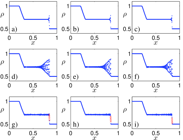
Figure 1: Density and velocity profile of the 1:2 isothermal shock tube simulation after $400$ time steps using (a) LBGK with polynomial quasiequilibria (20) [$\nu=3.3333\times 10^{-2}$]; (b) LBGK with entropic quasiequilibria (20) [$\nu=3.3333\times 10^{-2}$]; (c) ELBM (22) [$\nu=3.3333\times 10^{-2}$]; (d) LBGK with polynomial quasiequilibria (20) [$\nu=10^{-9}$]; (e) LBGK with entropic quasiequilibria (20) [$\nu=10^{-9}$]; (f) ELBM (22) [$\nu=10^{-9}$]; (g) LBGK with polynomial quasiequilibria and Ehrenfests’ steps (21) [$\nu=10^{-9}$, $(k,\delta)=(4,10^{-4})$]; (h) LBGK with entropic quasiequilibria and Ehrenfests’ steps (21) [$\nu=10^{-9}$, $(k,\delta)=(4,10^{-4})$]; (i) ELBM with Ehrenfests’ steps [$\nu=10^{-9}$, $(k,\delta)=(4,10^{-4})$]. Sites where Ehrenfests’ steps are employed are indicated by crosses.

We do not detect any advantage of using ELBM over LBGK with entropic quasiequilibria for this example. However, there appears to be some gain in employing entropic rather than polynomial quasiequilibria. We observe that the post-shock region for the unregularised LBGK simulations is more oscillatory when polynomial quasiequilibria are used. In Fig. 1 we have also included a panel with the simulation resulting from a much higher viscosity ($\nu=3.3333\times 10^{-2}$). Here, we observe no appreciable differences in the results of LBGK and ELBM.

4.2 Flow around a square-cylinder

Our second test is the $2$D unsteady flow around a square-cylinder. The realisation of LBGK that we use will employ a uniform $9$-speed square lattice with discrete velocities

$${\bf v}_{i}=\left\{\begin{aligned} &0,&\quad&\text{$i=0$,}\\ &\biggl{(}\cos\Bigl{(}(i-1)\frac{\pi}{2}\Bigr{)},\sin\Bigl{(}(i-1)\frac{\pi}{2}\Bigr{)}\biggr{)},&&\text{$i=1,2,3,4$,}\\ &\sqrt{2}\biggl{(}\cos\Bigl{(}(i-5)\frac{\pi}{2}+\frac{\pi}{4}\Bigr{)},\sin\Bigl{(}(i-5)\frac{\pi}{2}+\frac{\pi}{4}\Bigr{)}\biggr{)},&&\text{$i=5,6,7,8$.}\\ \end{aligned}\right.$$

The numbering $f_{0}$, $f_{1},\dotsc,f_{8}$ are for the static, east-, north-, west-, south-, northeast-, northwest-, southwest- and southeast-moving populations, respectively. Here, we select entropic quasiequilibria by maximising the entropy functional

$$S(f)=-\sum_{i}f_{i}\log{\Bigl{(}\frac{f_{i}}{W_{i}}\Bigr{)}},$$

subject to the constraints of conservation of mass and momentum [2]:

$$f_{i}^{*}=\rho W_{i}\prod_{j=1}^{2}\Bigl{(}2-\sqrt{1+3u_{j}^{2}}\Bigr{)}\Biggl{(}\frac{2u_{j}+\sqrt{1+3u_{j}^{2}}}{1-u_{j}}\Biggr{)}^{v_{i,j}}$$

Here, the lattice weights, $W_{i}$, are given lattice-specific constants: $W_{0}=4/9$, $W_{1,2,3,4}=1/9$ and $W_{5,6,7,8}=1/36$. As is usual, the macroscopic variables are given by the expressions

$$\rho:=\sum_{i}f_{i},\qquad\rho{\bf u}:=\sum_{i}{\bf v}_{i}f_{i}.$$

The computational set up for the flow is as follows. A square-cylinder of side length $L$, initially at rest, is emersed in a constant flow in a rectangular channel of length $30L$ and height $25L$. The cylinder is place on the centre line in the $y$-direction resulting in a blockage ratio of $4$%. The centre of the cylinder is placed at a distance $10.5L$ from the inlet. The free-stream fluid velocity is fixed at $(u_{\infty},v_{\infty})=(0.05,0)$ (in lattice units) for all simulations.

On the north and south channel walls a free-slip boundary condition is imposed (see, e.g., [25]). At the inlet, the inward pointing velocities are replaced with their quasiequilibrium values corresponding to the free-stream fluid velocity. At the outlet, the inward pointing velocities are replaced with their associated quasiequilibrium values corresponding to the velocity and density of the penultimate row of the lattice. Some care should to be taken with the boundary conditions on the cylinder, but for more information on these the reader may consult, e.g., [1, 3].

4.2.1 Strouhal–Reynolds relationship

As a test of the Ehrenfests’ regularisation, a series of simulations, all with characteristic length fixed at $L=20$, were conducted over a range of Reynolds numbers The parameter pair $(k,\delta)$, which control the Ehrenfests’ steps tolerances, are fixed at $(L/2,10^{-3})$.

We are interested in computing the Strouhal–Reynolds relationship. The Strouhal number $\mathrm{St}$ is a dimensionless measure of the vortex shedding frequency in the wake of one side of the cylinder:

$$\mathrm{St}=\frac{Lf_{\omega}}{u_{\infty}},$$

where $f_{\omega}$ is the shedding frequency.

For our computational set up, the vortex shedding frequency is computed using the following algorithmic technique. Firstly, the $x$-component of velocity is recorded during the simulation over $t_{\mathrm{max}}=1250L/u_{\infty}$ time steps. The monitoring points is positioned at coordinates $(4L,-2L)$ (assuming the origin is at the centre of the cylinder). Next, the dominant frequency is extracted from the final $25$% of the signal using the discrete Fourier transform. The monitoring point is purposefully placed sufficiently downstream and away from the centre line so that only the influence of one side of the cylinder is recorded.

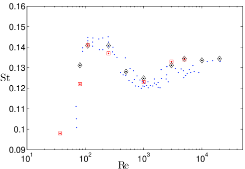
Figure 2: Variation of Strouhal number as a function of Reynolds. Dots are Okajima’s experimental data [23] (the data has been digitally extracted from the original paper). Diamonds are the Ehrenfests’ regularisation of LBGK and the squares are the ELBM simulation from [3].

The computed Strouhal–Reynolds relationship using the Ehrenfests’ regularisation of LBGK is shown in Fig. 2. The simulation compares well with Okajima’s data from wind tunnel and water tank experiment [23]. The present simulation extends previous LBM studies of this problem [3, 4] which have been able to quantitively captured the relationship up to $\mathrm{Re}\sim 1000$. Fig. 2 also shows the ELBM simulation results from [3]. Furthermore, the computational domain was fixed for all the present computations, with the smallest value of the kinematic viscosity attained being $\nu=5\times 10^{-5}$ at $\mathrm{Re}=20000$. It is worth mentioning that, for this characteristic length, LBGK exhibits numerical divergence at around $\mathrm{Re}=1000$. We estimate that, for the present set up, the computational domain would require at least $\sim 10^{7}$ lattice sites for the kinematic viscosity to be large enough for LBGK to converge at $\mathrm{Re}=20000$. This is compared with $\sim 10^{5}$ sites for the present simulation.

Appendix A Moments of the quasiequilibrium distribution

In this appendix we calculate the moments of the distribution $f^{*}$ so as to keep the presentation in the main body of the paper clean. All integrals are over the whole velocity space. Firstly, we have by definition

$$\int f^{*}\,\mathrm{d}{\bf v}=\rho,\qquad\int v_{i}f^{*}\,\mathrm{d}{\bf v}=\rho u_{i},\qquad\int{\bf v}^{2}f^{*}\,\mathrm{d}{\bf v}=2E=2P+\rho{\bf u}^{2}.$$

Next, we have

$$\int v_{i}v_{j}f^{*}\,\mathrm{d}{\bf v}=\int(v_{i}-u_{i})(v_{j}-u_{j})f^{*}\,\mathrm{d}{\bf v}+\rho u_{i}u_{j}.$$ (23)

Now, using the identity

$$\int\alpha\beta\mathrm{e}^{-(\alpha^{2}+\beta^{2})}\,\mathrm{d}\alpha\mathrm{d}\beta=0,$$

it follows by a change of variables that, for $i\neq j$,

$$\int(v_{j}-u_{j})(v_{i}-u_{i})f^{*}\,\mathrm{d}{\bf v}=0.$$

Further, it follows from the identity

$$\int\alpha^{2}\mathrm{e}^{-(\alpha^{2}+\beta^{2})}\,\mathrm{d}\alpha\mathrm{d}\beta=\int\beta^{2}\mathrm{e}^{-(\alpha^{2}+\beta^{2})}\,\mathrm{d}\alpha\mathrm{d}\beta$$

that

$$\begin{split}\int(v_{j}-u_{j})^{2}f^{*}\,\mathrm{d}{\bf v}&=\frac{1}{2}\int({\bf v}-{\bf u})^{2}f^{*}\,\mathrm{d}{\bf v}\\ &=\frac{1}{2}\int({\bf v}^{2}+{\bf u}^{2}-2v_{1}u_{1}-2v_{2}u_{2})f^{*}\,\mathrm{d}{\bf v}\\ &=\frac{1}{2}({2P}+\rho{\bf u}^{2}+\rho{\bf u}^{2}-2\rho u_{1}^{2}-2\rho u_{2}^{2})\\ &=P.\end{split}$$

Hence, from (23), we have

$$\int v_{i}v_{j}f^{*}\,\mathrm{d}{\bf v}=\delta_{i,j}{P}+\rho u_{i}u_{j}.$$ (24)

Finally, similar calculations provide us with

$$\int v_{\ell}v_{i}v_{j}f^{*}\,\mathrm{d}{\bf v}=(\delta_{i,j}u_{\ell}+\delta_{\ell,j}u_{i}+\delta_{\ell,i}u_{j}){P}+\rho u_{\ell}u_{i}u_{j}.$$ (25)

References

• [1] S. Ansumali and I. V. Karlin. Kinetic boundary conditions in the lattice Boltzmann method. Phys. Rev. E, 66(2):026311, 2002.
• [2] S. Ansumali S, I. V. Karlin, H.C. Ottinger, Minimal entropic kinetic models for hydrodynamics Europhys. Let. 63 (6): 798-804. 2003.
• [3] S. Ansumali, S. S. Chikatamarla, C. E. Frouzakis, and K. Boulouchos. Entropic lattice Boltzmann simulation of the flow past square-cylinder. Int. J. Mod. Phys. C, 15:435–445, 2004.
• [4] G. Baskar and V. Babu. Simulation of the unsteady flow around rectangular cylinders using the ISLB method. In 34th AIAA Fluid Dynamics Conference and Exhibit, pages AIAA–2004–2651, 2004.
• [5] P. L. Bhatnagar, E. P. Gross, and M. Krook. A model for collision processes in gases I. Small amplitude processes in charged and neutral one-component systems. Phys. Rev. 94(3):511–525, 1954.
• [6] R. A. Brownlee, A. N. Gorban, and J. Levesley. Stabilisation of the lattice-Boltzmann method using the Ehrenfests’ coarse-graining. cond-mat/0605359, 2006.
• [7] R. A. Brownlee, A. N. Gorban, and J. Levesley. Stabilisation of the lattice-Boltzmann method using the Ehrenfests’ coarse-graining. Phys. Rev. E, 74:037703, 2006.
• [8] R. A. Brownlee, A. N. Gorban, and J. Levesley, Stability and stabilization of the lattice Boltzmann method: Magic steps and salvation operations. cond-mat/0611444, 2006.
• [9] R. A. Brownlee, A. N. Gorban, and J. Levesley, Stability and stabilization of the lattice Boltzmann method. Phys. Rev. E, to appear.
• [10] H. Chen, S. Chen, W. Matthaeus, Recovery of the Navier–Stokes equation using a lattice–gas Boltzmann Method Phys. Rev. A 45 (1992), R5339–R5342.
• [11] R. W. Davis and E. F. Moore. A numerical study of vortex shedding from rectangles. J. Fluid Mech., 116:475–506, 1982.
• [12] P. Ehrenfest and T. Ehrenfest. The conceptual foundations of the statistical approach in mechanics. Dover Publications Inc., New York, 1990.
• [13] A. N. Gorban. Basic types of coarse-graining. In: A. N. Gorban, N. Kazantzis, I. G. Kevrekidis, H.-C. Öttinger, and C. Theodoropoulos, editors, Model Reduction and Coarse-Graining Approaches for Multiscale Phenomena, pages 117–176. Springer, Berlin-Heidelberg-New York, 2006. cond-mat/0602024.
• [14] A. Gorban, B. Kaganovich, S. Filippov, A. Keiko, V. Shamansky, I. Shirkalin, Thermodynamic Equilibria and Extrema: Analysis of Attainability Regions and Partial Equilibrium, Springer, Berlin, Heidelberg, New York, 2006 (in press).
• [15] A. N. Gorban and I. V. Karlin. Invariant manifolds for physical and chemical kinetics, volume 660 of Lect. Notes Phys. Springer, Berlin-Heidelberg-New York, 2005.
• [16] A. N. Gorban, I. V. Karlin, H. C. Öttinger, and L. L. Tatarinova. Ehrenfest’s argument extended to a formalism of nonequilibrium thermodynamics. Phys. Rev. E, 62:066124, 2001.
• [17] F. Higuera, S. Succi, and R. Benzi. Lattice gas – dynamics with enhanced collisions. Europhys. Lett., 9:345–349, 1989.
• [18] I. V. Karlin, S. Ansumali, C. E. Frouzakis, and S. S. Chikatamarla, Elements of the lattice Boltzmann method I: Linear advection equation. Commun. Comput. Phys., 1 (2006), 616–655.
• [19] I. V. Karlin, S. S. Chikatamarla and S. Ansumali. Elements of the lattice Boltzmann method II: Kinetics and hydrodynamics in one dimension. Commun. Comput. Phys., 2 (2007), 196–238.
• [20] I. V. Karlin, A. Ferrante, and H. C. Öttinger. Perfect entropy functions of the lattice Boltzmann method. Europhys. Lett., 47:182–188, 1999.
• [21] I. V. Karlin, A. N. Gorban, S. Succi, and V. Boffi. Maximum entropy principle for lattice kinetic equations. Phys. Rev. Lett., 81:6–9, 1998.
• [22] S. Kullback, Information theory and statistics, Wiley, New York, 1959.
• [23] A. Okajima. Strouhal numbers of rectangular cylinders. J. Fluid Mech., 123:379–398, 1982.
• [24] X. Shan and X. He Discretization of the velocity space in the solution of the Boltzmann equation Phys. Rev. Lett., 80:65–68, 1998.
• [25] S. Succi. The lattice Boltzmann equation for fluid dynamics and beyond. OUP, New York, 2001.
• [26] Y. H. Qian, D. d’Humieres, P. Lallemand, Lattice BGK models for Navier–Stokes equation, Europhys. Lett. 17, (1992), 479–484.
• [27] B. J. Vickery, Fluctuating lift and drag on a long cylinder of square cross-section in a smooth and in a turbulent stream. J. Fluid Mech., 25:481–494, 1966.
• [28] G. S. Yablonskii, V. I. Bykov, A. N. Gorban, and V. I. Elokhin, Kinetic Models of Catalytic Reactions (Series “Comprehensive Chemical Kinetics,” V.32, ed. by R. G. Compton), Elsevier, Amsterdam, 1991.
• [29] Y. B. Zeldovich, Proof of the Uniqueness of the Solution of the Equations of the Law of Mass Action, In: Selected Works of Yakov Borisovich Zeldovich, Vol. 1, J. P. Ostriker (Ed.), Princeton University Press, Princeton, USA, 1996, 144–148.