Dynamical heterogeneities and the breakdown
of the Stokes-Einstein and Stokes-Einstein-Debye relations
in simulated water

Abstract

We study the Stokes-Einstein (SE) and the Stokes-Einstein-Debye (SED) relations, $D_{t}=k_{B}T/6\pi\eta R$ and $D_{r}=k_{B}T/8\pi\eta R^{3}$ where $D_{t}$ and $D_{r}$ are translational and rotational diffusivity respectively, $T$ is the temperature, $\eta$ the viscosity, $k_{B}$ the Boltzmann constant and $R$ is the “molecular” radius, using molecular dynamics simulations of the extended simple point charge model of water. We find that both the SE and SED relations break down at low temperature. To explore the relationship between these breakdowns and dynamical heterogeneities (DH), we also calculate the SE and SED relations for subsets of the $7\%$ “fastest” and $7\%$ “slowest” molecules. We find that the SE and SED relations break down in both subsets, and that the breakdowns occur on all scales of mobility. Thus these breakdowns appear to be generalized phenomena, in contrast with the view where only the most mobile molecules are the origin of the breakdown of the SE and SED relations, embedded in an inactive background where these relations hold. At low temperature, the SE and SED relations in both subsets of molecules are replaced with “fractional” SE and SED relations, $D_{t}\sim(\tau/T)^{-\xi_{t}}$ and $D_{r}\sim(\tau/T)^{-\xi_{r}}$ where $\xi_{t}\approx 0.84<1$ and $\xi_{r}\approx 0.75<1$. We also find that there is a decoupling between rotational and translational motion, and that this decoupling occurs in both fastest and slowest subsets of molecules. We also find that when the decoupling increases, upon cooling, the probability of a molecule being classified as both translationally and rotationally fastest also increases. To study the effect of time scale for SE and SED breakdown and decoupling, we introduce a time-dependent version of the SE and SED relations, and a time-dependent function that measures the extent of decoupling. Our results suggest that both the decoupling and SE and SED breakdowns are originated at the time scale corresponding to the end of the cage regime, when diffusion starts. This is also the time scale when the DH are more relevant. Our work also demonstrates that selecting DH on the basis of translational or rotational motion more strongly biases the calculation of diffusion constants than other dynamical properties such as relaxation times.

I Introduction

At temperatures where liquids have a diffusion constant similar to that of ambient temperature water, the translational and rotational diffusion, $D_{t}$ and $D_{r}$ respectively, are well described by the Stokes-Einstein (SE) relation einstein

$$D_{t}=\frac{k_{B}T}{6\pi\eta R}$$ (1)

and Stokes-Einstein-Debye (SED) relation debye

$$D_{r}=\frac{k_{B}T}{8\pi\eta R^{3}},$$ (2)

where $T$ is the temperature, $\eta$ the viscosity, $k_{B}$ the Boltzmann constant and $R$ is the “molecular” radius. These equations are derived by a combination of classical hydrodynamics (Stokes’ Law) and simple kinetic theory (e.g, the Einstein relation) soft-matter . Recently the limits of the SE and SED relations have been an active field of experimental andreozzi ; rossler ; swallen ; cicedi ; chen-sed ; chenbo , theoretical stillhod ; lepo ; ngai ; kimkeyes ; franosch ; tarjus ; coniglio ; saltz and computational lepo2 ; netzbarb ; matsui ; heuer ; bps ; chand ; kumdoug ; zetter ; bordat ; kumarpnas ; kbbsps ; jung research. The general consensus is that the SE and SED relations hold for low-molecular-weight liquids for $T\gtrsim 1.5T_{g}$, where $T_{g}$ is the glass transition temperature. For $T\lesssim 1.5T_{g}$, deviations from either one or both of the SE and SED relations are observed. Experimentally it is found that the SE relation holds for many liquids in their stable and weakly supercooled regimes, but when the liquid is deeply supercooled it overestimates $D_{t}$ relative to $\eta$ by as much as two or three orders of magnitude, a phenomenon usually referred to as the “breakdown” of the SE relation. The situation for the SED relation is more complex. Some experimental studies found agreement with the predicted values of the SED relation even for deeply supercooled liquids cicedi ; ediger-rev ; sillescu-rev , while others claim also a breakdown of the SED relation to the same extent as for the SE relation chang ; doss ; steffen ; fischer ; rossler . The failure of these relations provides a clear indication of a fundamental change in the dynamics and relaxation of the system. Indeed, the changing dynamics of the liquid as it approaches the glass transition is well documented, but not yet fully understood angell ; nico-rev ; ediger_glass ; pablo .

There is a large body of evidence weeks ; bohmer ; tracht ; deschenes ; deschenesJPC that, upon cooling, the liquid does not become a glass in a spatially homogeneous fashion richert ; sillescu-rev ; ediger-rev ; glotzer-rev ; kivFLD ; ngai-PRE . Instead the system is characterized by the appearance of regions in which the structural relaxation time can differ by orders of magnitude from the average over the entire system tamm . The liquid is characterized by the presence of “dynamical heterogeneities” (DH), in which the motion of atoms or molecules is highly spatially correlated. The presence of these DH is argued to give rise to the breakdown of the SE relation stillhod ; tarjus . Since the derivation of the Einstein relation assumes uncorrelated motion of particles, it is reasonable that the emergence of correlations could result in a failure of the SE relation. The aim of the present work is to assess the validity of the SE and SED relations in the SPC/E model of water, and consider to what extent the DH contribute to the SE and SED breakdown.

Computer simulations have been particularly useful for studying DH (e.g., see Refs. hh ; melcuk ; pan ; shell ; kobdonati ; nicoPRL ) since simulations have direct access to the details of the molecular motion. For water, the existence of regions of enhanced or reduced mobility has also been identified nicoPRL ; matharoo . In particular, Ref. nicoPRL identifies the clusters of molecules with greater translational (or center of mass) mobility with the hypothesized “cooperatively rearranging regions” of the Adam-Gibbs approach AG ; steve-wolynes .

Most computer simulation studies on DH describe these heterogeneities based on the particle or molecule translational degrees of freedom. We will refer to these DH as translational heterogeneities (TH). For water, it is also necessary to consider the rotational degrees of freedom of the molecule. Recently, some computer simulation studies on molecular systems described the DH based on the molecular rotational degrees of freedom lepo2 ; KKS ; andreozzi ; matsui ; kimkeyes1 ; kimlikeyes ; first . We will refer to these DH as rotational heterogeneities (RH). For the case of a molecular model of water, RH were studied first and it was found that RH and TH are spatially correlated. This work extends those results. We find support for the idea that TH are connected to the failure of the SE relation, and further that RH have a similar effect on SED relation. Additionally, we find that the breakdown of these relations is accompanied by the decoupling of the translational and rotational motion.

This work is organized as follows. In the next section we describe the water model and simulation details. In Sec. III and Sec. IV we test the validity of the SE and SED relations and their connection with the presence of DH, respectively. The decoupling between rotational and translation motion is studied in Sec. V. In Sec. VI we explore the role of time scale in the breakdown of the SE and SED relations and decoupling of rotational and translational motion. We summarize our results in Sec. VII. We have placed some technical aspects of the work in appendices to facilitate the flow of our results.

II Model and Simulation Method

We perform molecular dynamics (MD) simulations of the SPC/E model of water spce . This model assumes a rigid geometry for the water molecule, with three interaction sites corresponding to the centers of the hydrogen (H) and oxygen (O) atoms. Each hydrogen has a charge $q_{H}=0.4238~{}e$, and the oxygen charge is $q_{O}=-2.0~{}q_{H}$, where $e$ is the magnitude of the electron charge. The OH distance is $1.0$ Å and the HOH angle is $109.47^{\circ}$, corresponding to the tetrahedral angle. In addition to the Coulombic interactions, a Lennard-Jones interaction is present between oxygen atoms of two different molecules; the Lennard-Jones parameters are $\sigma=3.166$ Å and $\epsilon=0.6502$ kJ/mol. We use a cutoff distance of $2.5\sigma=7.915$ Å  for the pair interactions and the reaction field technique stein is used to treat the long range Coulombic interactions.

We perform simulations in the constant particle number, $N$, volume, $V$, and temperature $NVT$ ensemble with $N=1728$ water molecules and fixed density $\rho=1.0$ g/cm³. The values of the simulated temperature are $T=210$, $220$, $230$, $240$, $250$, $260$, $270$, $280$, $290$, $300$, $310$, $330$ and $350$ K. We use the Berendsen method berend to keep the temperature constant. We use periodic boundary conditions and a simulation time step of $1$ fs. To ensure that simulations attain a steady-state equilibrium, we perform equilibration simulations for at least the duration specified by Ref. francislong . After these equilibration runs we continue with production runs of equal duration during which we store the coordinates of all atoms for data analysis. To improve the statistics of our results, we have performed $5$ independent simulations for each $T$. Ref. francislong provides further details of the simulation protocol.

III Breakdown of the SE and SED relations

To assess the validity of the SE and SED relations we consider a simple rearrangement of Eqs. (1) and (2), i.e. we define the SE ratio

$$R_{\rm SE}\equiv\frac{D_{t}\eta}{T}$$ (3)

and the SED ratio

$$R_{\rm SED}\equiv\frac{D_{r}\eta}{T}.$$ (4)

Both $R_{\rm SE}$ and $R_{\rm SED}$ will be temperature-independent if the SE and SED relations are valid.

To evaluate $R_{\rm SE}$ and $R_{\rm SED}$, we must first calculate the appropriate diffusion constants. Following normal procedure, we define

$$D_{t}\equiv\lim_{\Delta t\to\infty}\frac{1}{6\Delta t}\langle r^{2}(\Delta t)\rangle.$$ (5)

where $\langle r^{2}(\Delta t)\rangle$ is the translational mean square displacement (MSD) of the oxygen atoms

$$\langle r^{2}(\Delta t)\rangle\equiv\frac{1}{N}\sum_{i=0}^{N}|\vec{r}_{i}(t^{\prime})-\vec{r}_{i}(t)|^{2}.$$ (6)

Here, $\vec{r}_{i}(t)$ and $\vec{r}_{i}(t^{\prime})$ are the positions of the oxygen atom of molecule i at time $t$ and $t^{\prime}$ respectively, and $\Delta t=t^{\prime}-t$. Analogously, we define the rotational diffusion coefficient

$$D_{r}\equiv\lim_{\Delta t\to\infty}\frac{1}{4\Delta t}\langle\varphi^{2}(\Delta t)\rangle,$$ (7)

where $\langle\varphi^{2}(\Delta t)\rangle$ is the rotational mean square displacement (RMSD) for the vector rotational displacement $\vec{\varphi}_{i}(\Delta t)$. Special care must be taken to calculate $\langle\varphi^{2}(\Delta t)\rangle$ so that it is unbounded. A detailed discussion of this procedure is provided in Appendix A.

We also need the viscosity $\eta$ to evaluate $R_{\rm SE}$ and $R_{\rm SED}$. Unfortunately, accurate calculation of $\eta$ is computationally challenging. A frequently employed approximation exploits the fact that $\eta$ is proportional to the shear stress relaxation time, $\tau_{s}$, via the infinite frequency shear modulus, $G_{\infty}$, which is nearly $T$-independent mcdonal . Additionally, we expect that $\tau_{s}$ (a “collective property”) should be nearly proportional to other collective relaxation times, such as the relaxation time $\tau$ defined from the coherent intermediate scattering function, $F(q,\Delta t)$, where $q$ is the wave vector. Therefore, we substitute $\eta$ by $\tau$, which should only affect the value and units of the constants in the $R_{\rm SE}$ and $R_{\rm SED}$. For the purposes of our calculations, we define $\tau$ by fitting $F(q,\Delta t)$ at long times with a “stretched” exponential

$$F(q,\Delta t)\sim\exp{[-(\Delta t/\tau)^{\beta}]},$$ (8)

where $0<\beta<1$, and we focus on the $q$ value corresponding to the first peak in the static structure factor $S(q)$.

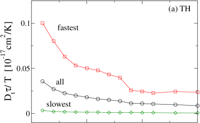
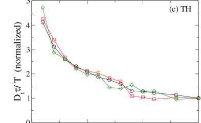
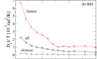
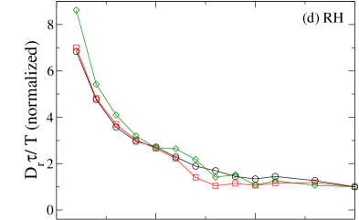
Figure 1: (a) SE ratio, $D_{t}\tau/T$, for the $7\%$ most translationally mobile molecules (“fastest”), for the $7\%$ least translationally mobile molecules (“slowest”), and for the entire system (all). There is a breakdown of the SE relation (constant SE ratio) at low temperatures in both the fastest and slowest subsets, as well as for the entire system. (b) SED ratio, $D_{r}\tau/T$, for the $7\%$ most rotationally mobile molecules, for the $7\%$ least rotationally mobile molecules, and for the entire system (all). Similar to (a), there is a breakdown of the SED relation (constant SED ratio). (c) and (d) Normalization of the curves in (a) and (b), respectively, by the corresponding quantities at $T=350$ K. The collapse of these curves demonstrates that the relative deviations from the SE and SED relations are approximately the same for the corresponding mobility subsets.

Now that we have the necessary quantities, we show $R_{\rm SE}$ and $R_{\rm SED}$ in Fig. 1(a) and Fig. 1(b) with the curves labelled with “all”. Both quantities deviate at low $T$ from the corresponding constant values reached at high temperature indicating a breakdown of both the SE and SED relations.

Whether there is a breakdown of the SED relation in experiments is not clear. While some experiments measuring dipole relaxation times show that the SED relation holds down to the glass transition ediger-rev ; sillescu-rev , other experiments ludemann show that the SED relation fails for low $T$. Our simulations are in agreement with the breakdown of the SED ratio observed in, e.g., Ref. bps . Figures 1(a) and 1(b) also show $R_{\rm SE}$ and $R_{\rm SED}$ for different subsets of molecules to examine the role played by DH. This is discussed in the following Section.

IV Role of dynamical heterogeneities

IV.1 Identifying mobility subsets

Many theoretical approaches (e.g. stillhod ; tarjus ) attempt to explain the breakdown of SE and/or SED in terms of DH. To this end, we must first describe the procedure used to select molecules whose motion (or lack thereof) is spatially correlated. A variety of approaches have been used to probe the phenomenon of DH. Here we use one of the most common techniques: partitioning a system into mobility groups based on their rotational or translational maximum displacement.

For the TH, we define the translational mobility, $\mu_{i}$, of a molecule $i$ at a given time $t_{0}$ and for an observation time $\Delta t$, as the maximum displacement over the time interval $[t_{0},t_{0}+\Delta t]$ of its oxygen atom

$$\mu_{i}(t_{0},\Delta t)\equiv\max\{|\vec{r}_{i}(t+t_{0})-\vec{r}_{i}(t_{0})|\,,\,t_{0}\leq t\leq t_{0}+\Delta t\}.$$ (9)

For the RH, following first , we define a rotational mobility that is analogous to the translational case. In analogy with Eq. (9), we define the rotational mobility at time $t_{0}$ with an observation time $\Delta t$ as

$$\psi_{i}(t_{0},\Delta t)\equiv\max\{|\vec{\varphi}_{i}(t+t_{0})-\vec{\varphi}_{i}(t_{0})|\,,\,t_{0}\leq t\leq t_{0}+\Delta t\}\,.$$ (10)

We identify the subsets of rotationally and translationally “fastest” molecules as the $7\%$ of the molecules with largest $\psi_{i}$ and $\mu_{i}$, respectively. Analogously, we identify the subsets of rotationally and translationally “slowest” molecules as the $7\%$ of the molecules with smallest $\psi_{i}$ and $\mu_{i}$, respectively. The choice of $7\%$ is made to have a direct comparison with the analysis of Ref. nicoPRL ; first , but the qualitative details of our work are unaffected by modest changes in this percentage. In the following, we will refer to these subsets of molecules as TH and RH, fastest and slowest, depending on whether we consider the top or the bottom of the distribution of mobilities. We will see that comparing the fastest and the slowest molecules will reveal new features of DH.

IV.2 SE and SED relations for fastest and slowest molecules

Having identified subsets of highly mobile or immobile molecules, we can calculate the ratios $R_{\rm SE}$ and $R_{\rm SED}$ by limiting the evaluation of $D_{t}$, $D_{r}$ and $\tau$ to these subsets. This is relatively straightforward for the diffusion constants, since they depend only on single molecule averages. For $\tau$, the situation is more complex since $F(q,\Delta t)$ includes cross-correlations between molecules. Hence we specialize the definition of $F(q,\Delta t)$ for the TH and RH subsets by introducing a definition that captures the cross-correlation within subsets and between a subset and rest of the system. We call this function $F_{\rm subset}(q,\Delta t)$, which we discuss in detail in Appendix B.

We show the value of $R_{\rm SE}$ and $R_{\rm SED}$ in Fig. 1(a) and 1(b) for the cases when only the fastest and slowest subsets of molecules are considered. Like the total system average, both the SE and SED ratios for the subsets deviate at low $T$ from the corresponding constant value reached at high temperature. Therefore, we observe that the breakdowns of both the SE and SED relations occur not only in the subset of the fastest molecules, but also in the slowest. We have also confirmed a breakdown in intermediate subsets.

The most mobile subset of molecules has a consistently greater value of $D_{t}\tau/T$ and $D_{r}\tau/T$ than the rest of the system, while the ratios for the least mobile subsets are always smaller. This is a result of the fact that the means by which we select the different subsets most strongly affects the diffusion constant (see Appendix B), and hence the differences in the SE and SED ratios between the full system and the subsets are dominated by the diffusion constant, rather than by the relaxation time.

In order to compare the relative deviations of these curves from the SE and SED predictions, we normalize $R_{\rm SE}$ and $R_{\rm SED}$ by their respective high temperature values [Fig. 1(c) and 1(d)]. We observe that there is a collapse of all the curves; thus, we conclude that both the most and least mobile molecules contribute in the same fashion to the breakdown of SE and SED. Moreover, this result supports the scenario that the deviation from the SE and SED relations cannot be attributed to only one particular subset of fastest/slowest molecules, but to all scales of translational and rotational mobility. We have confirmed this by looking at subsets of intermediate mobility (not shown). Therefore, we interpret our results as a sign of a generalized breakdown in the system under study, in contrast to a picture where only the most mobile molecules are the origin of the breakdown of SE and SED, embedded in an inactive background where the SE and SED equations hold (see e.g. cicedi ). These results are consistent with the results of Ref. bps , who arrived at the same conclusion via a different analysis.

IV.3 Fractional SE and SED relations

When the SE and SED relations fail, it is frequently observed that they can be replaced by fractional functional forms poll ; cicedi96 ; swallen ; boc ; vor ; chang ; andreozzi2 ; andreozzi ; biel

$$D_{t}\sim\left({\tau\over T}\right)^{-\xi_{t}},\quad D_{r}\sim\left({\tau\over T}\right)^{-\xi_{r}}$$ (11)

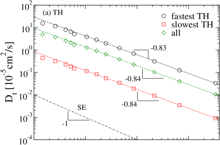
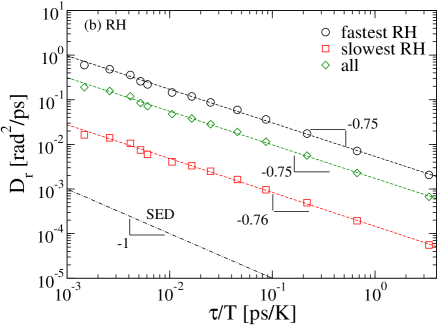
Figure 2: (a) Power law fits of translational diffusivity $D_{t}$ as functions of $\tau/T$, $D_{t}\sim(\tau/T)^{-\xi_{t}}$, for the eight values of temperature $T=210$ $\dots$ $280$ K (but not for the remaining values $T=290$ $\dots$ $350$ K), for fastest TH, slowest TH, and all molecules. We estimate $\xi_{t}\approx 0.84$. The dot-dashed line represents the normal SE behavior ($\xi_{t}=1$). Consistently with the results of Fig. 1, the deviation of these three curves from the SE behavior is almost identical as reflected in the values of these fractional exponents. (b) Power law fits of rotational diffusivity, $D_{r}$, as functions of $\tau/T$, $D_{r}\sim(\tau/T)^{-\xi_{r}}$, of simulations in the same temperature range of (a) for fastest RH, slowest RH, and all molecules. We estimate $\xi_{r}\approx 0.75$. The dot-dashed line represents the normal SED behavior ($\xi_{r}=1$). Also for RH, a fractional law is found with the same exponents for the three families considered, and, noticeably, the deviation from the normal case ($\xi_{r}=1$), is stronger for $D_{r}$ than for $D_{t}$, since $\xi_{r}<\xi_{t}$.

with $\xi_{t}<1$ and $\xi_{r}<1$. Hence we test to what degree Eqs. (11) hold for our system. In Fig. 2 we show a parametric plot of diffusivity versus $\tau/T$ for the entire system, and for the fastest and slowest molecules composing the TH and RH. The results at low temperature are well fit with the fractional form of SE and SED relations. From Fig. 2, $\xi_{t}$ for TH is $0.83,0.84,0.84$ for fastest, slowest, and all, respectively, so all TH have approximately the same exponent. Similarly, for RH we find that $\xi_{r}$ is $0.75,0.76,0.75$ for fastest, slowest, and all, respectively.

Reference bps found a stronger form of this fractional relation. Specifically, Ref. bps examined an “ensemble” of systems of the ST2 water model at the same $T$, which by statistical variation have fluctuations in the SE and SED ratios. Nonetheless, all systems collapsed to the same master curve when plotted in the parametric form shown in Fig. 2, meaning that the systems dominated by mobile or immobile molecules collapse to the same curve. While Ref. bps employed a very different method (small systems followed for shorter times), the conclusion of our Fig. 2 is the same: a generalized deviation from SE and SED. However, Fig. 2 clearly shows that we do not find a general collapse in our present calculation. To understand why, we return to the fact that the method by which we define mobility affects much more strongly the diffusion constants than the coherent relaxation time, $\tau$. As a result, it is impossible to have the data for the mobile and immobile subsets to collapse to a single master curve. To observe the same collapse, presumably one needs a more “neutral” method for selecting the mobile particles—that is one that does not explicitly bias toward a specific property. Unfortunately, such an approach is not obvious. However, we reproduced the ensemble approach of Ref. bps , by splitting each of our 5 simulations into 3 trajectories. We obtain reasonable fluctuations that allow us to test and confirm (not shown) the observation of collapse of Ref. bps . Hence, the phenomenon of homogeneous breakdown of SE and SED appears to be robust for the different water models.

V Decoupling of Translational and Rotational Motions

The SE and SED relations also imply a coupling between rotational and translational motion. Specifically, Eqs. (1) and (2) imply that the ratio

$$\frac{D_{r}}{D_{t}}=\frac{3}{4R^{2}}$$ (12)

should remain constant as a function of temperature. Since we have already seen that the SE and SED ratios are not obeyed, it is likely that the ratio $D_{r}/D_{t}$ is also violated ber . However, it is also possible that $D_{r}/D_{t}$ remains constant if both $D_{r}$ and $D_{t}$ deviate from their expected behavior in the same way.

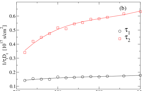
Figure 3: (a) The ratio of rotational and translational diffusivities $D_{r}/D_{t}$ as a function of temperature. As temperature decreases, this ratio increases indicating a decoupling between rotation and translational motion. The deviation of $D_{r}$ is stronger than that of $D_{t}$. The line is a guide for the eye. (b) Same as (a) where the rotational diffusivity, $D_{r}$, is replaced by the inverse of the rotational relaxation time, $\tau_{\ell}$ with $\ell=1,2$, as usually done in experiments. An opposite decoupling is observed in (a) and (b). The lines are guides for the eye.

Figure 3(a) shows $D_{r}/D_{t}$ as a function of temperature. As $T$ decreases, we observe that $D_{r}/D_{t}$ increases, which implies that the breakdown of the SED relation is more pronounced than that of the SE relation.

Experiments generally do not examine the behavior of $D_{r}/D_{t}$ since $D_{r}$ is not accessible. Instead, $D_{r}$ is usually replaced by $(\tau_{\ell})^{-1}$ with $\ell=2$ netzbarb . Here, $\tau_{\ell}$ is the relaxation time of the rotational correlation function

$$C_{\ell}(\Delta t)=\langle P_{\ell}(\cos[\hat{p}(t)\cdot\hat{p}(t+\Delta t)])\rangle,$$ (13)

where $P_{\ell}(x)$ is the Legendre polynomial of order $\ell$, and $\hat{p}(t)$ is defined in Appendix A. Figure 3(b) shows $(\tau_{\ell})^{-1}/D_{t}$ for $\ell=1,2$. We observe that $(\tau_{\ell})^{-1}/D_{t}$ also shows a decoupling between rotational and translational motion. However, while $D_{r}/D_{t}$ increases upon cooling, $(\tau_{\ell})^{-1}/D_{t}$ decreases upon cooling. MD simulations using an ortho-terphenyl (OTP) model OTP and the ST2 water model bps also find an opposite decoupling of the SE and SED relations depending on whether $D_{r}$ or $\tau_{2}$ is used. In the simulations of OTP, it was shown that the inverse relation between $D_{r}$ and $\tau_{2}$ fails due to the caging of the rotational motion; this caging results in intermittent large rotations that are not accounted for by the Debye approximation.

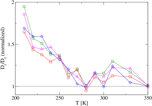
Figure 4: The ratio of rotational and translational diffusivities, $D_{r}$ and $D_{t}$ respectively, for the following choices of subsets: $D_{r}$ for fastest TH divided by $D_{t}$ for fastest TH ($\lozenge$), $D_{r}$ for slowest TH divided by $D_{t}$ for slowest TH ($\vartriangle$), $D_{r}$ for fastest RH divided by $D_{t}$ for fastest RH ($\bigcirc$), $D_{r}$ for slowest RH divided by $D_{t}$ for slowest RH ($\square$). The values were normalized by the $T=350$ K values for every curve. The fact that for these four cases $D_{r}/D_{t}$ deviates from unity (dashed line) to approximately the same degree indicates that the decoupling occurs across all four cases.

Similar to the analysis of the breakdown of the SE and SED ratios, we can test whether DH play a strong role in the decoupling by examining the ratio $D_{r}/D_{t}$ for the different mobility subsets. This is slightly complicated by the fact that we can choose mixed mobility subsets when calculating the ratio. Figure 4 shows that the ratio $D_{r}/D_{t}$ for all choices of mobility subsets approximately coincide when scaled by the high temperature behavior of $D_{r}/D_{t}$. This indicates that (like the breakdown of the SE and SED relations) the decoupling is uniform across the subsets of mobility.

VI Time scales for breakdown and decoupling

VI.1 Time dependent SE and SED relations

The SE and SED relations depend on $D$ and $\eta$, which are defined only in the asymptotic limit of infinite time. In contrast, the time scale on which DH exist is finite, and generally shorter that the time scale on which the system becomes diffusive. As a result, making the connection between DH and the breakdown of SE and SED expressions is difficult. To address this complication, we incorporate a time dependence in the SE and SED relations, so that we can evaluate these relations at the time scale of the DH. This point has been neglected so far in the literature. To define time-dependent versions of the SE and SED ratios, we first define time-dependent diffusivities

$$D_{t}(\Delta t)\equiv\frac{\langle r^{2}(\Delta t)\rangle}{6\Delta t}\,,\,\,D_{r}(\Delta t)\equiv\frac{\langle\varphi^{2}(\Delta t)\rangle}{4\Delta t},$$ (14)

and we also define time-dependent relaxation times

$$\tau(\Delta t)\equiv\int_{t}^{t+\Delta t}F(q,t^{\prime})dt^{\prime}\,.$$ (15)

Note that $D_{t}(\Delta t)\to D_{t}$ and $D_{r}(\Delta t)\to D_{r}$ in the limit $\Delta t\to\infty$. The definition of $\tau(\Delta t)$ requires some explanation: $\tau(\Delta t)$ is the time integral of the intermediate scattering function, and $\tau(\Delta t)$ will be proportional to the standard relaxation time $\tau$ [Eq. (8)] in the limit $\Delta t\to\infty$. There is a constant of proportionality resulting from the stretched exponential form note-1 . When, instead, a DH is considered, $F_{\rm subset}(q,\Delta t)$ [see Eq. (21)] is used in the computation of $\tau(\Delta t)$. We choose these definitions since, in the limit $\Delta t\to\infty$, they converge or are proportional to the corresponding time-independent definitions. We will use these time-dependent quantities to examine time-dependent generalizations of $R_{\rm SE}$ [Eq. (3)] and $R_{\rm SED}$ [Eq. (4)].

VI.2 Breakdown time scale

Analyzing the time-dependent ratio $D(\Delta t)\tau(\Delta t)/T$ (for either rotational or translational motion) allows one to verify quantitatively the role of the time scale in the SE/SED ratios. To contrast the behavior of $D(\Delta t)\tau(\Delta t)/T$ with the average over the entire system, we define the time dependent “breakdown” ratios as follows:

$$b_{\rm DH}(\Delta t)\equiv\frac{\left(D(\Delta t)\tau(\Delta t)/T\right)_{\rm DH}}{\left(D(\Delta t)\tau(\Delta t)/T\right)_{\rm all}}$$ (16)

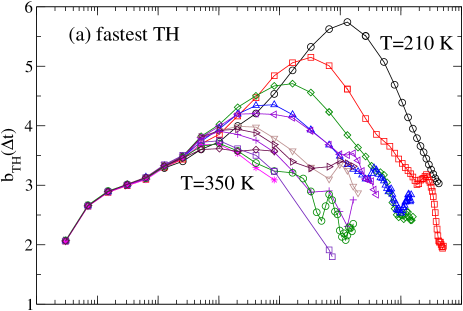
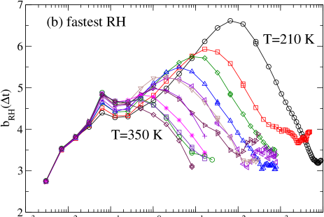
Figure 5: (a) Time-dependent extension, $b_{\rm TH}(\Delta t)$, of the SE relation for the fastest TH at different $T$. For the sake of clarity the curve corresponding to $T=290$ K was removed. (b) Time-dependent extension, $b_{\rm RH}(\Delta t)$, of the SED relation for the fastest RH at different $T$. For the sake of clarity the curve corresponding to $T=290$ K was removed. In both (a) and (b), the maxima occur at the time scales corresponding to the end of the cage regime, when DH are more pronounced. These maxima increase upon cooling, as the DH become more pronounced.

where DH refers to TH or RH. If the DH are related to the breakdown of the SE and SED relations, then one would expect that: (i) the $b_{\rm TH}$ and $b_{\rm RH}$ ratios will show the largest deviations from the system average behavior at the time scale when DH are most pronounced, i.e. approximately at a time which we denote as $t^{*}$, at which the non-Gaussian parameter is a maximum (see Appendix C). (ii) The lower the $T$, the larger the peak of $b_{\rm DH}$ is (in agreement with the fact that the DH are more pronounced as $T$ decreases). Figure 5(a) for TH and Fig. 5(b) for RH, show the behavior of $b_{\rm DH}(\Delta t)$ for the fastest subset of molecules, for different temperatures. Both expectations (i) and (ii) agree with Fig. 5.

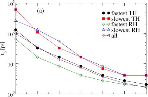
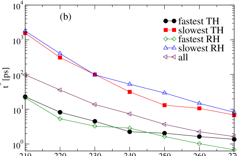
Figure 6: Temperature dependence of (a) $t_{b}$, the time at which the time-dependent extensions of the SE and SED relations, $b_{\rm DH}$, have maxima, and (b) $t^{*}$, the time at which the non-Gaussian parameter, $\alpha_{2}(\Delta t)$, reaches a maximum. $t^{*}$ indicates the time scale corresponding to the end of the cage regime. We show the results when considering molecules belonging to TH, RH, and also for the entire system.

From Fig. 5 we can extract the time $t_{b}$ when $b_{\rm DH}(\Delta t)$ is a maximum. Figure 6(a) shows $t_{b}$ for each of the four subsets: TH fastest/slowest and RH fastest/slowest. If DH play a significant role in the breakdown of the SE and SED relations, we would expect that the maximum contribution to the deviation from the SE and SED relations, occurring at $t_{b}$, coincides roughly with the “classical” measure of the characteristic time of DH, $t^{*}$. Comparison of Fig. 6(a) and Fig. 6(b) for $T<280$ K shows that $t^{*}$ is slightly larger than $t_{b}$ for the slowest DH, while is shorter than $t_{b}$ for fastest DH. Nonetheless, $t_{b}$ and $t^{*}$ are approximately the same, and so the largest contribution to the SE/SED ratio is on the time scale when DH are most pronounced. This provides direct evidence for the idea that the appearance of DH is accompanied by the failure of the SE and SED ratios.

VI.3 Decoupling time scales

We next directly probe the relation between DH and the decoupling of $D_{r}$ and $D_{t}$. As discussed above, the time scale at which the DH are observable is much smaller than the time scale at which the system is considered diffusive. Therefore, in analogy to the previous section, we incorporate a time scale in the $D_{r}/D_{t}$ ratio so that we can compare the decoupling between rotation and translation at the time scale of the DH. To this end we introduce the ratio

$$d_{\rm DH}(\Delta t)\equiv{(D_{r}(\Delta t)/D_{t}(\Delta t))_{\rm DH}\over(D_{r}(\Delta t)/D_{t}(\Delta t))_{\rm all}},$$ (17)

where DH refers to TH or RH.

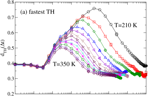
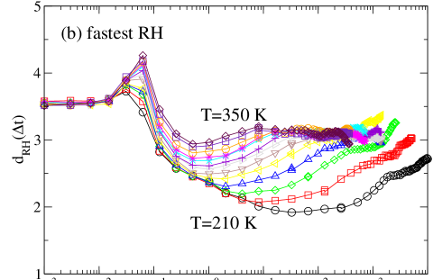
Figure 7: (a) Temporal behavior of the ratio of the time-dependent rotational diffusivity and translational diffusivity for fastest TH, normalized by the average over the entire system. We show all the simulated temperatures. (b) Temporal behavior of the ratio of the time-dependent rotational diffusivity and translational diffusivity for fastest RH, normalized by the average over the entire system. We show all the simulated temperatures. The figure shows that the decoupling of rotation from translation is increasingly more pronounced as $T$ decreases and is a maximum (a) or minimum (b) on the time scale of the DH.

Figure 7(a) shows the results for $d_{TH}(\Delta t)$ for the fastest subsets of molecules. For short times, $d_{TH}(\Delta t)$ does not depend on time and temperature, since in this initial temporal regime the dynamics at all temperatures is ballistic, i.e., both $\langle\varphi^{2}(\Delta t)\rangle$ and $\langle r^{2}(\Delta t)\rangle$ are approximately linear with $(\Delta t)^{2}$. At intermediate times $d_{TH}(\Delta t)$ develops a distinct maximum which increases in magnitude and shifts to larger observation times as $T$ is reduced. The maximum occurs at the time scale where the fastest molecules of the TH and RH “break their cages” and enter the corresponding diffusive regimes, see Fig. 6(b). Therefore, the results of Fig. 7(a) also suggest that the decoupling between rotational and translational motion is largest at approximately the same time scale at which the DH are most pronounced. We note from Fig. 7(a) that $d_{TH}(\Delta t)<1$, indicating that the decoupling of rotational and translational motion observed in the fastest subsets of TH is smaller than that from the average over the entire system. As we focus in slower subsets of TH for the same $T$, we observe that the maximum in $d_{TH}(\Delta t)$ decreases at any given $T$.

Figure 7(b) shows $d_{RH}(\Delta t)$ for the fastest subsets of molecules. Similar to the behavior of $d_{TH}(\Delta t)$, at short times $d_{RH}(\Delta t)$ does not depend on time nor temperature; molecules move ballistically in this regime. The maxima in $d_{RH}(\Delta t)$ at $\Delta t\approx 0.1$ ps for all temperatures are a consequence of the librational molecular motion, enhanced in this case because we are selecting the fastest subset of RH. At intermediate times, we observe a broad minimum in $d_{RH}(\Delta t)$ centered at $\Delta t\approx t^{*}$; this minimum becomes deeper and shifts to later times upon cooling, suggesting that the decoupling in the fastest subset of RH is largest at approximately the same time scale at which the DH are more pronounced. The fact that $d_{TH}(\Delta t)$ shows a maximum at approximately $t^{*}$, while $d_{RH}(\Delta t)$ shows a minimum at $t^{*}$ is because fastest subsets of RH tend to enhance the rotational motion with respect to the translational motion, while the opposite situation occurs for the fastest subsets of TH. We note from Fig. 7(b) that $d_{RH}(\Delta t)>1$, indicating that the decoupling of rotational and translational motion observed in the fastest subsets of RH is larger than that found in the average over the entire system.

In short, the behavior of $d_{TH}(\Delta t)$ and $d_{RH}(\Delta t)$ indicates that the emergence of DH is correlated to the rotation/translation decoupling, just as it does for the breakdown of the SE and SED relations.

VII Summary

In this work, we tested in the SPC/E model for water (i) the validity of the SE and SED equations, (ii) the decoupling of rotational and translational motion, and (iii) the relation of (i) and (ii) to DH. We found that at low temperatures there is a breakdown of both the SE and SED relations and that these relations can be replaced by fractional functional forms. The SE breakdown is observed in every scale of translational mobility. Similarly, the SED breakdown is observed in every scale of rotational mobility. Thus our results support the view of a generalized breakdown, instead of a view where only the most mobile molecules are the origin of the breakdown of the SE and SED relations, embedded in an inactive background where these relations hold.

We also found that, upon cooling, there is a decoupling of translational and rotational motion. This decoupling is also observed in all scales of rotational and translational mobilities. In agreement with MD simulations of an OTP model OTP , we find that an opposite decoupling is observed depending on whether one uses the rotational diffusivity, $D_{r}$, or the rotational relaxation time, $\tau_{2}$. In the first case, rotational motion is enhanced upon cooling with respect to the translational motion, while the opposite situation holds when choosing $\tau_{2}$. This is particularly relevant for experiments, where typically only $\tau_{2}$ is accessible.

We also found that as the decoupling of $D_{r}/D_{t}$ increases, the number of molecules belonging simultaneously to both RH and TH also increases. This is counter-intuitive since a stronger decoupling would suggest less overlapping of TH and RH. Therefore we conclude that the decoupling of $D_{r}/D_{t}$ is significant even at the single molecule level.

We also explored the role of time scales in the breakdown of the SE and SED relations and decoupling. To do this we introduced time dependent versions of the SE and SED expressions. Our results suggest that both the decoupling and SE and SED breakdowns are originated at the time scale corresponding to the end of the cage regime, when diffusion starts. This is also the time scale at which the DH are more relevant.

Our work also demonstrates that selecting DH on the basis of translational or rotational displacement more strongly biases the calculation of diffusion constants than the other dynamical properties. If appropriate care is taken, this should not be problematic, but it does make apparent that an alternative approach to identify DH would be valuable. This is especially true when contrasting behavior of diffusion constants and relaxation times, as is the case for the SE and SED relations.

VIII Acknowledgments

We would like to thank S.R. Becker, P.G. Debenedetti, J. Luo, T.G. Lombardo, P.H. Poole, and S. Sastry for useful discussions. We thank the NSF for support under grant number CHE-06-16489.

Appendix A Evaluation of the Rotational Mean Square Displacement

To calculate $D_{r}$ [Eq. (7)] we consider the behavior of the normalized polarization vector $\hat{p}_{i}(t)$ for molecule $i$ (defined as the normalized vector from the center of mass of the water molecule to the midpoint of the line joining the two hydrogens). The molecular rotation will cause a rotation of $\hat{p}_{i}(t)$. A naive definition of angular displacement as $\hat{p}_{i}(t)-\hat{p}_{i}(0)$ would be insensitive to full molecular rotations, since it would result in a bounded quantity. Following Ref. KKS , we avoid this complication by defining the vector rotational displacement in the time interval $[t,t+\Delta t]$ as

$$\vec{\varphi}_{i}(\Delta t)\equiv\int_{t}^{t+\Delta t}\Delta\vec{\varphi}_{i}(t^{\prime})dt^{\prime},$$ (18)

where $\Delta\vec{\varphi}_{i}(t^{\prime})$ is a vector with direction given by $\hat{p}_{i}(t^{\prime})\times\hat{p}_{i}(t^{\prime}+dt^{\prime})$ and with magnitude given by $|\Delta\vec{\varphi}_{i}(t^{\prime})|\equiv\cos^{-1}\left(\,\hat{p}_{i}(t^{\prime})\cdot\hat{p}_{i}(t^{\prime}+dt^{\prime})\right)$, i.e., the angle spanned by $\hat{p}_{i}$ in the time interval $[t^{\prime},t^{\prime}+dt^{\prime}]$. Thus, the vector $\vec{\varphi}_{i}(\Delta t)$ allows us to define a trajectory in a $3\text{D}$ space representing the rotational motion of molecule $i$, analogous to the trajectory defined by $\vec{r}_{i}(\Delta t)$ for the translational case. We define, in analogy to MSD, a rotational mean square displacement (RMSD) first ; lepo2 ; KKS

$$\langle\varphi^{2}(\Delta t)\rangle\equiv\frac{1}{N}\sum_{i=0}^{N}|\vec{\varphi}_{i}(t+\Delta t)-\vec{\varphi}_{i}(t)|^{2}.$$ (19)

Using this form, we define $D_{r}$ as given by Eq. (7), analogous to the definition of $D_{t}$. We have verified that there is no qualitative difference, in the results of the present work, when the polarization vector is replaced by the other two principal directions of the water molecule.

Appendix B Correlation functions for Dynamical heterogeneities

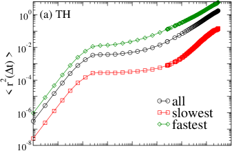
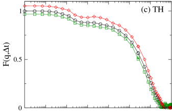
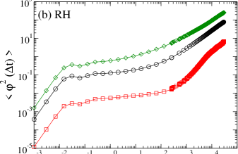
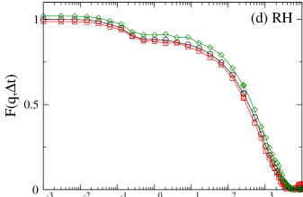
Figure 8: Example of time correlation functions limited to subsets of DH. (a) MSD and (b) RMSD at $T=210$ K for the fastest and slowest TH and RH respectively, as well as for the entire system. Intermediate scattering function, $F(q,\Delta t)$, at $T=210$ K for (c) the fastest and slowest TH, and entire system and (d) the fastest and slowest RH and the entire system.

We introduce a MSD, $\langle r^{2}(\Delta t)\rangle$, for the fastest and slowest subsets of molecules by limiting the sum in the Eq. (6) to the molecules in the corresponding subset. The different MSDs at $T=210$ K are shown in Fig. 8(a). We note that since the most and least mobile $7\%$ of the molecules will generally vary as a function of time, the molecules used to calculate $\langle r^{2}(\Delta t)\rangle$ will change with time; in other words, when a molecule ceases being part of a DH, it is no longer considered in the computation of the MSD and the focus is shifted to the new subset of molecules belonging to the DH considered. Analyzing the $\langle r^{2}(\Delta t)\rangle$ for the collection of subsets from most mobile to least mobile has the advantage that the mean of $\langle r^{2}(\Delta t)\rangle$ over the subsets converges to the MSD for the full system. In a similar fashion the RMSD, $\langle\varphi^{2}(\Delta t)\rangle$, is calculated also for the fastest and slowest rotationally mobile molecules [Fig. 8(b)].

To complement the single particle dynamics determined by $\langle r^{2}(\Delta t)\rangle$ and $\langle\varphi^{2}(\Delta t)\rangle$, we also evaluate the coherent intermediate scattering function

$$F(q,\Delta t)\equiv\frac{1}{N\,S(q)}\sum_{j=1}^{N}e^{-iqr_{j}(t+\Delta t)}\sum_{k=1}^{N}e^{iqr_{k}(t)},$$ (20)

where $S(q)$ is the structure factor. $F(q,\Delta t)$ reflects two-particle temporal correlations instead of single-particle correlations (as in the case of the MSD). The normalization factors ensure that $F(q,0)=1$. In analogy to our analysis of $\langle r^{2}(\Delta t)\rangle$, we would like to evaluate the contribution to $F(q,\Delta t)$ made by subsets of molecules. Naively, one might think this can be simply done by limiting the sums in Eq. (20) to solely those molecules within the subset. However, taking the mean over the subsets of such a quantity will not recover the complete $F(q,\Delta t)$, since there will be no information on the cross-correlations between the subsets. In order to include these correlations and define a function that, when averaged over subsets, will return $F(q,\Delta t)$ (as is the case for MSD and RMSD), we simply limit one of the two sums to the subset, while the other sum still extends over all molecules. Mathematically, we define

$$F_{\rm subset}(q,\Delta t)\equiv\frac{1}{N_{\rm subset}\,S(q)}\sum_{j=1}^{N}e^{-iqr_{j}(t+\Delta t)}\sum_{k\in subset}e^{iqr_{k}(t)}.$$ (21)

Note that one must make the choice whether to limit the sum to the subset at time $t$ or $t+\Delta t$; we have found that in practice there is little, if any, qualitative difference in this choice. Thus we measure the correlations between the subset of molecules at time $t$ with all molecules at time $t+\Delta t$. Additionally, $F_{\rm subset}(q,0)$ is not necessarily $1$; forcing this normalization would not satisfy the desired condition that the mean over subsets returns the average over all molecules. In all cases, we evaluate $F_{\rm subset}(q,\Delta t)$ at $q=18$ nm^-1, the value of the transferred momentum at the first maximum of the structure factor where the relaxation is slowest (except for the $q\rightarrow 0$ limit). Figure 8(c) and 8(d) show $F(q,\Delta t)$ for all molecules, and for the fastest and the slowest TH and RH.

At this point, it is important to compare the behavior of $\langle r^{2}(\Delta t)\rangle$ and $\langle\varphi^{2}(\Delta t)\rangle$ with that of $F(q,\Delta t)$ for the TH and RH subsets. Since we define mobility on the basis of displacement, the behavior of $\langle r^{2}(\Delta t)\rangle$ and $\langle\varphi^{2}(\Delta t)\rangle$ for the subsets are much more strongly affected than $F_{\rm subset}(q,\Delta t)$ for the subsets. Additionally, $F_{\rm subset}(q,\Delta t)$ includes cross-correlations both within and between subsets that a single particle definition of mobility does not include. More specifically, the data in Fig. 8 at $T=210$ K show that there is roughly two orders of magnitude difference between $\langle r^{2}(\Delta t)\rangle$ for the most and least mobile molecules (and similar difference for $\langle\varphi^{2}(\Delta t)\rangle$). We also find that there is roughly also two orders of magnitude difference between the most and least mobile molecules for $D_{t}$ and $D_{r}$. For higher $T$, the difference is less pronounced. When we examine the relaxation of $F(q,\Delta t)$ for the most and least mobile subsets, we find only a difference of a factor of $\approx$ 2 between the time scales for relaxation. Therefore — not surprisingly — selecting mobility based on single particle displacement results in a much stronger effect on diffusion than it does for collective relaxation phenomena. This fact is important for the comparison between this work and a previous work bps .

Appendix C Characteristic time of Dynamical heterogeneities

Since we analyze the DH both in the context of translational and rotational motions, it is natural to ask at what time scale the TH and RH are more pronounced and to what degree the TH and RH subsets overlap each other. References nicoPRL and first show that the fastest subsets of TH and RH form clusters, and that these clusters are larger at approximately the time $t^{*}$ corresponding to the onset of the diffusive regime, as indicated by $\langle r^{2}(\Delta t)\rangle$ and $\langle\varphi^{2}(\Delta t)\rangle$ respectively. Normally $t^{*}$ for the translational case is defined as the maximum in the non-Gaussian parameter rahman

$$\alpha_{2}(\Delta t)\equiv\frac{3<r^{4}(\Delta t)>}{5<r^{2}(\Delta t)>}-1\,,$$ (22)

where $\langle r^{4}(\Delta t)\rangle$ and $\langle r^{2}(\Delta t)\rangle$ are the fourth and second moment of the displacement distribution, respectively (the last is also the MSD). $\alpha_{2}(\Delta t)$ is known to be identically zero for a Gaussian distribution, and thus it signals when the dynamics does not generate such a Gaussian distribution of displacements. In the present study, we use either translational, $\vec{r}_{i}(\Delta t)$, or rotational, $\vec{\varphi}_{i}(\Delta t)$, displacement for TH and RH, respectively, when computing $\alpha_{2}(\Delta t)$. Figure 6(b) shows $t^{*}$ as a function of $T$ defined for the fastest and slowest subsets of both the TH and RH. We also include the corresponding values of $t^{*}$ for the entire system. Figure 6(b) shows that there is no qualitative difference in shape of the curve of $t^{*}(T)$ for the different subsets considered and the entire system.

Since the values of $t^{*}$ for TH and RH are similar, we expect that there is some coupling between TH and RH. Previously, Chen et al. chengallo found that there is coupling between translational and rotational motion at large transferred momentum $q$. The maximum correlation occurs at the cage relaxation time, $t^{*}$, for large values of $q$. Ref. first found a spatial correlation between RH and TH. Along similar lines, we examine the overlap between these subsets. Figure 9 shows the overlap between the fastest subset of molecules belonging to TH and RH, as a function of $\Delta t$ and $T$. Specifically, we count the number of fastest molecules belonging simultaneously to TH and RH as a function of observation time $\Delta t$. Similar to Fig. 9 in Ref. chengallo , the strength of this coupling reaches its maximum at the cage relaxation times, but these times are consistently shorter than those reported in chengallo ; this is likely to be due to the fact that we consider fastest TH and fastest RH in this calculation, while Ref. chengallo considers all the molecules of the system. Figure 9 indicates that, at the lowest temperature simulated, about $45\%$ of the molecules comprising the fastest subset of TH coincide with the ones in the fastest subset of RH.

Figure 9: Fraction of molecules belonging simultaneously to both fastest TH and fastest RH versus observation time $\Delta t$, at different temperatures. This overlap of fastest TH and fastest RH is maximum at the end of the cage regime and increases upon cooling. It is almost $45\%$ at the lowest $T$.

References

- (1) A. Einstein, Investigations on the Theory of the Brownian Motion (Dover, New York, 1956).
- (2) P. Debye, Polar Molecules (Dover, New York, 1929).
- (3) R.A.L. Jones, Soft Condensed Matter (Oxford Univ. Press, Oxford, 2002).
- (4) L. Andreozzi, M. Bagnoli, M. Faetti and M. Giordano, J. Non-Cryst Sol. 303, 262 (2002).
- (5) E. Rössler, Phys. Rev. Lett. 65, 1595 (1990).
- (6) S.F. Swallen, P.A. Bonvallet, R.J. McMahon and M.D. Ediger, Phys. Rev. Lett. 90, 015901 (2003).
- (7) M.T. Cicerone, F.R. Blackburn and M.D. Ediger, J. Chem. Phys. 102, 471 (1995); F.R. Blackburn, C.-Y. Wang and M.D. Ediger, J. Phys. Chem. 100, 18249 (1996)
- (8) S.-H. Chen, F. Mallamace, C.-Y. Mou, M. Broccio, C. Corsaro, A. Faraone and L. Liu, Proc. Natl. Acad. Sci. USA 103, 12974 (2006).
- (9) B. Chen, E.E. Sigmund and W.P. Halperin, Phys. Rev. Lett. 96, 145502 (2006).
- (10) F.H. Stillinger and J.A.Hodgdon, Phys. Rev. E 50, 2064 (1994).
- (11) J.F. Douglas and D. Leporini, J. Non-Cryst Sol. 235-237, 137 (1998).
- (12) K.L. Ngai, J. Phys. Chem. B 103, 10684 (1999).
- (13) J. Kim and T. Keyes, J. Phys. Chem. B 109, 21445 (2005).
- (14) T. Franosch, M. Fuchs, W. Götze, M.R. Mayr and A.P. Singh, Phys. Rev. E 56, 5659 (1997).
- (15) G. Tarjus and D. Kivelson, J. Chem. Phys. 103, 3071 (1995).
- (16) M. Nicodemi and A. Coniglio, Phys. Rev. E 57, R39 (1998).
- (17) K.S. Schweizer and E.J. Saltzman, J. Phys. Chem. B 108, 19729 (2004).
- (18) C. De Michele and D. Leporini, Phys. Rev. E 63, 036702 (2001).
- (19) P.A. Netz, M.C. Barbosa and H.E. Stanley, J. Mol. Liq. 101, 159 (2002).
- (20) G. Matsui and S. Kojima, Phys. Lett. A 293, 156 (2002).
- (21) J. Qian, R. Hentschke and A. Heuer, J. Chem. Phys. 110, 4514 (1999).
- (22) S.R. Becker, P.H. Poole and F.W. Starr, Phys. Rev. Lett. 97, 055901 (2006).
- (23) L. Berthier, D. Chandler and J.P. Garrahan, Europhys. Lett. 69, 320 (2005).
- (24) S.K. Kumar, G. Szamel and J.F. Douglas, J. Chem. Phys. 124, 214501 (2006).
- (25) M. Dzugutov, S.I. Simdyankin and F.H.M. Zetterling, Phys. Rev. Lett. 89, 195701 (2002).
- (26) P. Bordat, F. Affouard, M. Descamps and F. Müller-Plathe, J. Phys.: Condens. Matter 15, 5397 (2003).
- (27) P. Kumar, Proc. Natl. Acad. Sci. USA 103, 12955 (2006).
- (28) P. Kumar, S.V. Buldyrev, S.R. Becker, F.W. Starr, P.H. Poole and H. E. Stanley, Proc. Natl. Acad. Sci. USA 104, 9575 (2007).
- (29) Y.-J. Jung, J.P. Garrahan and D. Chandler, Phys. Rev. E 69, 061205 (2004).
- (30) M.D. Ediger, Annu. Rev. Phys. Chem. 51, 99 (2000).
- (31) H. Sillescu, J. Non-Cryst. Sol. 243, 81 (1999).
- (32) I. Chang and H. Sillescu, J. Phys. Chem. B 101, 8794 (1997).
- (33) A. Döß, G. Hinze, B. Schiener, J. Hemberger, and R. Böhmer, J. Chem. Phys. 107, 1740 (1997).
- (34) W. Steffen, A. Patkowski, G. Meier, and E.W. Fischer, J. Chem. Phys. 96, 4171 (1992).
- (35) E.W. Fischer, E. Donth, and W. Steffen, Phys. Rev. Lett. 68, 2344 (1992).
- (36) C. A. Angell, Science 267, 1924 (1995).
- (37) T. Loerting and N. Giovambattista, J. Phys.: Condens. Matter 18, R919 (2006).
- (38) M. D. Ediger, C. A. Angell and S. R. Nagel, J. Phys. Chem. 100, 13200 (1996).
- (39) P. G. Debenedetti, Metastable Liquids (Princeton Univ. Press, Princeton, 1996).
- (40) E.R. Weeks, J.C. Crocker, A.C. Levitt, A. Schofield and D.A. Weitz, Science 287, 627 (2000).
- (41) R. Böhmer, R.V. Chamberlin, G. Diezemann, B. Geil, A. Heuer, G. Hinze, S.C. Kuebler, R. Richert, B. Schiener, H. Sillescu, H.W. Spiess, U. Tracht and M. Wilhelm, J. Non-Cryst Sol. 235-237, 1 (1998).
- (42) U. Tracht, M. Wilhelm, A. Heuer, H. Feng, K. Schmidt-Rohr and H.W. Spiess, Phys. Rev. Lett. 81, 2727 (1998).
- (43) L.A. Deschenes and D.A. Vanden Bout, Science 292, 255 (2001).
- (44) L.A. Deschenes and D.A. Vanden Bout, J. Phys. Chem. B 106, 11438 (2002).
- (45) R. Richert, J. Phys.: Condens. Matter 14, R703 (2002).
- (46) S.C. Glotzer, J. Non-Cryst. Sol. 274, 342 (2000).
- (47) S. A. Kivelson, X.-C. Zeng, D. Kivelson, C. M. Knobler and T. Fischer, J. Chem. Phys. 101, 2391 (1994).
- (48) K. Y. Tsang and K. K. Ngai, Phys. Rev. E 54, R3067 (1996).
- (49) First suggested by G. Tammann, Der Glasszustand (Leopold Voss, Leipzig, 1933).
- (50) M. M. Hurley and P. Harrowell, Phys. Rev. E 52, 1694 (1995); D. N. Perera and P. Harrowell, J. Chem. Phys. 111, 5441 (1999); Phys. Rev. Lett. 81, 120 (1998); A. Widmer-Cooper, P. Harrowell and H. Fynewever, Phys. Rev. Lett. 93, 135701 (2004); A. Widmer-Cooper and P. Harrowell, Phys. Rev. Lett. 96, 185701 (2006).
- (51) A. I. Mel’cuk, R. A. Ramos, H. Gould, W. Klein and R. D. Mountain, Phys. Rev. Lett. 75, 2522 (1995).
- (52) A.C. Pan, J.P. Garrahan and D. Chandler, Phys. Rev. E 72, 041106 (2005).
- (53) M.S. Shell, P.G. Debenedetti and F.H. Stillinger, J.Phys.: Condens. Matter 17, S4035 (2005).
- (54) W. Kob, C. Donati, S. J. Plimpton, P. H. Poole and S. C. Glotzer, Phys. Rev. Lett. 79, 2827 (1997); C. Donati, J. F. Douglas, W. Kob, S. J. Plimpton, P. H. Poole and S. C. Glotzer, Phys. Rev. Lett. 80, 2338 (1998).
- (55) N. Giovambattista, S.V. Buldyrev, F.W. Starr and H.E. Stanley, Phys. Rev. Lett. 90, 085506 (2003).
- (56) G. S. Matharoo, M. S. Gulam Razul and P. H. Poole, Phys. Rev. E 74, 050502(R) (2006).
- (57) G. Adam and J.H. Gibbs, J. Chem. Phys. 43, 139 (1965).
- (58) J.D. Stevenson, J. Schmalian and P.G. Wolynes, Nature Physics 2, 268 (2006).
- (59) S. Kammerer, W. Kob and R. Schilling, Phys. Rev. E 56, 5450 (1997).
- (60) J. Kim and T. Keyes, J. Chem. Phys. 121, 4237 (2004).
- (61) J. Kim, W.-X. Li and T. Keyes, Phys. Rev. E 67, 021506 (2003).
- (62) M.G. Mazza, N. Giovambattista, F.W. Starr and H.E. Stanley, Phys. Rev. Lett. 96, 057803 (2006).
- (63) H.J.C. Berendsen, J.R. Grigera and T.P. Stroatsma, J. Phys. Chem. 91, 6269 (1987).
- (64) O. Steinhauser, Mol. Phys. 45, 335 (1982).
- (65) H.J.C. Berendsen, J.P.M. Postma, W.F. van Gunsteren, A. DiNola and J. R. Haak, J. Chem. Phys. 81, 3684 (1984).
- (66) F.W. Starr, F. Sciortino and H.E. Stanley, Phys. Rev. E 60, 6757 (1999).
- (67) J.P. Hansen and I.R. McDonald, Theory of Simple liquids (Academic Press, 2006)
- (68) E.W. Lang, D. Girlich, H.-D. Lüdemann, L. Piculell and D. Müller, J. Chem. Phys. 93, 4796 (1990).
- (69) G. L. Pollack, Phys. Rev. A 23, 2660 (1981); G. L. Pollack and J. J. Enyeart, Phys. Rev. A 31, 980 (1985).
- (70) M.T. Cicerone and M.D. Ediger, J. Chem. Phys. 104, 7210 (1996).
- (71) L. Bocquet, J. P. Hensen, and J. Piasecki, J. Stat. Phys. 76, 527 (1994).
- (72) A. Voronel, E. Veliyulin, V.Sh. Machavariani, A. Kisliuk and D. Quitmann, Phys. Rev. Lett. 80, 2630 (1998).
- (73) L. Andreozzi, A. Di Schino, M. Giordano and D. Leporini, Europhys. Lett. 38, 669 (1997).
- (74) S. Hensel-Bielowka, T. Psurek, J. Ziolo and M. Paluch, Phys. Rev. E 63, 062301 (2001); T. Psurek, S. Hensel-Bielowka, J. Ziolo and M. Paluch, J. Chem. Phys. 116, 9882 (2002).
- (75) L. Berthier, Phys. Rev. E 69, 020201 (2004).
- (76) T.G. Lombardo, P.G. Debenedetti, and F.H. Stillinger, J. Chem. Phys. 125, 174507 (2006).
- (77) Assuming a Kohlrausch form for the intermediate scattering function, , the integral will yield , where is the Euler Gamma function.
- (78) A. Rahman, Phys. Rev. 136, A405 (1964).
- (79) See, for a discussion on the same question from the point of view of the intermediate scattering function, S.-H. Chen, P. Gallo, F. Sciortino, and P. Tartaglia, Phys. Rev. E 56, 4231 (1997).