Cassini UVIS Observations of the Io Plasma Torus.
IV. Modeling Temporal and Azimuthal Variability

Abstract

In this fourth paper in a series, we present a model of the remarkable temporal and azimuthal variability of the Io plasma torus observed during the Cassini encounter with Jupiter. Over a period of three months, the Cassini Ultraviolet Imaging Spectrograph (UVIS) observed a dramatic variation in the average torus composition. Superimposed on this long-term variation, is a 10.07-hour periodicity caused by an azimuthal variation in plasma composition subcorotating relative to System III longitude. Quite surprisingly, the amplitude of the azimuthal variation appears to be modulated at the beat frequency between the System III period and the observed 10.07-hour period. Previously, we have successfully modeled the months-long compositional change by supposing a factor of three increase in the amount of material supplied to Io’s extended neutral clouds. Here, we extend our torus chemistry model to include an azimuthal dimension. We postulate the existence of two azimuthal variations in the number of super-thermal electrons in the torus: a primary variation that subcorotates with a period of 10.07 hours and a secondary variation that remains fixed in System III longitude. Using these two hot electron variations, our model can reproduce the observed temporal and azimuthal variations observed by Cassini UVIS.

1 Introduction

During the Cassini spacecraft’s flyby of Jupiter (October 2000 through March 2001) the Ultraviolet Imaging Spectrograph (UVIS) made extensive observations of the Io plasma torus. The sensitivity, bandpass, resolution, and imaging capabilities of UVIS (Esposito et al., 2004) coupled with the temporal coverage of the observations make this a particularly rich dataset. Analysis and modeling of these observations has led to remarkable new insights into the behavior of the Io torus. In this paper we present the results of our efforts to model the temporal and azimuthal variability of the Io plasma torus observed by UVIS and discussed by Steffl et al. (2006). To put this effort into proper context, here we recapitulate the prior analysis and modeling of the Cassini UVIS observations.

Information about the UVIS Io torus dataset, including examples of the observing geometry, images of the raw and processed data, and descriptions of the data reduction and calibration techniques used was presented in paper I (Steffl et al., 2004a). The analysis of a small subset of UVIS Io torus observations obtained in January 2001, shortly after the Cassini spacecraft’s closest approach to Jupiter, was presented in Paper II (Steffl et al., 2004b). Using the CHIANTI atomic physics database (Dere et al., 1997; Young et al., 2003), they derived the composition and electron temperature of torus plasma as a function of radial distance from Jupiter. The torus composition presented in Paper II differs significantly from that derived from observations made in the Voyager era (Bagenal, 1994), with less oxygen and a lower electron temperature. The CHIANTI-based spectral model of the Io torus was used to analyze UVIS data obtained during a 45-day period on the Cassini spacecraft’s approach to Jupiter. Significant temporal and azimuthal variations in torus composition were found, which were presented in paper III (Steffl et al., 2006).

To understand the processes governing the Io plasma torus and their changes between the Voyager and Cassini epochs Delamere and Bagenal (2003) (hereafter referred to as DB03) developed a physical chemistry model of the Io torus which builds on previous modeling work by Barbosa et al. (1983), Shemansky (1988), Barbosa (1994), Schreier et al. (1998), and Lichtenberg et al. (2001). The DB03 model, from which the azimuthal models discussed below are directly descended, is a “0-d” or one-box model that calculates the flow of mass and energy through one cubic centimeter of torus plasma placed at a radial distance of 6 R_J. The effects of electron impact ionization, recombination (both radiative and dielectronic), charge exchange reactions, parameterized radial transport, Coulomb collisions between species, and radiative energy losses on the torus plasma are all included.

New mass is supplied to the torus in the form of neutral oxygen and sulfur atoms which eventually become ions through either electron impact ionization or charge exchange reactions. Conversely, mass is lost from the model when an ion becomes neutralized through charge exchange or recombination or through outward radial transport. The rotation speed of plasma in the Io torus ($\sim$75 km/s at 6 $R_{J}$) significantly exceeds Jupiter’s escape velocity. When torus ions becomes neutralized, the resulting atom is no longer constrained by Jupiter’s magnetic field and is quickly lost from the Io torus, eventually forming an extended nebula hundreds of Jovian radii in size (Mendillo et al., 2004). Torus plasma is also convected radially outwards by the interchange motions of magnetic flux tubes (Richardson and Siscoe, 1981; Siscoe and Summers, 1981). However, the details of convective radial transport are beyond the scope of the DB03 model; instead, the lifetime of torus plasma against radial transport is specified by an input parameter, $\tau_{0}$.

Energy is supplied to the torus via the “pickup energy” imparted to new ions as they are accelerated from Keplerian orbital velocities to near co-rotational with the magnetic field. As noted by Shemansky (1988), Smith et al. (1988), and others, pickup energy alone cannot supply the torus with enough energy to maintain roughly 10¹² W of UV radiation, a thermal electron temperature of $\sim$5 eV, and an average ionization state of $\sim$1.5, as are observed: an additional source of energy is required. It is now widely accepted that this additional energy is provided by a small population of super-thermal electrons. This is supported by detections of a high-energy component of the torus electron distribution function by both the Voyager (Scudder et al., 1981; Sittler and Strobel, 1987) and Galileo (Frank and Paterson, 2000) plasma instruments. In addition, analysis of Ulysses URAP observations showed the electron distribution function in the Io plasma torus resembles a kappa distribution (Meyer-Vernet et al., 1995).

In the torus model of DB03, the electron distribution function is simplified as the sum of two Maxwellian populations: a thermal population near the canonical 5 eV and a small (roughly 0.2% of the total electron density), hot population with temperature between 50–100 eV, consistent with Sittler and Strobel (1987). The temperature of the hot population is held constant at a value specified by the input parameter, $T_{e,hot}$. Since the hot electron population rapidly couples to the thermal electron population via Coulomb collisions (with a characteristic cooling time on the order of 30 minutes), maintaining a constant hot electron temperature requires the hot population be continuously resupplied with energy. For the plasma conditions observed by UVIS during the Cassini epoch, DB03 found the hot electron source was responsible for up to 60% (10¹² W) of the total energy input to the torus.

The energy for these hot electrons must ultimately be derived from Jupiter’s rotation, but the particular details of the heating mechanism remain poorly understood. Barbosa (1985) suggested that the hot electrons may be heated by lower hybrid waves generated during the thermalization of the pickup ion ring beam distribution. However, if Io’s extended neutral clouds are highly peaked near Io (Smyth and Marconi, 2003; Burger and Johnson, 2004; Smyth and Marconi, 2005), this mechanism will produce a 13-hour periodicity (the synodic period between Io and System III) which should be detectable in the Cassini UVIS observations. No such 13-hour periodicity was seen, suggesting that ring beam thermalization is not the dominant production mechanism. Thorne et al. (1997) reported rapid (100 km/s) inward motion of hot tenuous plasma during a flux tube interchange event. Such rapid motion could supply the Io torus with electrons that have been heated in the outer torus/middle magnetosphere. Alternatively, we propose that the hot electrons are produced locally throughout the torus during small-scale flux tube interchange events. These interchange events likely generate the field-aligned electron beams detected by the Galileo PLS (Frank and Paterson, 2000) in the shear region between inward and outward moving flux tubes.

An estimate of the total power available to the torus from these beams of field-aligned electrons can be made using the following equation:

$$P_{beam}=\Phi Tf\pi(r_{2}^{2}-r_{1}^{2})$$ (1)

where $\Phi$ is the flux of electrons in the field-aligned beams, $T$ is the average electron energy, $f$ is the fraction of the torus in which the beams occur, and $r_{1}$ and $r_{2}$ are radial distance of the inner and outer edges of the torus. From Frank and Paterson (2000), $\Phi\approx 10^{8}$ cm^-2 s^-1, $T\approx 500$ eV (ranging between 100 eV and a few keV), and $f\approx 0.1$. Assuming a torus that extends from 6.0 to 7.5 R_J, yields a total power input of a few 10¹² W, consistent with what is required by DB03.

While a discussion of the origin of these beams is beyond the scope of this paper, we note that a plausible heating mechanism is the propagation of inertial Alfvén waves out of the plasma torus, as was first discussed by Crary (1997) for the Io flux tube. We note that the energy spectrum (100 eV to few keV) of the beams reported by Frank and Paterson (2000) is consistent with electron acceleration to roughly the Alfvén velocity just outside of the torus. For additional discussion of acceleration by inertial Alfvén waves see Su et al. (2006) and Swift (2006).

1.1 Temporal variability during the Cassini era

Analysis of the Cassini UVIS observations of the Io torus showed significant changes in the composition of torus plasma between October 2000 and January 2001 (Steffl et al., 2006). During this period, the average mixing ratio (ion density divided by electron density) of S II in the torus declined by a factor of 2 during this period, with a corresponding factor of 2 increase in the mixing ratio of S IV. Observations by the Galileo Dust Detector System (DDS) showed a dramatic increase, by over three orders of magnitude, in the emission rate of Iogenic dust immediately prior to the UVIS observations (Krüger et al., 2003). The enhanced dust emissions began in July 2000, peaked in September 2000, and returned to pre-event levels by December 2000. Presumably, this increase (the largest, by an order of magnitude, observed by the Galileo DDS over a seven-year period) was in response to some major volcanic event on Io, possibly the eruption of Tvashtar Catena that deposited a Pele-like ring of red material 1200 km in diameter on Io’s surface between February 2000 and December 2000 (Geissler et al., 2004). A 400 km-high plume over this region was observed by the Cassini Imaging Science Subsystem in December 2000 (Porco et al., 2003).

These observations led Delamere et al. (2004) to propose that an increase in the amount of material supplied to the Io neutral clouds might be responsible for the compositional changes seen by Cassini UVIS. Their model included a Gaussian increase in the neutral source rate with an amplitude of 3.5 and a width of 22.5 days. As the supply of neutrals increased, the densities in the model torus rapidly increased to unrealistic levels, unless they were accompanied by a corresponding decrease in the radial transport timescale, $\tau$. Such an inverse relationship is expected if the radial transport of plasma is driven by flux tube interchange (Southwood and Kivelson, 1989; Brown and Bouchez, 1997; Pontius et al., 1998). Since, the exact functional form of the inverse relationship is dependent on the details of radial convective transport, which remain poorly understood, a variety of inverse relations were tested and a relation of $\tau\propto\mathcal{S}_{n}^{-1}$ was adopted. In this work, we extend the model of Delamere et al. (2004) to include an azimuthal dimension.

1.2 Azimuthal variability during the Cassini era

Superimposed on the long-term temporal variation in torus composition, UVIS observed a persistent azimuthal, i.e., longitudinal, asymmetry in plasma composition, electron temperature, and equatorial electron column density (Steffl et al., 2006). This nearly-sinusoidal azimuthal variation can be clearly seen in Fig. 1. The azimuthal variations of S II, S III, and electron column density mixing ratios are all approximately in phase with each other and are approximately 180^∘ out of phase with the variations of the mixing ratios of S IV and O II and the torus equatorial electron temperature.

Over short timescales ($\lesssim$50 hours), the observed azimuthal variability in the Io plasma torus is well described by a simple sinusoidal curve with a period equal to the 9.925-hour System III rotation period. However, the observed phase of the sinusoidal variation slowly drifts to greater System III longitudes, at a rate of 12.5^∘/day. This effect is clearly seen in the upper panel of Fig. 2. The rate of the phase increase implies that the compositional variations observed by UVIS rotate Jupiter with a period of 10.07 hours, 1.5% longer than the System III rotation period, yet 1.3% shorter than the previously observed “System IV” period Sandel and Dessler (1988); Brown (1995). Careful analysis of the UVIS observations using Lomb-Scargle periodograms (Lomb, 1976; Scargle, 1982; Horne and Baliunas, 1986) confirmed strong torus periodicity with a period of 10.07 hours (see Fig 7) and a secondary periodicity with a period close to the System III period of 9.925 hours.

Numerous ground-based observations have established that plasma in the Io torus lags rigid co-rotation with Jupiter’s magnetic field (Brown, 1983; Roesler et al., 1984; Brown, 1994a; Thomas et al., 2001). It is therefore tempting to think of the 10.07-hour periodicity as direct evidence of subcorotating plasma. However, spectroscopic measurements of rotation speed of torus plasma have shown that the co-rotational lag varies significantly as a function of radial distance from Jupiter (Brown, 1994a; Thomas et al., 2001), whereas the phase drift seen in the UVIS data remains coherent over a wide range of radial distances. A similar argument was used by Brown (1995) to rule out plasma subcorotation as the cause of the 10.21-hour “System IV” periodicity seen in ground-based optical and Voyager 1 UVS observations of the Io plasma torus. Instead, the 10.07-hour periodicity in the UVIS data, which is phenomenologically similar to the 10.21-hour “System IV” periodicities, appears to be the result of a compositional wave propagating azimuthally through the torus (Brown, 1994b; Steffl, 2005; Steffl et al., 2006). Given the apparent similarities between the 10.07-hour periodicity in the UVIS data, the 10.224-hour periodicity of Sandel and Dessler (1988), and the 10.214-hour periodicity of Brown (1995), we will subsequently refer to all three phenomena as “System IV”.

In addition to the phase drift, the relative amplitudes of the azimuthal variations in S II and S IV mixing ratios vary, in a roughly cyclical manner, between 5–25%, as shown in the lower panel Fig. 2. The time between the observed peaks of the S II and S IV azimuthal variations is $\sim$29 days, suggestively close to the 28.8-day beat period between the observed 10.07-hour Cassini epoch System IV period the 9.925-hour System III rotation period. Thus, the amplitude of the azimuthal variation of these two ion species appears to be modulated by the its location, relative to System III longitude. The amplitude is greatest when the peak S II mixing ratio is located near $\lambda_{III}$=210$\pm$15^∘ and smallest, i.e., most azimuthally uniform, when the peak S II mixing ratio is located near $\lambda_{III}$=30$\pm$15^∘. This effect is clearly seen in S II and S IV. However, the amplitude of the azimuthal variation in the two primary ion species, O II and S III, was relatively constant during the UVIS observing period (in the range of 2–5%).

2 Azimuthal Models

The one-box model of DB03 has five input parameters that can be adjusted to match the conditions observed in the Io torus: the rate of neutral atoms supplied to the torus ($\mathcal{S}_{n,0}$), the ratio of oxygen to sulfur in the supplied neutrals ($O/S$), the fraction of the total electron population heated to super-thermal levels ($f_{h,0}$), the temperature of the hot electrons ($T_{e,hot}$), and the radial transport time scale ($\tau$). The sensitivity of the model to these parameters is discussed in detail by DB03.

A successful azimuthal model must produce variations in torus composition that i) are single-peaked and nearly sinusoidal, ii) exhibit the temporal changes seen by Cassini UVIS over the 45-day approach phase, iii) drift, relative to System III longitude, at a rate of approximately 12.5^∘ day^-1, iv) vary in amplitude with a period of 28.8 days, and v) have relative phases and amplitudes consistent with those observed by UVIS. To meet these requirements, we developed 1-d variants of the DB03 and Delamere et al. (2004) models, which are discussed below, in order of increasing complexity.

2.1 Basic Azimuthal Model

In the basic azimuthal model, which serves as the basis for all subsequent models, we extended the one-box model of DB03 to include 24 azimuthal bins, each corresponding to a 15^∘ segment in System III longitude, located at a radial distance of 6 R_J. The density and temperature of torus plasma and neutral species are calculated for each azimuthal bin, as are reaction rates between species. The model plasma lags co-rotation with the System III coordinate system by an amount, $\Delta v$, which can be a function of System III longitude. Several models that incorporated an azimuthally variable co-rotational lag were tested, but none could satisfactorily match the UVIS observations. Therefore, we hold $\Delta v$ constant with location in the torus. Spectroscopic observations of the Io torus have shown that torus plasma at a radial distance of 6 R_J lags co-rotation with the magnetic field (i.e., the System III coordinate system) by 3–4 km/s (Brown, 1994a; Thomas et al., 2001); we therefore adopt a value of $\Delta v$=3.5 km/s, corresponding to a rotation period of 10.41 hours..

Io’s extended neutral clouds are on Keplerian orbits of Jupiter. At 6$R_{J}$, they have a velocity of $\sim$57 km s^-1 relative to the System III coordinate frame. Thus, neutrals will cross a 15^∘ azimuthal bin in $\sim$2000 s. This is much faster than the characteristic timescales for torus chemistry (ionization, charge exchange, etc.), and it places an upper limit on the length of the model time step. In the model, when a neutral atom becomes ionized, it is given the plasma subcorotation velocity $\Delta v$ and pickup energy of 380 eV for sulfur ions and 190 eV for oxygen ions.

The creation of Io’s extended neutral clouds and their three-dimensional spatial distribution are well beyond the scope of this model (Smyth and Marconi, 2003; Burger, 2003; Thomas et al., 2004). Instead, the model starts with an azimuthally uniform neutral cloud. New oxygen and sulfur atoms are added in an azimuthally uniform manner at a rate controlled by the source parameters in Eq. 4: $\mathcal{S}_{n,0}$, $\alpha_{n}$, $t_{n}$, and $\sigma_{n}$. The rate at which neutral atoms are lost to the torus, however, will generally vary as a function of azimuthal position, resulting in neutral density variations of up to 20%. We assume the neutrals are confined to Jupiter’s rotational equator with a scale height of 0.5 R_J, consistent with Burger (2003); our models results are insensitive to changes in the neutral scale height.

The transport of mass and energy between azimuthal bins is handled via a two-step Lax-Wendroff scheme (Press et al., 1992) implemented after the densities and temperatures for have been updated. Following the azimuthal transport, sinusoidal curves are fit to the azimuthal variations of the model, in a procedure equivalent to that used in the analysis of the UVIS data (cf. Steffl et al., 2004).

Torus plasma experiences a significant centrifugal force due to the rapid rotation of Jupiter and finds an equilibrium about the position on a given magnetic field line that is most distant from Jupiter’s rotation axis (see Bagenal, 1994). The locus of these points forms the centrifugal equator, which is located 1/3 of the way between the magnetic equator and the rotational equator (Hill et al., 1974; Cummings et al., 1980). The offset between the centrifugal equator and Jupiter’s rotational equator varies as a function of System III longitude, ranging from 0 R_J at $\lambda_{III}$=20^∘ and $\lambda_{III}$=200^∘ to 0.67 R_J at $\lambda_{III}$=110^∘ and $\lambda_{III}$=290^∘) at a radial distance of 6 R_J.

Plasma pressure forces cause the torus plasma to spread out from the centrifugal equator along magnetic field lines with a scale height determined by the mass and temperature of the ions (Bagenal, 1994). Since typical scale heights of ions in the Io torus range between 1–2 R_J (Steffl, 2005), the number density of torus ions at the rotational equator can vary by up to $\sim 40\%$. Thus, timescales for torus reactions are affected by the latitudinal density distribution, with ion/neutral interactions affected more strongly than ion/ion interactions.

Although our model includes only one spatial dimension (azimuthal), it includes the effects of the latitudinal distribution of torus plasma via the method of latitudinal averaging described by Delamere et al. (2005). This method approximates the latitudinal distribution of ions (neutrals) as a Gaussian centered on the centrifugal (rotational) equator. The temperature distribution of each species is assumed to be Maxwellian, so that temperature remains constant with latitude. Reaction rates for each azimuthal bin are determined by calculating the average reaction rate weighted by the latitudinal distribution of the two reactants.

The DB03 model includes only the five major ion species in the torus: S II, S III, S IV, O II, and O III. Several other minor species such as Cl II and Cl III (Küppers and Schneider, 2000; Feldman et al., 2001), C III (Feldman et al., 2004), and S V (Steffl et al., 2004b) have been detected in the torus. Additionally, the presence of Na and K ions is inferred, given the observations of neutral Na and K near Io (see review by Thomas et al., 2004). Finally, the torus plasma will also contain protons. Although early work estimated the total flux tube content consisted of 10–15% protons, e.g., (Tokar et al., 1982), more recent work limits this value at only a few percent (Crary et al., 1996; Wang et al., 1998a, b; Zarka et al., 2001). Although we do not include any reactions involving these minor species, they are included in our model’s calculation of charge neutrality by assuming that they compose 10% of the total charge, such that:

$$0.9N_{e}=S^{+}+2S^{2+}+3S^{3+}+O^{+}+2O^{2+}$$ (2)

A similar equation for quasi-neutrality was used by Steffl et al. (2006) in the analysis of the Cassini UVIS spectra. Model results are generally insensitive to the assumed charge fraction of these minor ion species, over the range of 0–20%.

To accommodate the variations to the basic azimuthal model described below, the fraction of hot electrons was allowed to vary as a function of both time and location according to the following equation:

$$f_{h}(t,\lambda_{III}) = f_{h,0}\left(1+\alpha_{h}e^{-(t-t_{h})^{2}/\sigma_{h}^{2}}\right)$$

$$\times \left(1+\alpha_{h,\lambda_{IV}}\cos(\lambda_{III}-\phi_{h,\lambda_{IV}}-\omega t)+\alpha_{h,\lambda_{III}}\cos(\lambda_{III}-\phi_{h,\lambda_{III}})\right)$$

However, in the basic model, $\alpha_{h}$, $\alpha_{h,\lambda_{IV}}$, and $\alpha_{h,\lambda_{III}}$ are set to zero.

2.2 Time-Variable Model

To reproduce the temporal changes in torus composition observed during the Cassini epoch, we follow the method of Delamere et al. (2004) and include a Gaussian increase in the neutral source rate:

$$\mathcal{S}_{n}(t)=\mathcal{S}_{n,0}\left(1+\alpha_{n}e^{-(t-t_{n})^{2}/\sigma_{n}^{2}}\right)$$ (4)

where $\mathcal{S}_{n,0}$ is the baseline value of the neutral source rate. Like Delamere et al. (2004), the date of the peak neutral source, $t_{n}$, was held fixed at day 249 to match the center of the increase in Iogenic dust flux observed by the Galileo Dust Detector System (Krüger et al., 2003).

Latitudinal averaging of reaction rates produces an increase in the characteristic timescales for torus reactions. As a result, although the general trend of decreasing S II and increasing S IV seen in the UVIS data (c.f. Fig. 4) could be reproduced, the rapidity of this change could not. Based on their parameter sensitivity studies, DB03 noted that the hot electron fraction ($f_{h}$) is the only model parameter capable of modifying the torus composition on such rapid timescales (days). Therefore, a broad Gaussian perturbation to the hot electron fraction was added to the model by allowing $\alpha_{h}$ to be non-zero. $t_{h}$, and $\sigma_{h}$ were also allowed to vary to match the observed compositional change.

Adding a Gaussian increase in the hot electron fraction to match the UVIS-observed composition is admittedly ad hoc. However, this increase can be loosely justified by the following argument. As the the density of the neutral clouds increases, there is increased mass loading in the torus. The resulting increase in flux tube content, increases the efficiency of outward radial transport of plasma, parameterized in our model as $\tau$. This, in turn, will drive field-aligned currents that could produce additional hot electrons.

2.3 Subcorotating Hot Electron Model

The azimuthal variation in torus composition observed by Cassini UVIS has a rotation period of 10.07 hours, slightly longer than the 9.925-hour System III rotation period. The torus plasma, however, has an even longer rotation period (roughly 10.41 hours at 6 R_J), and is a strong function of radial distance (Brown, 1994a; Thomas et al., 2001), so the subcorotation of the torus plasma can not be directly responsible for the period of the azimuthal variations. Instead, noting that the timescale for hot electrons to couple energetically with the thermal electron population is of order tens of minutes compared to timescales of several days or more for all other torus processes (cf. Table 2), we introduce a subcorotating variation in the fraction of hot electrons by allowing $\alpha_{h,\lambda_{IV}}$ and $\phi_{h,\lambda_{IV}}$ in Eq. 2.1 to be non-zero. The angular velocity of the hot electron variation relative to System III, $\omega$, is set to 12.5^∘/day, corresponding to a rotation period of 10.07 hours. We subsequently refer to this model as the “Subcorotating Hot Electron Model”.

2.4 Dual Hot Electron Model

In addition to having a period of 10.07 hours, the amplitude of the azimuthal variation in torus composition appears to change with time in a roughly periodic way. The period of the amplitude variation (28.8 days) is identical to the beat period produced by the interference of the observed 10.07-hour period and the System III period of 9.925 hours. A similar variation in the UV brightness of the torus was observed by the Voyager 2 UVS (Sandel and Dessler, 1988); the 14.1-day period of this brightness variation matches the beat period between the Voyager-era System IV period of 10.22 hours and the System III period. Further analysis by Yang et al. (1991) concluded that the System IV periodicity in the Voyager data was indeed independent of System III and that the observed 14.1-day period was likely the result of the interference of phenomena with the System IV and System III periods.

To test whether a similar beat frequency modulation of torus composition could be produced by super-thermal electrons, we added a second hot electron variation that remains fixed in System III coordinates by allowing $\alpha_{h,\lambda_{III}}$ to be non-zero. This model, with all sixteen input parameters non-zero, will be referred to as the “Dual Hot Electron Model”.

3 Model Results

3.1 Basic Azimuthal Model

The five parameters of the basic azimuthal model ($\mathcal{S}_{n,0}$, $O/S$, $f_{h,0}$, $T_{e,hot}$, and $\tau$) were adjusted to match the azimuthally-averaged torus composition derived from the Cassini UVIS observations of 2001 January 14 (Steffl et al., 2004b). The values of these parameters are shown in Table 1. The final equilibrium state produced using these parameters is used as the initial condition of the Io torus for the subsequent three models.

Characteristic timescales for torus loss processes are given in Table 2, which illustrates the importance of charge exchange reactions (and resonant charge exchange reactions in particular) in the Io plasma torus. For example, while the primary loss mechanism of neutral sulfur from the extended clouds is electron impact ionization by the thermal ($\sim$5 eV) electron population, neutral oxygen is lost primarily through resonant charge exchange with O II. Likewise, the dominant loss process of S II is not ionization (by either the thermal or hot electron population), but rather the resonant charge exchange reaction $S^{+}+S^{++}\rightarrow S^{++}+S^{+}$. Although resonant charge exchange reactions do not change the number densities of torus ions, they do redistribute energy between ion species.

The offset between the centrifugal and rotational equators produces a slight azimuthal variation in torus composition, as can be seen in Fig. 3. Where the two equator planes intersect (at 110^∘ and 290^∘), S II shows a 1% increase, relative to the average mixing ratio, due primarily to the increased rate electron impact ionization of S I. Approximately 30^∘ downstream (torus plasma moves in the direction of increasing System III longitude), S IV exhibits a 1% decrease due primarily to the increased rate of the charge exchange reaction $S^{3+}+O\rightarrow S^{2+}+O^{+}$. However, this azimuthal variation is double-peaked and clearly much smaller in amplitude than the azimuthal variations observed by Cassini UVIS.

3.2 Time-Variable Azimuthal Model

After including Gaussian perturbations to both the neutral source rate and the hot electron fraction, the time-variable azimuthal model reproduces the observed temporal behavior of the sulfur ion mixing ratios, as seen in Fig. 4. The parameter values used to produce this figure are listed in Table 1. However, the model fails to reproduce the temporal behavior of O II. This discrepancy could arise from an error (or errors) in the rate coefficients for reactions involving O II. Alternatively, the ratio of oxygen to sulfur atoms supplied to the extended neutral clouds may not be constant. Regarding this latter possibility, Spencer et al. (2000) report the discovery of gaseous S₂ in Io’s Pele plume at the level of SO₂/S₂ = 3–12. If the putative volcanic event responsible for the increase in the torus neutral source (the Tvashtar eruption of 2000) was sufficiently rich in S₂ (or SO), the ratio of oxygen to sulfur atoms supplied to the neutral clouds could have temporarily decreased. As the neutral source rate returned to pre-event levels, the O/S ratio of the neutrals would rise, producing a gradual increase in the mixing ratio of O II.

3.3 Subcorotating Hot Electron Model

As expected, the subcorotating sinusoidal variation in the hot electron fraction produced single-peaked azimuthal variations in torus composition with a rotation period of 10.07 hours. The top panel of Fig 5 shows the model azimuthal variation drifts in System III longitude by 12.5^∘ per day and roughly matches the observed phase increase. The best-fit parameter values of the subcorotating hot electron model are listed in Table 1.

Including an azimuthal variation in the hot electron fraction did not change the average composition of the torus. This behavior, due to the symmetric nature of the azimuthal perturbation (a sine wave), greatly simplifies the fitting procedure. Since the temporal variation model parameters ($\alpha_{n}$, $t_{n}$, $\sigma_{n}$, $\alpha_{h}$, $t_{h}$, and $\sigma_{h}$) are decoupled from the azimuthal variation model parameters ($\alpha_{h,\lambda_{IV}}$ and $\phi_{h,\lambda_{IV}}$), once the best-fit temporal parameters have been determined only two additional parameters need to be varied to match the phase increase of the azimuthal variation in composition.

The interaction of the azimuthal variation in hot electron fraction with the neutral source increase results in a dramatic increase (from 6% to 22%) in the relative amplitude of the S IV azimuthal variation, centered around DOY 249. This increase is largely caused by the efficient removal of S IV ions via the charge exchange reaction $S^{3+}+O\rightarrow S^{2+}+O^{+}$ at longitudes where the centrifugal and rotational equators intersect. During the Cassini UVIS approach observations (DOY 275–320), the amplitude of the model S IV azimuthal variation monotonically decreases to its pre-event level. Conversely, interaction with the increased neutral source results in a slight decrease (from 12% to 10%) in the amplitude of the model S II azimuthal variation. During the Cassini UVIS observation period, the S II variation exhibits a slight maximum near day 295. The amplitude behavior of both the S IV and S II variations produced by the subcorotating hot electron model is in stark contrast to the UVIS observations, as seen in the bottom panel of Fig. 5.

3.4 Dual Hot Electron Model

Like the subcorotating hot electon model, the dual hot electron model can produce azimuthal variations in torus composition that drift to higher System III longitudes, but only if $\alpha_{h,\lambda_{IV}}\gtrsim\alpha_{h,\lambda_{III}}$. If this condition is not satisfied, the azimuthal variation in composition becomes fixed in System III coordinates. In contrast to the subcorotating hot electron model, the rate at which the azimuthal variation drifts is not constant. This effect can be seen in the top panel of Fig. 6. For most of the time, the model azimuthal variation lags co-rotation with a period of 10.02 hours, corresponding to an angular velocity in the System III frame of $\omega=8.3^{\circ}$/day. However, when the two variations are roughly 180^∘ out of phase, the rotation period of the compositional variation increases to 10.23 hours ($\omega=26.1^{\circ}$/day). The UVIS data show a similar trend, though the difference in rotation period is less dramatic, changing from 10.02 hours ($\omega=8.8^{\circ}$/day) to 10.11 hours ($\omega=16.2^{\circ}$/day). The changing rotation period of the compositional variation is in no way related to the speed of the torus plasma, but rather is a wave phenomenon produced by the interaction of the two hot electron variations with the torus plasma.

Although the instantaneous rotation period of the azimuthal variation varies over the 28.8-day beat period, Lomb-Scargle periodogram analysis shows strong periodicity at 10.07 hours, with secondary periodicity at the System III period of 9.925 hours, just like the UVIS data (see Fig. 7). For a stable neutral source ($\alpha_{n}=\alpha_{h}=0$) and the Cassini epoch nominal torus composition, the amplitude of the S II variation ranges from 5% to 17% over the 28.8-day beat period. For S IV, these values are 3% and 10%.

As with the subcorotating hot electron model, the interaction of the neutral source increase with the two azimuthal variations in hot electron fraction results in a dramatic increase in the amplitude of the variation of S IV (7% variation at minimum amplitude to 32% variation at maximum amplitude), while producing only a minimal effect on the amplitude of the S II variation. As the neutral source rate gradually returns to its pre-event level, the amplitude of the S IV variation also decreases, reaching its pre-event amplitudes after approximately 70 days. Similar behavior can be seen in the amplitude of the S IV variation seen by UVIS (see bottom panel of Fig. 6).

Figure 8 shows the azimuthal variation in torus composition produced by the dual hot electron variation model during epochs of maximum (Day 279) and minimum (Day 293) amplitude compared to the azimuthal variation observed by Cassini UVIS. The model parameters used to produce the results shown in Figs. 7–8 are given in Table 1.

4 Discussion

Given the simplifying assumptions, the match between the output of the dual hot electron variation model and the Cassini UVIS observations of the Io torus is remarkable. Like the observed variations, the model variations are single-peaked and have an average rotation period of 10.07 hours. The model variations show the same relative phase and amplitude as the observed variations, exhibit a 28.8-day beat period, and, with the exception of O II, match the azimuthally-averaged torus composition as a function of time.

The large number of model input parameters (16), makes it difficult to assess the uniqueness of our model solution, as a complete search through the 16-dimensional parameter space is computationally prohibitive. However, despite considerable effort, we found no other region in the parameter space of our model that produced results that match the UVIS observations. Regarding the uncertainty in parameter values, models run with deviations of up to 10% from the parameter values given in Table 1 generally yield results that are similar to those shown in Figs. 6 and 8, whereas models with parameter deviations greater than $\sim$10% produce a notably poorer match to the UVIS data.

The value of the model parameter $\phi_{IV}$ provides no real insight into the nature of the torus; rather, this parameter merely represents the phase of the subcorotating hot electron variation at an arbitrary time, $t=0$ (in this case, chosen to be 2000-01-01). In contrast, the requirement that $\phi_{III}=290^{\circ}$ for the model to match the UVIS data is significant. Since Jupiter’s dipole magnetic field is tilted toward a System III longitude of 200^∘, the rotational and centrifugal equator planes intersect at the System III longitudes of 110^∘ and 290^∘. In the absence of any temporal variations, this results in a 20% increase in the pickup energy supplied to the Io torus at these longitudes. By itself, this has very little effect on the torus composition, as shown by Fig 3. If, as we propose, the super-thermal electrons in the Io torus are primarily produced via field-aligned currents, the increase in mass loading at these longitudes should drive additional field-aligned currents resulting in an increase of hot electrons at these longitudes. However, increased mass loading (and thus an increased hot electron fraction) should occur at both $\lambda_{III}=290^{\circ}$ and $\lambda_{III}=110^{\circ}$. Models using a double-peaked System III-fixed hot electron variation were not able to reproduce the amplitude variations seen in the UVIS data and resembled the results of the Subcorotating Hot Electron model shown in Fig. 5. Our best model requires a hot electron maximum at $\lambda_{III}=290^{\circ}$, as expected, but a hot electron minimum at $\lambda_{III}=110^{\circ}$. What causes the symmetry between $\lambda_{III}=110^{\circ}$ and $\lambda_{III}=290^{\circ}$ to be broken? One possibility is that higher-order components of Jupiter’s magnetic affect the conductivity of the ionosphere in such a way that the field-aligned currents that accelerate electrons in the torus are strongly favored at $\lambda_{III}=290^{\circ}$ over $\lambda_{III}=110^{\circ}$.

While the System III-fixed variation in hot electrons likely has its origin in the interaction between Jupiter’s magnetic field and the Jovian ionosphere, the source of the System IV periodicity in the Io torus has been enigmatic. Previously, Dessler (1985) and Sandel and Dessler (1988) have proposed a secondary, high-latitude component of Jupiter’s magnetic field that lags co-rotation by a few percent could be responsible for producing the System IV periodicity. While neither the UVIS observations nor our efforts to model them can rule out the existence of such a high-latitude component, this hypothesis is problematic. Presumably, such a magnetic field component would affect the Jovian aurora as well as the Io plasma torus. However, the morphology of the Jovian aurora is strongly fixed in System III longitude, and although the temporal coverage of the Jovian aurora has been somewhat sporadic, there have been no auroral phenomena reported at either the 10.2 or 10.07-hour periods typified by System IV (Clarke et al., 2004). Furthermore, it is difficult to reconcile a secondary magnetic field component with the changing period of System IV phenomena: 10.224 hours during the Voyager epoch (Sandel and Dessler, 1988), 10.214 hours in 1992 Brown (1995) and 10.07 hours during the Cassini epoch (Steffl et al., 2006). We therefore consider the existence of a subcorotating high-latitude magnetic field component improbable, though we are unable to offer a satisfactory alternative.

As discussed above, the rotation speed of torus plasma is a strong function of radial distance from Jupiter. Both the Subcorotating Hot Electron Model and the Dual Electron Model use a corotational lag of 3.5 km/s. However, both models are insensitive to changes in the amount of corotational lag, over the range observed in the torus (0–4 km/s). In particular, the Dual Hot Electron Model can reproduce the temporal and azimuthal variations in composition observed by UVIS, regardless of the radial distance at which it is run, consistent with the radial uniformity of the System IV period observed by Brown (1995).

5 Conclusions

During the Cassini spacecraft’s flyby of Jupiter, the UVIS instrument observed remarkable temporal and azimuthal variations in the composition of the Io plasma torus. The azimuthal variations, which are primarily seen in the ion species S II and S IV, lag co-rotation with the magnetic field and are decoupled from the rotation speeds of both the torus plasma and Iogenic neutral clouds. The strength of the azimuthal variation changes in a seemingly periodic manner with a period of 28.8 days—the beat period between System III and the observed 10.07-hour rotation period of the azimuthal variations.

To model the temporal and azimuthal changes observed by UVIS, we have extended the torus chemistry model of Delamere and Bagenal (2003) to include an azimuthal dimension. Our preferred model, which includes two independent azimuthal variations in the amount of hot electrons in the Io torus, one subcorotating and one fixed in System III, can reproduce the UVIS observations remarkably well. The major findings of this paper are summarized below.

1. The months-long change in the average composition of the Io plasma torus can be modeled by introducing a factor of 3 increase to the rate of oxygen and sulfur atoms supplied to the extended neutral clouds that are the source of the torus plasma coupled with a 30% increase in the fraction of hot electrons in the Io torus. This result is similar to that reported by Delamere et al. (2004).

2. An azimuthal variation in the fraction of hot electrons in the Io torus that rotates with a period of 10.07 hours can produce subcorotating azimuthal variations in torus composition like those observed by Cassini UVIS.

3. The interference of the subcorotating hot electron variation with a second hot electron variation that remains fixed in System III can produce the beat frequency modulation in the amplitude of the azimuthal variations also seen by Cassini UVIS

Appendix A Model Reaction Rate Coefficients

We describe here the sources of the various rate coefficients used in our model.

A.1 Ionization

Rate coefficients for electron impact ionization are calculated using the fit formulae given by Voronov (1997). These fits are based on the University of Belfast group recommended data (Bell et al., 1983; Lennon et al., 1988).

Since the lifetimes of neutral and ionic oxygen and sulfur against photoionization are several orders of magnitude longer than the characteristic timescales for other processes such as electron impact ionization, charge exchange, and recombination (Hübner et al., 1992), the effects of photoionization can be ignored.

A.2 Recombination

For ions with multiple electrons, recombination rate coefficients are usually divided into two separate processes: radiative recombination and dielectronic recombination (Osterbrock, 1989). The total recombination rate coefficient is the sum of the radiative and dielectronic recombination terms. Total recombination rate coefficients for oxygen ion species are obtained from Nahar (1999). Total recombination rates for S³⁺ $\rightarrow$ S²⁺ and S²⁺ $\rightarrow$ S⁺ are obtained from Nahar (1995) and the associated erratum Nahar (1996). In general, the rate coefficients published by Nahar agree well with previously published results at low temperatures. At temperatures typical of the Io torus, however, the Nahar rates can be up to an order of magnitude lower than previously published values. Since the work by Nahar is the most recent treatment of the recombination rate problem for sulfur and oxygen ions and employs a more sophisticated technique than previous studies, these rates are used in the model. For the recombination of S⁺ $\rightarrow$ S, the radiative recombination rate coefficient of Shull and van Steenberg (1982) is used, while the dielectronic recombination rate coefficient is obtained from Mazzotta et al. (1998).

The recombination rate coefficients used in this work differ from those used in previous versions of the torus chemistry model (Delamere and Bagenal, 2003; Delamere et al., 2004, 2005). However, since recombination reactions are generally much slower than other processes that occur in the torus (cf. Table 2) these changes do not significantly affect our conclusions.

A.3 Charge Exchange

Charge exchange reactions play an important role in the torus chemistry. Seventeen charge exchange reactions between atomic and ionic species of sulfur and oxygen, listed in Table 1 of DB03, are included in the model. All charge exchange reaction rates are taken from McGrath and Johnson (1989).

A.4 Radiation

The radiative rate coefficients of the model are obtained from the CHIANTI atomic physics database version 4.2 (Dere et al., 1997; Young et al., 2003).

Table 1: Best-fit Azimuthal Model Parameters

Parameter Description	Symbol	Basic	Time Variable	Subcorotating Hot	Dual Hot
		Model	Model	Electron Model	Electron Model
Neutral source rate at the rotational equator (cm-3 s-1)	$\mathcal{S}_{n,0}$	9.9x10-4	9.9x10-4	9.9x10-4	9.9x10-4
O to S ratio of neutral source	O/S	1.55	1.55	1.55	1.55
Fraction of hot electrons	$f_{h,0}$	0.00235	0.00235	0.00235	0.00235
Temperature of hot electrons (eV)	$T_{e,hot}$	55	55	55	55
Radial transport timescale (days)	$\tau_{0}$	62	62	62	62
Amplitude of neutral source increase	$\alpha_{n}$	0.0	2.4	2.4	2.4
Date of neutral source increase (DOY 2000)	$t_{n}$	$\cdots$	249	249	249
Gaussian width of neutral source increase (days)	$\sigma_{n}$	$\cdots$	30	30	30
Amplitude of hot $e^{-}$ fraction increase	$\alpha_{h}$	0.00	0.30	0.30	0.30
Date of hot $e^{-}$ fraction increase (DOY 2000)	$t_{h}$	$\cdots$	279	279	279
Gaussian width of hot $e^{-}$ fraction increase (days)	$\sigma_{h}$	$\cdots$	60	60	60
Amplitude of System IV hot $e^{-}$ variation	$\alpha_{h,\lambda_{IV}}$	0.0	0.0	0.43	0.43
Phase of System IV hot $e^{-}$ variation (∘)	$\phi_{h,\lambda_{IV}}$	$\cdots$	$\cdots$	60	60
Angular velocity between Systems III and IV (∘/day)	$\omega$	$\cdots$	$\cdots$	12.5	12.5
Amplitude of System III hot $e^{-}$ variation	$\alpha_{h,\lambda_{III}}$	0.0	0.0	0.0	0.30
Phase of System III hot $e^{-}$ variation (∘)	$\phi_{h,\lambda_{III}}$	$\cdots$	$\cdots$	$\cdots$	290

Table 2: Characteristic Timescale of Torus Loss Processes

Loss Mechanism	S I	S II	S III	S IV	O I	O II	O III
Thermal e- impact ionization	0.8	16.0	463	10400	6.4	926	70700
Hot e- impact ionization	15.9	43.0	128	338	43.5	168	438
Recombination	$\cdots$	1410	324	123	$\cdots$	4050	1330
S+ + S++ $\rightarrow$ S++ + S+	$\cdots$	3.0	10.4	$\cdots$	$\cdots$	$\cdots$	$\cdots$
S + S+ $\rightarrow$ S+ + S∗	5.0	85.2	$\cdots$	$\cdots$	$\cdots$	$\cdots$	$\cdots$
S + S++ $\rightarrow$ S+ + S+	105	$\cdots$	6240	$\cdots$	$\cdots$	$\cdots$	$\cdots$
S + S++ $\rightarrow$ S++ + S∗	4.0	$\cdots$	240	$\cdots$	$\cdots$	$\cdots$	$\cdots$
S + S+++ $\rightarrow$ S+ + S++	14.0	$\cdots$	$\cdots$	142	$\cdots$	$\cdots$	$\cdots$
O + O+ $\rightarrow$ O+ + O∗	$\cdots$	$\cdots$	$\cdots$	$\cdots$	2.6	43.3	$\cdots$
O + O++ $\rightarrow$ O+ + O+	$\cdots$	$\cdots$	$\cdots$	$\cdots$	627	$\cdots$	1070
O + O++ $\rightarrow$ O++ + O∗	$\cdots$	$\cdots$	$\cdots$	$\cdots$	60.4	$\cdots$	104
O + S+ $\rightarrow$ O+ + S∗	$\cdots$	8510	$\cdots$	$\cdots$	1990	$\cdots$	$\cdots$
S + O+ $\rightarrow$ S+ + O∗	10.8	$\cdots$	$\cdots$	$\cdots$	$\cdots$	734	$\cdots$
S + O++ $\rightarrow$ S+ + O+	13.9	$\cdots$	$\cdots$	$\cdots$	$\cdots$	$\cdots$	95.7
S + O++ $\rightarrow$ S++ + O+ + $e^{-}$	20.1	$\cdots$	$\cdots$	$\cdots$	$\cdots$	$\cdots$	138
O + S++ $\rightarrow$ O+ + S+	$\cdots$	$\cdots$	205	$\cdots$	13.8	$\cdots$	$\cdots$
O++ + S+ $\rightarrow$ O+ + S++	$\cdots$	262	$\cdots$	$\cdots$	$\cdots$	$\cdots$	105
O + S+++ $\rightarrow$ O+ + S++	$\cdots$	$\cdots$	$\cdots$	24.4	9.6	$\cdots$	$\cdots$
O++ + S++ $\rightarrow$ O+ + S+++	$\cdots$	$\cdots$	376	$\cdots$	$\cdots$	$\cdots$	43.4
S+++ + S+ $\rightarrow$ S++ + S++	$\cdots$	585	$\cdots$	346	$\cdots$	$\cdots$	$\cdots$
Radial transport	$\cdots$	62.0	62.0	62.0	$\cdots$	62.0	62.0
Total of all loss processes	0.5	2.2	7.3	12.8	1.3	20.9	12.5

Note. — Characteristic timescales given are for the “nominal” Cassini epoch torus composition and have been azimuthally averaged. All timescales have units of days.

Fig. 1 Caption
Relative ion mixing ratios, electron temperature, and electron column density for a typical 3-day period obtained from the dusk ansa. Values are normalized to the average value over the 3-day period. The best-fit sinusoids for this period are overplotted. Note the strong anti-correlation of S II with S IV and equatorial electron temperature with equatorial electron column density. Figure taken from Steffl et al. (2006).

Fig. 2 Caption
Azimuthal variations in the Io plasma torus as observed by Cassini UVIS. The top panel shows the location (in System III coordinates) of the peak in mixing ratio of the primary ion species in the Io torus as a function of time. All four ion species show a roughly linear trend of increasing phase with time. The bottom panel shows the relative amplitude (as a percentage) of the azimuthal variations as a function of time. The relative amplitudes of O II and S III remain around the few percent level, while the comparatively less abundant ion species S II and S IV vary between 4–25%. Figure taken from Steffl et al. (2006).

Fig. 3 Caption
Relative variation in torus composition produced by the basic azimuthal model. The small azimuthal variations are caused by the offset between the centrifugal and rotational equators and are therefore double-peaked.

Fig. 4 Caption
Azimuthally-averaged composition of the Io torus as observed by Cassini UVIS and reproduced by the time-variable azimuthal model. Observed mixing ratios derived from UVIS spectra are shown with plot symbols and black connecting lines. Uncertainties in the UVIS-derived mixing ratios are approximately 10%, as shown by the error bars. Averaged mixing ratios produced by the time-variable azimuthal model are shown with thick solid lines. Although the model results shown here were produced by the time-variable azimuthal model, virtually identical results can be produced by the subcorotating hot electron model (Section 2.3) and the dual hot electron model (Section 2.4).

Fig. 5 Caption
Comparison of Cassini UVIS data with output from the subcorotating hot electron model. UVIS observations of both dawn and dusk ansae have been averaged together. The top panel shows the azimuthal location (in System III coordinates) of the peak mixing ratios of S II and S IV. The bottom panel shows the amplitude of S II and S IV azimuthal variations.

Fig. 6 Caption
Comparison of Cassini UVIS data with output from the dual hot electron model. This model features the superposition of two azimuthal variations in hot electron fraction, one with a rotation period of 10.07 hours and the other with the System III rotation period of 9.925 hours. Unlike the azimuthal variations produced by the subcorotating hot electron model (Fig 5) the phase of the azimuthal variation increases more rapidly when the amplitude is near its minimum value (near DOY 293). The bottom panel shows the amplitude of azimuthal variations of S II and S IV. The interference of the two hot electron variations creates a beat period of 28.8 days.

Fig. 7 Caption
Lomb-Scargle periodograms of the mixing ratio of S II as derived from Cassini UVIS data (left) and the dual hot electron model (right). Model mixing ratios have been sampled at the same time and spatial location as the UVIS observations. Both data and model periodograms show a sharp peak at a frequency of 0.0993 h^-1, corresponding to the 10.07-hour “System IV” period observed by Cassini UVIS and a secondary peak at the System III rotational frequency. Sidebands of the two peaks can be seen near 0.05 h^-1 and 0.20 h^-1. Small spurious peaks due to the sampling interval of the UVIS data are also present.

Fig. 8 Caption
Azimuthal variation of ion mixing ratios in the Io plasma torus during two 2-day periods. Plotting symbols represent ion mixing ratios derived from Cassini UVIS data: diamonds from the dawn ansa and pluses from the dusk ansa. The solid lines are output from the dual hot electron model.

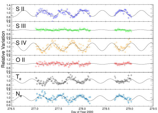
Figure 1: Steffl et al.
Relative ion mixing ratios, electron temperature, and electron column density for a typical 3-day period obtained from the dusk ansa. Values are normalized to the average value over the 3-day period. The best-fit sinusoids for this period are overplotted. Note the strong anti-correlation of S II with S IV and equatorial electron temperature with equatorial electron column density. Figure taken from Steffl et al. (2006).

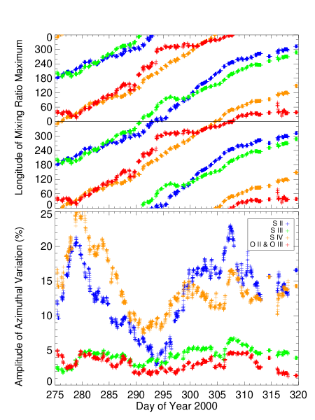
Figure 2: Steffl et al.
Azimuthal variations in the Io plasma torus as observed by Cassini UVIS. The top panel shows the location (in System III coordinates) of the peak in mixing ratio of the primary ion species in the Io torus as a function of time. All four ion species show a roughly linear trend of increasing phase with time. The bottom panel shows the relative amplitude (as a percentage) of the azimuthal variations as a function of time. The relative amplitudes of O II and S III remain around the few percent level, while the comparatively less abundant ion species S II and S IV vary between 4–25%. Adapted from Steffl et al. (2006).

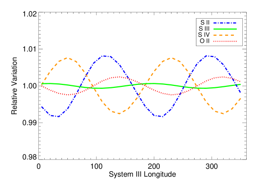
Figure 3: Steffl et al.
Relative variation in torus composition produced by the basic azimuthal model. The small azimuthal variations are caused by the offset between the centrifugal and rotational equators and are therefore double-peaked.

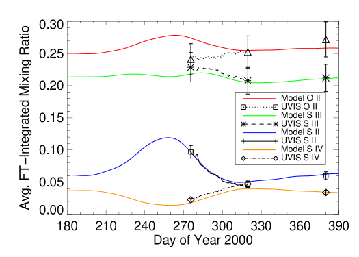
Figure 4: Steffl et al.
Azimuthally-averaged composition of the Io torus as observed by Cassini UVIS and reproduced by the time-variable azimuthal model. Observed mixing ratios derived from UVIS spectra are shown with plot symbols and the thin connecting lines. Uncertainties in the UVIS-derived mixing ratios are approximately 10%, as shown by the error bars. Averaged mixing ratios produced by the time-variable azimuthal model are shown with thick solid lines. Although the model results shown here were produced by the time-variable azimuthal model, virtually identical results can be produced by the subcorotating hot electron model (Section 2.3) and the dual hot electron model (Section 2.4).

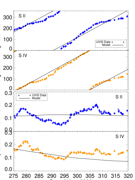
Figure 5: Steffl et al.
Comparison of Cassini UVIS data with output from the subcorotating hot electron model. UVIS observations of both dawn and dusk ansae have been averaged together. The top panel shows the azimuthal location (in System III coordinates) of the peak mixing ratios of S II and S IV. The bottom panel shows the amplitude of S II and S IV azimuthal variations.

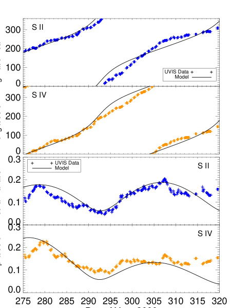
Figure 6: Steffl et al.
Comparison of Cassini UVIS data with output from the dual hot electron model. This model features the superposition of two azimuthal variations in hot electron fraction, one with a rotation period of 10.07 hours and the other with the System III rotation period of 9.925 hours. Unlike the azimuthal variations produced by the subcorotating hot electron model (Fig 5) the phase of the azimuthal variation increases more rapidly when the amplitude is near its minimum value (near DOY 293). The bottom panel shows the amplitude of azimuthal variations of S II and S IV. The interference of the two hot electron variations creates a beat period of 28.8 days.

Figure 7: Steffl et al.
Lomb-Scargle periodograms of the mixing ratio of S II as derived from Cassini UVIS data (left) and the dual hot electron model (right). Model mixing ratios have been sampled at the same time and spatial location as the UVIS observations. Both data and model periodograms show a sharp peak at a frequency of 0.0993 h^-1, corresponding to the 10.07-hour “System IV” period observed by Cassini UVIS and a secondary peak at the System III rotational frequency. Sidebands of the two peaks can be seen near 0.05 h^-1 and 0.20 h^-1. Small spurious peaks due to the sampling interval of the UVIS data are also present.

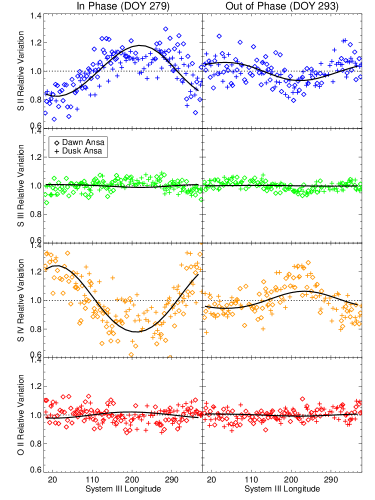
Figure 8: Steffl et al.
Azimuthal variation of ion mixing ratios in the Io plasma torus during two 2-day periods. Plotting symbols represent ion mixing ratios derived from Cassini UVIS data: diamonds from the dawn ansa and pluses from the dusk ansa. The solid lines are output from the dual hot electron variation model.

References

- Bagenal (1994) Bagenal, F., 1994. Empirical model of the Io plasma torus: Voyager measurements. J. Geophys. Res. 99, 11043–11062.
- Barbosa (1985) Barbosa, D. D., Mar. 1985. Thermalization of neutral-beam-injected ions by lower hybrid waves in Jupiter’s magnetosphere. Physical Review Letters 54, 1160–1162.
- Barbosa (1994) Barbosa, D. D., 1994. Neutral cloud theory of the jovian nebula: Anomalous ionization effect of superthermal electrons. Astrophys. J. 430, 376–386.
- Barbosa et al. (1983) Barbosa, D. D., Coroniti, F. V., Eviatar, A., 1983. Coulomb thermal properties and stability of the Io plasma torus. Astrophys. J. 274, 429–442.
- Bell et al. (1983) Bell, K. L., Gilbody, H. B., Hughes, J. G., Kingston, A. E., Smith, F. J., Oct. 1983. Recommended Data on the Electron Impact Ionization of Light Atoms and Ions. Journal of Physical and Chemical Reference Data 12, 891–916.
- Brown (1994a) Brown, M. E., 1994a. Observation of mass loading in the Io plasma torus. Geophys. Res. Lett. 21, 847–850.
- Brown (1994b) Brown, M. E., 1994b. The structure and variability of the Io plasma torus. Ph.D. thesis, University of California, Berkeley.
- Brown (1995) Brown, M. E., 1995. Periodicities in the Io plasma torus. J. Geophys. Res. 100, 21683–21696.
- Brown and Bouchez (1997) Brown, M. E., Bouchez, A. H., 1997. The response of Jupiter’s magnetosphere to an outburst on Io. Science 278, 268–271.
- Brown (1983) Brown, R. A., 1983. Observed departure of the Io plasma torus from rigid corotation with Jupiter. Astrophys. J. 268, L47–L50.
- Burger (2003) Burger, M. H., October 2003. Io’s neutral clouds: From the atmosphere to the plasma torus. Ph.D. thesis, University of Colorado at Boulder).
- Burger and Johnson (2004) Burger, M. H., Johnson, R. E., Oct. 2004. Europa’s neutral cloud: morphology and comparisons to Io. Icarus 171, 557–560.
- Clarke et al. (2004) Clarke, J. T., Grodent, D., Cowley, S. W. H., Bunce, E. J., Zarka, P., Connerney, J. E. P., Satoh, T., 2004. Jupiter’s aurora. Jupiter. The Planet, Satellites and Magnetosphere, pp. 639–670.
- Crary (1997) Crary, F. J., Jan. 1997. On the generation of an electron beam by Io. J. Geophys. Res.102, 37–50.
- Crary et al. (1996) Crary, F. J., Bagenal, F., Ansher, J. A., Gurnett, D. A., Kurth, W. S., 1996. Anisotropy and proton density in the Io plasma torus derived from whistler wave dispersion. J. Geophys. Res. 101, 2699–2706.
- Cummings et al. (1980) Cummings, W. D., Dessler, A. J., Hill, T. W., 1980. Latitudinal oscillations of plasma within the Io torus. J. Geophys. Res. 85, 2108–2114.
- Delamere and Bagenal (2003) Delamere, P. A., Bagenal, F., jul 2003. Modeling variability of plasma conditions in the Io torus. Journal of Geophysical Research (Space Physics) 108 (A7), 5–1.
- Delamere et al. (2005) Delamere, P. A., Bagenal, F., Steffl, A., Dec. 2005. Radial variations in the Io plasma torus during the Cassini era. Journal of Geophysical Research (Space Physics) 110 (A9), 12223–12236.
- Delamere et al. (2004) Delamere, P. A., Steffl, A., Bagenal, F., Oct. 2004. Modeling temporal variability of plasma conditions in the Io torus during the Cassini era. Journal of Geophysical Research (Space Physics) 109, 10216–10224.
- Dere et al. (1997) Dere, K. P., Landi, E., Mason, H. E., Fossi, B. C. M., Young, P. R., 1997. CHIANTI–an atomic dataset for emission lines. Astron. Astrophys. Supp. 125, 149–173.
- Dessler (1985) Dessler, A. J., 1985. Differential rotation of the magnetic fields of gaseous planets. Geophys. Res. Lett. 12, 299–302.
- Esposito et al. (2004) Esposito, L. W., Barth, C. A., Colwell, J. E., Lawrence, G. M., McClintock, W. E., Stewart, A. I. F., Keller, H. U., Korth, A., Lauche, H., Festou, M. C., Lane, A. L., Hansen, C. J., Maki, J. N., West, R. A., Jahn, H., Reulke, R., Warlich, K., Shemansky, D. E., Yung, Y. L., Jan. 2004. The Cassini Ultraviolet Imaging Spectrograph Investigation. Space Science Reviews 115, 299–361.
- Feldman et al. (2001) Feldman, P. D., Ake, T. B., Berman, A. F., Moos, H. W., Sahnow, D. J., Strobel, D. F., Weaver, H. A., Young, P. R., 2001. Detection of chlorine ions in the Far Ultraviolet Spectroscopic Explorer spectrum of the Io plasma torus. Astrophys. J. 554, L123–L126.
- Feldman et al. (2004) Feldman, P. D., Strobel, D. F., Moos, H. W., Weaver, H. A., Jan. 2004. The Far-Ultraviolet Spectrum of the Io Plasma Torus. ApJ601, 583–591.
- Frank and Paterson (2000) Frank, L. A., Paterson, W. R., 2000. Observations of plasmas in the Io torus with the Galileo spacecraft. J. Geophys. Res. 105, 16017–16034.
- Geissler et al. (2004) Geissler, P., McEwen, A., Phillips, C., Keszthelyi, L., Spencer, J., May 2004. Surface changes on Io during the Galileo mission. Icarus 169, 29–64.
- Hill et al. (1974) Hill, T. W., Dessler, A. J., Michel, F. C., 1974. Configuration of the jovian magnetosphere. Geophys. Res. Lett. 1, 3–6.
- Horne and Baliunas (1986) Horne, J. H., Baliunas, S. L., Mar. 1986. A prescription for period analysis of unevenly sampled time series. ApJ302, 757–763.
- Hübner et al. (1992) Hübner, W. F., Keady, J. J., Lyon, S. P., Sep. 1992. Solar photo rates for planetary atmospheres and atmospheric pollutants. Ap&SS195, 1–289.
- Krüger et al. (2003) Krüger, H., Geissler, P., Horányi, M., Graps, A. L., Kempf, S., Srama, R., Moragas-Klostermeyer, G., Moissl, R., Johnson, T. V., Grün, E., Nov. 2003. Jovian dust streams: A monitor of Io’s volcanic plume activity. Geophys. Res. Lett.30, 3–1.
- Küppers and Schneider (2000) Küppers, M., Schneider, N. M., 2000. Discovery of chlorine in the Io torus. Geophys. Res. Lett. 27, 513–516.
- Lennon et al. (1988) Lennon, M. A., Bell, K. L., Gilbody, H. B., Hughes, J. G., Kingston, A. E., Murray, M. J., Smith, F. J., Jul. 1988. Recommended Data on the Electron Impact Ionization of Atoms and Ions: Fluorine to Nickel. Journal of Physical and Chemical Reference Data 17, 1285–1363.
- Lichtenberg et al. (2001) Lichtenberg, G., Thomas, N., Fouchet, T., Dec. 2001. Detection of S(IV) 10.51 m emission from the Io plasma torus. J. Geophys. Res.106 (15), 29899–29910.
- Lomb (1976) Lomb, N. R., Feb. 1976. Least-squares frequency analysis of unequally spaced data. Ap&SS39, 447–462.
- Mazzotta et al. (1998) Mazzotta, P., Mazzitelli, G., Colafrancesco, S., Vittorio, N., Dec. 1998. Ionization balance for optically thin plasmas: Rate coefficients for all atoms and ions of the elements H to NI. A&AS133, 403–409.
- McGrath and Johnson (1989) McGrath, M. A., Johnson, R. E., Mar. 1989. Charge exchange cross sections for the Io plasma torus. J. Geophys. Res.94 (13), 2677–2683.
- Mendillo et al. (2004) Mendillo, M., Wilson, J., Spencer, J., Stansberry, J., Aug. 2004. Io’s volcanic control of Jupiter’s extended neutral clouds. Icarus 170, 430–442.
- Meyer-Vernet et al. (1995) Meyer-Vernet, N., Moncuquet, M., Hoang, S., 1995. Temperature inversion in the Io plasma torus. Icarus 116, 202–213.
- Nahar (1995) Nahar, S. N., Dec. 1995. Electron-Ion Recombination Rate Coefficients for Si I, Si II, S II, S III, C II, and C-like Ions C I, N II, O III, F IV, Ne V, Na VI, Mg VII, Al VIII, Si IX, and S XI. ApJS101, 423–434.
- Nahar (1996) Nahar, S. N., Sep. 1996. Electron-Ion Recombination Rate Coefficients for Si I, Si II, S II, S III, C II, and C-like Ions C I, N II, O III, F IV, Ne V, Na VI, Mg VII, Al VIII, Si IX, and S XI: Erratum. ApJS106, 213–214.
- Nahar (1999) Nahar, S. N., Jan. 1999. Electron-Ion Recombination Rate Coefficients, Photoionization Cross Sections, and Ionization Fractions for Astrophysically Abundant Elements. II. Oxygen Ions. ApJS120, 131–145.
- Osterbrock (1989) Osterbrock, D. E., 1989. Astrophysics of gaseous nebulae and active galactic nuclei. University Science Books, Mill Valley, California.
- Pontius et al. (1998) Pontius, D. H., Wolf, R. A., Hill, T. W., Spiro, R. W., Yang, Y. S., Smyth, W. H., 1998. Velocity shear impoundment of the Io plasma torus. J. Geophys. Res. 103, 19935–19946.
- Porco et al. (2003) Porco, C. C., West, R. A., McEwen, A., Del Genio, A. D., Ingersoll, A. P., Thomas, P., Squyres, S., Dones, L., Murray, C. D., Johnson, T. V., Burns, J. A., Brahic, A., Neukum, G., Veverka, J., Barbara, J. M., Denk, T., Evans, M., Ferrier, J. J., Geissler, P., Helfenstein, P., Roatsch, T., Throop, H., Tiscareno, M., Vasavada, A. R., Mar. 2003. Cassini Imaging of Jupiter’s Atmosphere, Satellites, and Rings. Science 299, 1541–1547.
- Press et al. (1992) Press, W. H., Teukolsky, S. A., Vetterling, W. T., Flannery, B. P., 1992. Numerical recipes in FORTRAN. The art of scientific computing. Cambridge: University Press, 2nd ed.
- Rego et al. (1999) Rego, D., Prangé, R., Ben Jaffel, L., Mar. 1999. Auroral Lyman and bands from the giant planets 3. Lyman spectral profile including charge exchange and radiative transfer effects and color ratios. J. Geophys. Res.104, 5939–5954.
- Richardson and Siscoe (1981) Richardson, J. D., Siscoe, G. L., 1981. Factors governing the ratio of inward to outward diffusing flux of satellite ions. J. Geophys. Res. 86, 8485–8490.
- Roesler et al. (1984) Roesler, F. L., Scherb, F., Oliversen, R. J., Feb. 1984. Periodic intensity variation in (SIII) 9531 A emission from the Jupiter plasma torus. Geophys. Res. Lett.11, 128–130.
- Sandel and Dessler (1988) Sandel, B. R., Dessler, A. J., 1988. Dual periodicity of the jovian magnetosphere. J. Geophys. Res. 93, 5487–5504.
- Scargle (1982) Scargle, J. D., Dec. 1982. Studies in astronomical time series analysis. II - Statistical aspects of spectral analysis of unevenly spaced data. ApJ263, 835–853.
- Schreier et al. (1998) Schreier, R., Eviatar, A., Vasyliunas, V. M., 1998. A two-dimensional model of plasma transport and chemistry in the jovian magnetosphere. J. Geophys. Res. 103, 19901–19914.
- Scudder et al. (1981) Scudder, J. D., Sittler, E. C., Bridge, H. S., Sep. 1981. A survey of the plasma electron environment of Jupiter - A view from Voyager. J. Geophys. Res.86, 8157–8179.
- Shemansky (1988) Shemansky, D. E., 1988. Energy branching in the Io plasma torus - The failure of neutral cloud theory. J. Geophys. Res. 93, 1773–1784.
- Shull and van Steenberg (1982) Shull, J. M., van Steenberg, M., Jan. 1982. The ionization equilibrium of astrophysically abundant elements. ApJS48, 95–107.
- Siscoe and Summers (1981) Siscoe, G. L., Summers, D., 1981. Centrifugally driven diffusion of iogenic plasma. J. Geophys. Res. 86, 8471–8479.
- Sittler and Strobel (1987) Sittler, E. C., Strobel, D. F., 1987. Io plasma torus electrons: Voyager 1. J. Geophys. Res. 92, 5741–5762.
- Smith et al. (1988) Smith, R. A., Bagenal, F., Cheng, A. F., Strobel, D. F., 1988. On the energy crisis in the Io plasma torus. Geophys. Res. Lett. 15, 545–548.
- Smith and Strobel (1985) Smith, R. A., Strobel, D. F., 1985. Energy partitioning in the Io plasma torus. J. Geophys. Res. 90, 9469–9493.
- Smyth and Marconi (2000) Smyth, W. H., Marconi, M. K., 2000. Io’s oxygen source: Determination from ground-based observations and implications for the plasma torus. J. Geophys. Res. 105, 7783–7792.
- Smyth and Marconi (2003) Smyth, W. H., Marconi, M. L., Nov. 2003. Nature of the iogenic plasma source in Jupiter’s magnetosphere I. Circumplanetary distribution. Icarus 166, 85–106.
- Smyth and Marconi (2005) Smyth, W. H., Marconi, M. L., Jul. 2005. Nature of the iogenic plasma source in Jupiter’s magnetosphere. Icarus 176, 138–154.
- Southwood and Kivelson (1989) Southwood, D. J., Kivelson, M. G., Jan. 1989. Magnetospheric interchange motions. J. Geophys. Res.94 (13), 299–308.
- Spencer et al. (2000) Spencer, J. R., Jessup, K. L., McGrath, M. A., Ballester, G. E., Yelle, R., May 2000. Discovery of Gaseous S2 in Io’s Pele Plume. Science 288, 1208–1210.
- Stallard et al. (2001) Stallard, T., Miller, S., Millward, G., Joseph, R. D., Dec. 2001. On the Dynamics of the Jovian Ionosphere and Thermosphere. I. The Measurement of Ion Winds. Icarus 154, 475–491.
- Steffl (2005) Steffl, A. J., May 2005. The Io plasma torus during the Cassini encounter with Jupiter: Temporal, radial and azimuthal variations. Ph.D. thesis, University of Colorado at Boulder.
- Steffl et al. (2004b) Steffl, A. J., Bagenal, F., Stewart, A. I. F., nov 2004b. Cassini UVIS observations of the Io plasma torus. II. Radial variations. Icarus 172, 91–103.
- Steffl et al. (2006) Steffl, A. J., Delamere, P. A., Bagenal, F., Jan. 2006. Cassini UVIS observations of the Io plasma torus. III. Observations of Temporal and Azimuthal Variability. Icarus 180, 124–140.
- Steffl et al. (2004a) Steffl, A. J., Stewart, A. I. F., Bagenal, F., nov 2004a. Cassini UVIS observations of the Io plasma torus. I. Initial results. Icarus 172, 78–90.
- Su et al. (2006) Su, Y.-J., Jones, S. T., Ergun, R. E., Bagenal, F., Parker, S. E., Delamere, P. A., Lysak, R. L., Jun. 2006. Io-Jupiter interaction: Alfvén wave propagation and ionospheric Alfvén resonator. Journal of Geophysical Research (Space Physics) 111, 6211–.
- Swift (2006) Swift, D. W., Dec. 2006. A two-dimensional particle-code simulation of inertial Alfven waves and auroral electron acceleration. AGU Fall Meeting Abstracts, B314.
- Thomas et al. (2004) Thomas, N., Bagenal, F., Hill, T. W., Wilson, J. K., 2004. The Io neutral clouds and plasma torus. In: Jupiter. The planet, satellites and magnetosphere. Edited by Fran Bagenal, Timothy E. Dowling, William B. McKinnon. Cambridge University Press. pp. 561–591.
- Thomas et al. (2001) Thomas, N., Lichtenberg, G., Scotto, M., 2001. High-resolution spectroscopy of the Io plasma torus during the Galileo mission. J. Geophys. Res. 106, 26277–26292.
- Thorne et al. (1997) Thorne, R. M., Armstrong, T. P., Stone, S., Williams, D. J., McEntire, R. W., Bolton, S. J., Gurnett, D. A., Kivelson, M. G., 1997. Galileo evidence for rapid interchange transport in the Io torus. Geophys. Res. Lett. 24, 2131–2134.
- Tokar et al. (1982) Tokar, R. L., Gurnett, D. A., Bagenal, F., 1982. The proton concentration in the vicinity of Io plasma torus. J. Geophys. Res. 87, 10395–10400.
- Voronov (1997) Voronov, G. S., 1997. A Practical Fit Formula for Ionization Rate Coefficients of Atoms and Ions by Electron Impact: Z = 1-28. Atomic Data and Nuclear Data Tables 65, 1–35.
- Wang et al. (1998a) Wang, K., Thorne, R. M., Horne, R. B., Kurth, W. S., Jul. 1998a. Cold torus whistlers: An indirect probe of the inner jovian plasmasphere. J. Geophys. Res.103, 14987–14994.
- Wang et al. (1998b) Wang, K., Thorne, R. M., Horne, R. B., Kurth, W. S., Jul. 1998b. Constraints on jovian plasma properties from a dispersion analysis of unducted whistlers in the warm Io torus. J. Geophys. Res.103, 14979–14986.
- Yang et al. (1991) Yang, Y. S., Dessler, A. J., Sandel, B. R., Mar. 1991. Is System IV independent of System III? J. Geophys. Res.96, 3819–3824.
- Young et al. (2003) Young, P. R., Zanna, G. D., Landi, E., Dere, K. P., Mason, H. E., Landini, M., 2003. CHIANTI - an atomic database for emission lines - Paper VI: Proton rates and other improvements. Astrophys. J. 144, 135–152.
- Zarka et al. (2001) Zarka, P., Queninnec, J., Crary, F. J., 2001. Low-frequency limit of jovian radio emissions and implications on source locations and Io plasma wake. Planet. Spa. Sci. 49, 1137–1149.