Crossover from weak localization to Shubnikov-de Haas oscillations in a high mobility 2D electron gas

Abstract

We study the magnetoresistance, $\delta\rho_{xx}(B)/\rho_{0}$, of a high-mobility 2D electron gas in the domain of magnetic fields, $B$, intermediate between the weak localization and the Shubnikov-de Haas oscillations, where $\delta\rho_{xx}(B)/\rho_{0}$ is governed by the interaction effects. Assuming short-range impurity scattering, we demonstrate that in the second order in the interaction parameter, $\lambda$, a linear $B$-dependence, $\delta\rho_{xx}(B)/\rho_{0}\sim\lambda^{2}\omega_{c}/E_{F}$ with temperature-independent slope emerges in this domain of $B$ (here $\omega_{c}$ and $E_{F}$ are the cyclotron frequency and the Fermi energy, respectively). Unlike previous mechanisms, the linear magnetoresistance is unrelated to the electron executing the full Larmour circle, but rather originates from the impurity scattering via the $B$-dependence of the phase of the impurity-induced Friedel oscillations.

Introduction. There are two prominent regimes of low-temperature magnetotransport in a 2D electron gas: weak localization hikami80 and Shubnikov-de Haas oscillations. Weak localization correction dominates magnetoconductivity at low fields, $\omega_{c}\tau<\omega_{c}^{tr}\tau$, where $\tau$ is the impurity scattering time. Characteristic frequency, $\omega_{c}^{tr}$, is determined from the condition dyakonov94 that the magnetic flux through a triangle with a side of a mean free path, $l=v_{\mbox{\tiny F}}\tau$, is equal to the flux quantum, which yields $\omega_{c}^{tr}\tau=(k_{\mbox{\tiny F}}l)^{-1}$. Here $v_{\mbox{\tiny F}}$ and $k_{\mbox{\tiny F}}$ are the Fermi velocity and Fermi momentum, respectively. On the other hand, the oscillatory in $B$ corrections to the resistivity, $\delta\rho_{xx}(B)=\rho_{xx}(B)-\rho_{0}$, where $\rho_{0}=\sigma_{0}^{-1}=\rho_{xx}(0)=h/e^{2}(k_{\mbox{\tiny F}}l)$, develop at high fields, $\omega_{c}\tau\gtrsim 1$. Thus, the boundaries between the low-field and the high-field regimes are separated by a large parameter, $k_{\mbox{\tiny F}}l$.

The behavior of $\delta\rho_{xx}(B)$ in the crossover regime, $\omega_{c}^{tr}\tau<\omega_{c}\tau<1$ has been studied experimentally for more than two decades, see, e.g., Refs. tsui ; group . It is commonly accepted that this behavior is governed by the interaction effects. More specifically, the $B$-dependence of $\delta\rho_{xx}$ is believed to come exclusively from the inversion of the conductivity tensor houghton82

$$\delta\rho_{xx}^{int}(B,T)\approx\rho_{0}^{2}\left(\omega_{c}^{2}\tau^{2}-1\right)\delta\sigma_{xx}^{int}(T)$$ (1)

where $\delta\sigma_{xx}^{int}(T)$ is the zero-field interaction correction AAL to the conductance. This correction is derived under assumption that, in course of an electron-electron collision, the electron performs many steps $\sim l$ of diffusion; for $\omega_{c}\tau<1$ the orbital effect of $B$ on each step is neglected.

In experiments tsui ; group the electron mobilities were relatively low, so that $k_{\mbox{\tiny F}}l$ was $\lesssim 10$. In the present paper we demonstrate that for very big values of $k_{\mbox{\tiny F}}l\gg 1$, like in Refs. zudov01' ; zudov01 ; mani02 , the higher-order electron-electron interaction processes, at distances $\lesssim l$ are strongly sensitive to $B$ even for $\omega_{c}\tau<1$. Due to these processes, each involving two scattering acts, that were neglected in previous considerations, a lively $B$-dependence of $\delta\sigma_{xx}$ emerges in the crossover domain $\omega_{c}^{tr}<\omega_{c}<\tau^{-1}$. This dependence, in turn, translates into the $B$-dependence of $\delta\rho_{xx}$, which is much stronger than the one coming from the inversion of the conductivity tensor. Namely, we find the interaction contribution to $\sigma_{xx}$ in the form

$$\frac{\delta\sigma_{xx}(B)}{\sigma_{0}}=\frac{4\lambda^{2}}{(k_{\mbox{\tiny F}}l)^{3/2}}\;\text{\Large F}_{1}\left(\frac{\omega_{c}}{\Omega_{l}}\right),~{}~{}~{}\Omega_{l}\tau=(k_{\mbox{\tiny F}}l)^{-1/2},$$ (2)

where $\lambda$ is the dimensionless interaction constant. It is important that the characteristic field, $\Omega_{l}$, lies in the crossover domain, i.e., it is much bigger than $\omega_{c}^{tr}$, but much smaller than $1/\tau$.

The function $\text{\large F}_{1}$ (Fig. 3) has the following asymptotes

$$\text{\Large F}_{1}(x)=\left\{\begin{array}[]{cc}-x^{2}/8,&x\ll 1\qquad\text{(a)}\\ -2x/3,&x\gg 1.\qquad\text{(b)}\end{array}\right.$$ (5)

The new scale of the cyclotron frequencies, $\Omega_{l}$, originates from the new physical process: double backscattering from the impurity-induced Friedel oscillations, see Figs. 1 and 2. By virtue of the fact that this process causes the $B$-dependence of the electron scattering time, the correction Eq. (2) enters also into magnetoresistance, $\delta\rho_{xx}(B)/\rho_{0}$. This magnetoresistance is much stronger than $\omega_{c}^{2}\tau^{2}\delta\sigma_{xx}^{int}(T)$, defined by Eq. (1). Indeed, within a logarithmic factor, $\delta\sigma^{int}/\sigma_{0}\sim\lambda\;(k_{\mbox{\tiny F}}l)^{-1}$. Then it follows from Eqs. (1)-(5) that

$$\frac{\delta\rho_{xx}}{\delta\rho_{xx}^{int}}\sim\left\{\begin{array}[]{cc}\lambda\;(k_{\mbox{\tiny F}}l)^{1/2},&\;\;(k_{\mbox{\tiny F}}l)^{-1}<\omega_{c}\tau<(k_{\mbox{\tiny F}}l)^{-1/2}\\ \lambda\;(\omega_{c}\tau)^{-1},&\;\;(k_{\mbox{\tiny F}}l)^{-1/2}<\omega_{c}\tau<1.\end{array}\right.$$ (8)

We see that in both limits the ratio Eq. (8) is big.

Up to now we considered only low-$T$ behavior of magnetoresistance. With increasing mobility, the condition $T\tau>1$ is met even at low temperatures. Under this condition, the ballistic correction dolgopolov ; Narozhny $\delta\sigma_{xx}^{int}(T)/\sigma_{0}\sim\lambda T/E_{\mbox{\tiny F}}$ is the leading temperature correction to $\delta\sigma_{xx}$. Its origin is the interference between the impurity scattering and the scattering from the Friedel oscillation; linear $T$-dependence results from the fact that, in the ballistic regime, the spatial extent of the Friedel oscillations is limited by the length $r_{\mbox{\tiny T}}=v_{\mbox{\tiny F}}/2\pi T$ rather than by $l$. Since the ballistic correction is merely a $B$-independent renormalization of $\tau$, it does not contribute to $\delta\rho_{xx}$. Instead Mirlin1 , the dependence $\delta\rho_{xx}^{int}(B)$ comes from a small $B$-dependent portion, $\sim\omega_{c}^{2}/T^{2}$, of $\delta\sigma_{xx}^{int}(T)$ yielding $\delta\rho_{xx}^{int}/\rho_{0}\sim\lambda\omega_{c}^{2}/E_{\mbox{\tiny F}}T$.

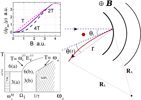
Figure 1: Schematic illustration of electron backscattering from the Friedel oscillation (arcs), created by the short-range impurity (big dot). Magnetic field causes an additional deflection by the angle $\theta_{\mbox{\tiny B}}(r)\approx r/R_{\mbox{\tiny L}}$ due to the trajectory curving and the resulting additional phase $\Psi_{\mbox{\tiny B}}(r)=k_{\mbox{\tiny F}}r^{3}/24R_{\mbox{\tiny L}}^{2}$. Lower inset: domains of different behaviors of $\rho_{xx}$ on the $B$-$T$ plain are shown schematically. Upper inset: evolution of ballistic magnetoresistance with increasing temperature; $\delta\rho_{xx}(B)$ dependencies are plotted from Eqs. (9) and (Crossover from weak localization to Shubnikov-de Haas oscillations in a high mobility 2D electron gas) for three temperatures: $T$, $2T$, and $4T$; Dotted line illustrates a crossover, Eq. (16), from positive to negative magnetoresitance.

Due to the cutoff at distances $\sim r_{\mbox{\tiny T}}$, our result Eq. (2) in the ballistic regime assumes the form

$$\frac{\delta\sigma_{xx}(B)}{\sigma_{0}}\!=\!4\lambda^{2}\left(\frac{\pi T}{E_{\mbox{\tiny F}}}\right)^{3/2}\text{\Large F}_{2}\left(\frac{\omega_{c}}{2\pi^{3/2}\Omega_{\mbox{\tiny T}}}\right),~{}~{}\Omega_{\mbox{\tiny T}}=\frac{T^{3/2}}{E_{\mbox{\tiny F}}^{1/2}},$$ (9)

with characteristic “ballistic” cyclotron frequency, $\Omega_{\mbox{\tiny T}}$, much smaller than the temperature. The asymptotes of the dimensionless function $\text{\large F}_{2}$ are the following

$$\text{\Large F}_{2}(x)=\left\{\begin{array}[]{cc}-0.7x^{2},&x\ll 1\qquad\text{(a)}\\ -2x/3,&x\gg 1.\qquad\text{(b)}\end{array}\right.$$ (12)

Comparison of the corresponding correction to $\rho_{xx}$ with $\delta\rho_{xx}^{int}$ from Ref. Mirlin1 yields

$$\Biggl{(}\frac{\delta\rho_{xx}}{\delta\rho_{xx}^{int}}\Biggr{)}_{T\tau>1}\sim\left\{\begin{array}[]{cc}\lambda\;\bigl{(}E_{\mbox{\tiny F}}/T\bigr{)}^{1/2},&\;\;\omega_{c}<\Omega_{\mbox{\tiny T}}<T\\ \lambda\;\bigl{(}T/\omega_{c}\bigr{)},&\;\;\Omega_{\mbox{\tiny T}}<\omega_{c}<T.\end{array}\right.$$ (15)

For $\lambda\sim 1$ both ratios are big either in parameter $E_{\mbox{\tiny F}}/T$ or in $T/\omega_{c}$, the latter ensures that Shubnikov-de Haas oscillations are smeared out even in the ballistic regime.

The fact that the interaction correction Eq. (9) comes from short distances, $\sim r_{\mbox{\tiny T}}$ suggests that $\omega_{c}\tau$ may be both, smaller or larger than $1$, in the ballistic regime, see Fig. 1, inset. Therefore, one has to use Eq. (1) to transform $\delta\sigma_{xx}(B)$ into magnetoresistance. Then in the “strong-field” domain, $\Omega_{\mbox{\tiny T}}<\omega_{c}<T$, we find from Eq. (9)

$$\delta\rho_{xx}/\rho_{0}=(4/3)\;\lambda^{2}\left(1-\omega_{c}^{2}\tau^{2}\right)\left(\omega_{c}/E_{\mbox{\tiny F}}\right),$$ (16)

i.e., positive magnetoresistance crosses over to negative at $\omega_{c}\tau=3^{-1/2}$. Below we demonstrate the emergence of the new $\omega_{c}$-scales, $\Omega_{l}$ and $\Omega_{\mbox{\tiny T}}$, qualitatively.

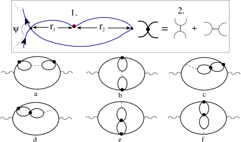
Figure 2: Diagrams for the second-order (in the interaction strength, $\lambda$) correction, $\delta\sigma_{xx}(B)$, to the magnetoconductivity. Diagram $a$ describes combined double scattering from the impurity (big dot) and from the Friedel oscillation; this process is also illustrated in the inset 1, where $\alpha\approx[\theta_{1}+\theta_{\mbox{\tiny B}}(r_{\mbox{\tiny T}})]$ is the net scattering angle, see the text. Two types of four-leg interaction vertices are combined into dots (inset 2).

Qualitative derivation of Eqs. (2), (9). Consider first high temperatures, $T\tau>1$. We will follow the efficient line of reasoning of Refs. Narozhny ; Mirlin1 ; Mirlin2 , which is based on the analysis of the expression for transport scattering time

$$\tau^{-1}=\int d\Theta/2\pi(1-\cos\Theta)|f(\Theta)|^{2},$$ (17)

where $f(\Theta)$ is the full scattering amplitude, $f_{0}(\Theta)+f_{1}(\Theta)$, from the impurity and the impurity-induced potential. Assume a short-range impurity potential, $U_{imp}(r)$. In the first order in interaction strength and for scattering angle $\pi-\Theta=\theta_{1}\ll 1$ (see Fig. 1.) the amplitude $f_{1}$ is given by

$$f_{1}(\theta_{1},T)=-\lambda g\int_{0}^{\infty}\frac{dr}{r}\sin\left(2k_{\mbox{\tiny F}}r\right)A\left(\frac{r}{r_{\mbox{\tiny T}}}\right)$$

$$\times J_{0}\Biggl{(}2k_{\mbox{\tiny F}}r\left[1-\frac{\theta_{1}^{2}}{2}\right]\Biggr{)},$$ (18)

where $J_{0}$ is the Bessel function of zero order, $g=\int d{\bf r}U_{imp}(r)$, and the function $A(x)=x/\sinh x$ is the spatial temperature damping factor (see e.g., Narozhny ). It follows from Eq. (Crossover from weak localization to Shubnikov-de Haas oscillations in a high mobility 2D electron gas) that the characteristic angular interval for the enhanced backscattering is $\theta_{1}\sim(k_{\mbox{\tiny F}}r_{\mbox{\tiny T}})^{-1/2}$. On the other hand, the relative magnitude of enhancement can be estimated from Eq. (Crossover from weak localization to Shubnikov-de Haas oscillations in a high mobility 2D electron gas) as $\left[f_{1}(0,T)-f_{1}(0,0)\right]\sim\lambda f_{0}(k_{\mbox{\tiny F}}r_{\mbox{\tiny T}})^{-1/2}$. Thus, the relative $T$-dependent correction to $\tau^{-1}$ and, correspondingly, to $\sigma_{xx}$, is $\sim\left(\lambda/k_{\mbox{\tiny F}}r_{\mbox{\tiny T}}\right)\sim\lambda T/E_{\mbox{\tiny F}}$, as in Refs. dolgopolov ; Narozhny .

According to Ref. Mirlin1 , incorporating magnetic field into the above picture amounts to adding to the scattering angle, $\theta_{1}$, the angle, $\theta_{\mbox{\tiny B}}(r_{\mbox{\tiny T}})\sim r_{\mbox{\tiny T}}/R_{\mbox{\tiny L}}$, which accounts for the fact that, upon travelling a distance, $r$, in magnetic field, the electron experiences angular deflection by $\theta_{\mbox{\tiny B}}(r)=r/R_{\mbox{\tiny L}}$, see Fig. 1. Here $R_{\mbox{\tiny L}}=v_{\mbox{\tiny F}}/\omega_{c}$ is the Larmour radius. In Ref. Mirlin1 the modification of the amplitude, $f_{1}$, by magnetic field is neglected. Then the effect of $B$ on the scattering rate Eq. (17) reduces to the correction $\sim-\lambda\left[\theta_{\mbox{\tiny B}}(r_{\mbox{\tiny T}})\right]^{2}/\tau$; the factor $\left[\theta_{\mbox{\tiny B}}(r_{\mbox{\tiny T}})\right]^{2}$ comes from integrating $\left[1+\cos(\theta_{1}+\theta_{\mbox{\tiny B}}(r_{\mbox{\tiny T}}))\right]$ over $\theta_{1}$. By noting that $\left[\theta_{\mbox{\tiny B}}(r_{\mbox{\tiny T}})\right]^{2}\sim\omega_{c}^{2}/T^{2}$, we reproduce the result of Ref. Mirlin1 for $\delta\rho_{xx}^{int}(B)$.

The new scale, $\Omega_{\mbox{\tiny T}}$, introduced in Eq.  (9), can be now inferred from the condition, $\theta_{\mbox{\tiny B}}(r_{\mbox{\tiny T}})<\theta_{1}$, that the replacement $\theta_{1}\rightarrow(\theta_{1}+\theta_{\mbox{\tiny B}}(r_{1}))$ in the integrand of Eq. (Crossover from weak localization to Shubnikov-de Haas oscillations in a high mobility 2D electron gas) does not change the amplitude, $f_{1}$. Indeed, equating $\theta_{\mbox{\tiny B}}(r_{\mbox{\tiny T}})$ to $\theta_{1}\sim(k_{\mbox{\tiny F}}r_{\mbox{\tiny T}})^{-1/2}$, we find $\omega_{c}\!=\!T^{3/2}/E_{\mbox{\tiny F}}^{1/2}\!\sim\!\Omega_{\mbox{\tiny T}}$.

It might seem that in the opposite case, $\theta_{\mbox{\tiny B}}(r_{\mbox{\tiny T}})>\theta_{1}$, the size of the scattering region would be determined by the magnetic phase, $\Psi_{\mbox{\tiny B}}(r)$, see Fig. 1 caption, as

$$\!\Psi_{\mbox{\tiny B}}(r_{\mbox{\tiny B}})=\left(k_{\mbox{\tiny F}}r_{\mbox{\tiny B}}^{3}/24R_{\mbox{\tiny L}}^{2}\right)\sim 1,~{}{\text{{ i.e.,}}}~{}r_{\mbox{\tiny B}}\sim(R_{\mbox{\tiny L}}^{2}/k_{\mbox{\tiny F}})^{1/3},$$ (19)

rather than by $r_{\mbox{\tiny T}}$. This, however, is not the case. The reason is that the rigorous treatment we requires incorporating the magnetic phase, $-2\Psi_{\mbox{\tiny B}}(r)$, not only into the argument of the Bessel function in Eq. (Crossover from weak localization to Shubnikov-de Haas oscillations in a high mobility 2D electron gas) but into the argument of sine as well. The latter describes field-induced modification of the Friedel oscillations we . As a result, the $B$-dependent phase factors cancel out.

Our main point is that the cancellation does not occur in the second-order process in the interaction strength. As illustrated in Fig. 2 (inset 1), the backscattering is the result of two virtual scattering processes from the Friedel oscillation. The contribution to the scattering amplitude from this process reads (see also inset 1 in Fig. 2)

$$\tilde{f}_{1}(\theta_{1})=\frac{\lambda^{2}g}{2\pi}\int\frac{d{r}_{1}d{r}_{2}d\varphi_{r_{1}}}{r_{1}r_{2}}A\left(\frac{r_{1}}{r_{\mbox{\tiny T}}}\right)A\left(\frac{r_{2}}{r_{\mbox{\tiny T}}}\right)\qquad$$ (20)

$$\times\sin\bigl{(}2k_{\mbox{\tiny F}}r_{1}\bigr{)}J_{0}\Biggl{(}2k_{\mbox{\tiny F}}|{\bf r}_{1}-{\bf r}_{2}|\left[1-\frac{\theta_{1}^{2}}{2}\right]\Biggr{)}\sin\bigl{(}2k_{\mbox{\tiny F}}r_{2}\bigr{)}.$$

It is seen from Eq. (20) that the characteristic value of the angle, $\pi-\varphi_{r_{1}}$, between ${\bf r}_{1}$ and ${\bf r}_{2}$ is $\sim(k_{\mbox{\tiny F}}r_{1})^{-1/2}$. With magnetic phase $\Psi_{\mbox{\tiny B}}(r)=\left(k_{\mbox{\tiny F}}r^{3}/24R_{\mbox{\tiny L}}^{2}\right)$ included in the arguments of sines and the Bessel function, the slow oscillating term in the integrand of Eq. (20) will acquire the form $-\sin\left[\Phi_{\mbox{\tiny B}}(r_{1},r_{2})-k_{\mbox{\tiny F}}(r_{1}+r_{2})\theta_{1}^{2}+\pi/4\right]$, where

$$\Phi_{\mbox{\tiny B}}(r_{1},r_{2})\!\! = \!\!2\Psi_{\mbox{\tiny B}}(r_{1})+2\Psi_{\mbox{\tiny B}}(r_{2})-2\Psi_{\mbox{\tiny B}}(r_{1}+r_{2})~{}~{}~{}~{}$$

$$= \!\!-k_{\mbox{\tiny F}}r_{1}r_{2}(r_{1}+r_{2})/4R_{\mbox{\tiny L}}^{2}.$$

We are now in position to estimate the $\lambda^{2}$-correction to the scattering rate Eq. (17) in both domains $\omega_{c}<\Omega_{\mbox{\tiny T}}$ and $\omega_{c}>\Omega_{\mbox{\tiny T}}$. For low magnetic field, both $\varphi_{r_{1}}$ and $\theta_{1}$ are $\sim(k_{\mbox{\tiny F}}r_{\mbox{\tiny T}})^{-1/2}$. The integral in Eq. (20) can be estimated as $[\tilde{f}_{1}(\theta_{1},B)-\tilde{f}_{1}(\theta_{1},0)]\sim\lambda^{2}\varphi_{r_{\mbox{\tiny T}}}(k_{\mbox{\tiny F}}r_{\mbox{\tiny T}})^{-1/2}\Phi_{\mbox{\tiny B}}(r_{\mbox{\tiny T}},r_{\mbox{\tiny T}})$. Then the integration over $\theta_{1}$ in Eq. (17) would yield the relative $B$-dependent correction $\sim(k_{\mbox{\tiny F}}r_{\mbox{\tiny T}})^{-3/2}\Phi_{\mbox{\tiny B}}(r_{\mbox{\tiny T}},r_{\mbox{\tiny T}})\sim\lambda^{2}\omega_{c}^{2}/(T^{3/2}E_{\mbox{\tiny F}}^{1/2})$ to the scattering rate. This leads to the estimate $\delta\rho_{xx}(B)/\rho_{0}\sim\lambda^{2}\omega_{c}^{2}/(T^{3/2}E_{\mbox{\tiny F}}^{1/2})$, which coincides with our Eq. (12). For high magnetic fields we have $\varphi_{r_{1}}\sim\theta_{1}\sim(k_{\mbox{\tiny F}}r_{\mbox{\tiny B}})^{-1/2}$; the difference $[\tilde{f}_{1}(\theta_{1},B)-\tilde{f}_{1}(\theta_{1},0)]$ is now $\sim(k_{\mbox{\tiny F}}r_{\mbox{\tiny B}})^{-1}\Phi_{\mbox{\tiny B}}(r_{\mbox{\tiny B}},r_{\mbox{\tiny B}})$, so that the estimate for $\delta\rho_{xx}(B)/\rho_{0}$ assumes the form $\lambda^{2}\omega_{c}/E_{\mbox{\tiny F}}$ again in accord with Eq. (12). Note, that “strong-field”magnetoresistance in the domain $\Omega_{\mbox{\tiny T}}<\omega_{c}<T$ is temperature-independent (see upper inset in Fig. 1).

Consideration for low temperatures leading to Eq. (5) is absolutely similar. On the quantitative level, one has to replace the temperature damping factor $A(r/r_{\mbox{\tiny T}})$ by the probability $\exp(-2r/l)$ that electron does not encounter other impurity in course of scattering from a given impurity and from the Friedel oscillations, created by it.

Outline of the derivation. It is most convenient to calculate the magnetoconductivity, $\delta\sigma_{xx}(B)$, in the coordinate space. In the r-space, Friedel oscillation manifests itself via a polarization operator, $\Pi(r,B)$ , which has the following form we

$$\Pi_{\omega}({\bf r},0)=-\frac{\pi\nu_{0}^{2}\hbar^{4}}{2k_{\mbox{\tiny F}}r}\Biggl{[}i|\omega|+\frac{v_{\mbox{\tiny F}}}{r}\sin\left(2k_{\mbox{\tiny F}}r-\frac{\omega_{c}^{2}E_{\mbox{\tiny F}}\;r^{3}}{6v_{\mbox{\tiny F}}^{3}}\right)$$

$$\times A\Biggl{(}\frac{r}{r_{\mbox{\tiny T}}}\Biggr{)}\Biggr{]}\exp\Biggl{\{}\frac{i|\omega|r}{v_{\mbox{\tiny F}}}-\frac{r}{l}\Biggr{\}},\qquad$$ (22)

where, $\nu_{0}$ is the 2D density of states. The $B$-dependent term in the argument of sine coincides within a numerical factor with magnetic phase, $k_{\mbox{\tiny F}}r\left[\theta_{\mbox{\tiny B}}(r)\right]^{2}$, derived above. Diagram $a$ in Fig. 2 contains two polarization bubbles connected by an impurity line, and positioned in such a way, that they play the role of an effective scatterer. Then the entire diagram $a$ describes the contribution to $\sigma_{xx}$ from the double scattering from the Friedel oscillations. Analytical expression for this diagram in terms of the polarization operator Eq. (Crossover from weak localization to Shubnikov-de Haas oscillations in a high mobility 2D electron gas) is the following

$$\frac{\delta\sigma_{xx}(B)}{\sigma_{0}}=\frac{\lambda^{2}}{\pi\nu_{0}^{4}}\int\!\!d{\bf r}_{1}\!\int\!\!d{\bf r}_{2}\;\left[\frac{1}{\omega}\;\text{Im}\Pi_{\omega}({\bf r}_{1},{\bf r}_{2})\right]_{\omega\rightarrow 0}$$

$$\times\text{Re}\;\Bigl{\{}\Pi_{0}(0,{\bf r}_{1})\Pi_{0}({\bf r}_{2},0)\Bigr{\}},\qquad$$ (23)

where we assumed that the interaction is short-ranged, $V(q)\approx\text{const}(q)=V_{0}$ footnote , so that $\lambda=\nu_{0}V_{0}$. Our “low-temperature” result Eq. (2) emerges upon substitution Eq. (Crossover from weak localization to Shubnikov-de Haas oscillations in a high mobility 2D electron gas) into Eq. (Crossover from weak localization to Shubnikov-de Haas oscillations in a high mobility 2D electron gas), setting $A(r/r_{\mbox{\tiny T}})=1$, extracting a slow term from three rapidly oscillating sines and, finally, performing integration over the azimuthal positions, $\varphi_{{\bf r}_{1}}$, $\varphi_{{\bf r}_{2}}$ of the points ${\bf r}_{1}$, ${\bf r}_{2}$. To arrive to our ballistic result Eq. (9), one should keep $A(r/r_{\mbox{\tiny T}})$ in Eq. (Crossover from weak localization to Shubnikov-de Haas oscillations in a high mobility 2D electron gas) and take the limit $l\rightarrow\infty$. The final form of the dimensionless functions $\text{\large F}_{1}(x)$, $\text{\large F}_{2}(x)$ is the following

$$\!\!\!\!\!\!\!\text{\large F}_{1}(x)\!=\!\frac{1}{\pi^{3/2}}\!\int\limits_{\rho_{1}>\rho_{2}}\!\!\!\frac{d\rho_{1}d\rho_{2}}{(\rho_{1}\rho_{2})^{3/2}}\bigl{\{}\mathcal{H}^{-}(\rho_{1},\rho_{2},x)e^{-2\rho_{1}}$$

$$\qquad\qquad\qquad\qquad+\mathcal{H}^{+}(\rho_{1},\rho_{2},x)e^{-2(\rho_{1}+\rho_{2})}\bigr{\}},$$ (24)

$$\!\!\!\!\!\!\!\text{\large F}_{2}(x)\!=\!\frac{1}{\pi^{3/2}}\!\int\limits_{\rho_{1}>\rho_{2}}\!\!\!\frac{d\rho_{1}d\rho_{2}}{(\rho_{1}\rho_{2})^{3/2}}\bigl{\{}\mathcal{H}^{-}(\rho_{1},\rho_{2},x)A\left(\rho_{1}\right)A\left(\rho_{2}\right)\times$$

$$\!\!\!\!\!\!\!A\left(\rho_{1}\!-\!\rho_{2}\right)+\mathcal{H}^{+}(\rho_{1},\rho_{2},x)A\left(\rho_{1}\right)A\left(\rho_{2}\right)A\left(\rho_{1}\!+\!\rho_{2}\right)\bigr{\}},$$ (25)

where $\mathcal{H}^{\pm}(\rho_{1},\rho_{2},x)=(\rho_{1}\pm\rho_{2})^{-1/2}\{\sin(\pi/4)-\sin[x^{2}\;\rho_{1}\rho_{2}(\rho_{1}\pm\rho_{2})+\pi/4]\}$, and $\pm$ corresponds to ${\bf r}_{1}$, ${\bf r}_{2}$ on the same and opposite sides from ${\bf r}=0$, respectively.

Qualitative derivation pertained to the diagram $a$ in Fig. 2. There are however other virtual, second-order in $\lambda$, processes that give rise to the contributions to $\delta\sigma_{xx}(B,T)$, similar to Eq. (Crossover from weak localization to Shubnikov-de Haas oscillations in a high mobility 2D electron gas). For example, the relevant $\lambda^{2}$ term can come not only from the double backscattering of an electron by Friedel oscillation with magnitude $\lambda$ but also from a direct scattering from an impurity and from “convolution” of the two Friedel oscillations (diagram $c$ in Fig. 2) $\propto\lambda^{2}\int d{\bf r_{1}}\bigl{[}\sin\left(2k_{\mbox{\tiny F}}|{\bf r}-{\bf r}_{1}|\right)/|{\bf r}-{\bf r}_{1}|^{2}\bigr{]}\;\left[\sin\left(2k_{\mbox{\tiny F}}r_{1}\right)/r_{1}^{2}\right]$. Important is that all contributions $\sim\lambda^{2}$ differ only by a numerical factor. Resulting combinatorial factor, $32$, is reflected in Eqs. (2), and (9).

In Fig. 3 we show functions $\text{{\large F}}_{1}(x)$ and $\text{{\large F}}_{2}(x)$ calculated numerically from Eqs. (Crossover from weak localization to Shubnikov-de Haas oscillations in a high mobility 2D electron gas), (Crossover from weak localization to Shubnikov-de Haas oscillations in a high mobility 2D electron gas). Magnetoresistance is related to $\text{{\large F}}_{1,2}$ via additional factor $(\omega_{c}^{2}\tau^{2}-1)$. In accord with qualitative analysis, both functions are quadratic for $x\ll 1$ and linear for $x\gg 1$.

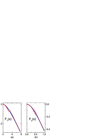
Figure 3: a) Magnetoconductivity, $({\delta\sigma_{xx}}/{\sigma_{0}})[{(k_{\mbox{\tiny F}}l)^{3/2}}/{4\lambda^{2}}]$, at low $T$ is plotted from Eq. (Crossover from weak localization to Shubnikov-de Haas oscillations in a high mobility 2D electron gas) vs. dimensionless magnetic field $x=\omega_{c}/\Omega_{l}$; b) Ballistic magnetoconductivity $({\delta\sigma_{xx}}/{\sigma_{0}})[{E_{\mbox{\tiny F}}^{3/2}}/{4\lambda^{2}T^{3/2}}]$ is plotted from Eq. (Crossover from weak localization to Shubnikov-de Haas oscillations in a high mobility 2D electron gas) vs. dimensionless magnetic field $x=\omega_{c}/(2\pi^{3/2}\Omega_{\mbox{\tiny T}})$. Dashed lines for low fields are the $x\ll 1$ asymptotes in Eqs. (5), (12). Dotted lines illustrate linear behavior of $\delta\sigma_{xx}$ at $x\gtrsim 1$.

Discussion and estimates. Our main result is a novel scale of magnetic fields, $\omega_{c}\tau=(k_{\mbox{\tiny F}}l)^{-1/2}$, and a linear magnetoresistance $\delta\rho_{xx}(B)/\rho_{0}\sim\lambda^{2}\omega_{c}/E_{\mbox{\tiny F}}$ within the interval $(k_{\mbox{\tiny F}}l)^{-1/2}<\omega_{c}\tau<1$. In the samples with moderate mobility tsui ; group $\mu\sim 10^{4}$cm²/V s this interval is narrow, $(k_{\mbox{\tiny F}}l)^{-1/2}\approx 0.3$ for $n=2\cdot 10^{11}$cm^-2 and $\delta\rho_{xx}(B)$-dependencies in tsui ; group are indeed weak and quadratic in the crossover region. By contrast, the data in Refs. zudov01' ; zudov01 ; mani02 for $\mu\gtrsim 2\cdot 10^{6}$cm²/V s exhibit extended intervals of $B$, from $0.02$ Tesla to $0.2$ Tesla, in which $\delta\rho_{xx}$ is strong and linear with either positive or negative slopes. Our theory predicts linear $\delta\rho_{xx}(B)$ only for $\omega_{c}\tau<1$, which was not the case in the above domain of $B$. Throughout the paper we assumed that disorder is short-range. For smooth disorder there exists a specific regime of ballistic magnetotransport, $T\tau>1$, where Shubnikov-de Haas oscillations are suppressed, i.e., $T>\omega_{c}$, but the field is strong, $\omega_{c}\tau>1$. As was demonstrated in Ref. Mirlin2 and confirmed experimentally in Ref. Savchenko , magnetoresistance, $\delta\rho_{xx}/\rho_{0}\sim\lambda(\omega_{c}\tau)^{2}(k_{\mbox{\tiny F}}l)^{-1}(T\tau)^{-1/2}$ in this regime has a distinct $T$-dependence. However, the $B$-dependence still comes from the inversion of the conductivity tensor.

We gratefully acknowledge the discussions with M. A. Zudov and R. R. Du.

References

(1) S. Hikami, A. I. Larkin, and Y. Nagaoka,
Prog. Theor. Phys. 63, 707 (1980).
(2) M. I. Dyakonov, Solid State Commun. 92, 711 (1994);
A. Cassam-Chenai and B. Shapiro, J. Phys. I France 4, 1527
(1994).
(3) M. A. Paalanen, D. C. Tsui, and J. C. M. Hwang,
Phys. Rev. Lett. 51, 2226 (1983); K. K. Choi, D. C. Tsui,
and S. C. Palmateer, Phys. Rev. B 33, 8216 (1986).
(4) W. Poirier, D. Mailly, and M. Sanquer,
Phys. Rev. B 57, 3710 (1998);
P. T. Coleridge, A. S. Sachrajda,
and P. Zawadzki, ibid., 65, 125328 (2002); G. M.
Minkov, et al., ibid., 67, 205306 (2003); E. B.
Olshanetsky, et al., ibid., 68, 085304 (2003);
V. T. Renard, et al., ibid., 72 075313 (2005);
G. M. Minkov, et al., ibid., 74, 045314 (2006).
(5) A. Houghton, J. R. Senna, and S. C. Ying, Phys. Rev. B 25,
2196 (1982).
(6) B. L. Altshuler, A. G. Aronov, and P. A. Lee, Phys. Rev. Lett. 44,
1288 (1980).
(7) M. A. Zudov, et al.,
Phys. Rev. Lett. 86, 3614 (2001).
(8) M. A. Zudov, et al., Phys. Rev. B 64, 201311(R) (2001).
(9) R. G. Mani, et al.,
Nature (London) 420, 646 (2002).
(10) A. Gold and V. T. Dolgopolov, Phys. Rev. B 33, 1076 (1986).
(11) G. Zala, B. N. Narozhny, and I. L. Aleiner, Phys. Rev. B 64, 214204 (2001).
(12) I. V. Gornyi and A. D. Mirlin, Phys. Rev. B 69, 045313 (2004).
(13) I. V. Gornyi and A. D. Mirlin, Phys. Rev. Lett. 90, 076801 (2003).
(14) T. A. Sedrakyan, E. G. Mishchenko, and M. E. Raikh, Phys. Rev. Lett. 99, 036401
(2007).
(15)
Effective interaction constant is expressed through as
, see Fig.
2, inset 2.
(16) L. Li, et al.,
Phys. Rev. Lett. 90, 076802 (2003).