Event Reconstruction and Data Acquisition for the RICE Experiment at the South Pole

Abstract

The RICE experiment seeks to measure ultra-high energy neutrinos ($E_{\nu}>10^{16}$ eV) by detection of the radio wavelength Cherenkov radiation produced by neutrino-ice collisions within Antarctic ice. An array of 16 dipole antennas, buried at depths of 100-400 m, and sensitive over the 100-500 MHz frequency range, has been continuously taking data for the last seven years. We herein describe the design and performance of the RICE experiment’s event trigger and data acquisition system, highlighting elements not covered in previous publications.

I Introduction

The RICE experiment seeks measurement of ultra-high energy (“UHE”; $E_{\nu}>10^{15}$ eV) neutrinos interacting in Antarctic ice, by measurement of the radiowavelength Cherenkov radiation resulting from the collision of a neutrino with an ice molecule. Previous publications described initial limits on the incident neutrino flux(), Kravchenko(2003), calibration procedures(), KravchenkoB(2003), ice properties’ measurements(), Kravchenko(2004), and successor analyses of micro-black hole production(), Hussain(2006), gamma-ray burst production of UHE neutrinos(), Besson(2006), and tightened limits on the diffuse neutrino flux(), Kravchenko(2006).

I.1 Signal Strength

The expected coherent radio pulse from a neutrino-initiated electromagnetic shower in ice was initially derived from the Monte Carlo simulation work of Zas, Halzen and Stanev(), Zas(2006) and more recently explored with other studies, including a variety of simulations building on the ZHS code(), Alvarez-Muniz(2006), GEANT simulations(), Hussain(2004), and an independent time-domain only simulation code(), Butkevich(2006). All simulations model the cascade as it develops in a semi-infinite medium (ice) and calculate the number of atomic electrons swept into the forward-moving cascade as well as the number of shower positrons depleted through annihilation with atomic electrons. From that, one can determine the expected net Cherenkov electric field signal strength at an arbitrary observation point ${\vec{R}}$ by summing the Cherenkov electric field vectors ${\vec{E}}({\vec{R}},\omega)$ for each particle participating in the forward-moving shower. Although simplest in the Fraunoffer approximation, full calculations have also been carried out for receivers in the Fresnel zone(), Buniy(2002). All simulations give the same qualitative conclusion - at large distances, the signal at the antenna is a symmetric pulse, approximately 1-2 ns wide in the time domain. The power spectrum as a function of frequency is approximately linearly rising with frequency, as expected in the long-wavelength limit. In that limit, the excess negative charge in the shower front can be treated as a single (“coherent”) charge emitting Cherenkov radiation with an energy per photon: $E=\hbar\omega$, i.e., $E(\omega)\sim\omega$. Figure 1

Figure 1: Comparison of Institute of Nuclear Research simulation of 100 GeV shower characteristics(), Butkevich(2006) vs. GEANT-4 simulations run at University of Kansas(), Hussain(2004).

shows the status of our current calculations. For perfect signal transmission (no cable signal losses), the signal induced in a 50-Ohm antenna (on the Cherenkov cone) due to a 1 PeV neutrino initiating a shower at R=1 km from an antenna is $\sim$20$\mu$V$\sqrt{B}$, with $B$ the system bandwidth in GHz. This is comparable to the 300 K thermal noise over that bandwidth in the same antenna, prior to amplification. Due to the finite experimental bandwidth, the time domain signal is broadened ($\Delta t\sim 1/B$). Finite bandwidth is introduced by: a) finite response of the antenna, b) cable losses as a function of frequency, which tend to attenuate the high-frequency signal components, c) bandpass filters, which, in the case of RICE, remove $f<$200 MHz to suppress large radiofrequency (RF) noise generated by the AMANDA(/IceCube) photo-tubes. The resulting pulse is therefore stretched in the time domain to $\sim$5 ns.

II Hardware and Signal Path and Experimental Layout

The sensitive detector elements, radio receivers, are submerged at depths of several hundred meters close to the Geographic South Pole. The (Martin A. Pomerantz Observatory) MAPO building houses hardware for several experiments, including the RICE and AMANDA surface electronics, and is centered at (x$\sim$40m, y$\sim-30$m) on the surface. The AMANDA array is located approximately 600 m (AMANDA-A) to 2400 m (AMANDA-B) below the RICE array in the ice; the South Pole Air Shower Experiment (SPASE) is located on the surface at ($x\sim-400$m, $y\sim$0m). The coordinate system conforms to the convention used by the AMANDA experiment; grid North is defined by the Greenwich Meridian and coincides with the +y-direction in the Figure. The geometry of the deployed antennas is presented in Figure 2

Figure 2: RICE antenna deployment geometry.

and also presented in Table 1.

Channel number	x- (m)	y- (m)	z- (m)	time delay (ns)
0	4.8	102.8	-166	1336
1	-56.3	34.2	-213	1416
2	-32.1	77.4	-176	1293
3	-61.4	85.3	-103	1230
4	-56.3	34.2	-152	1166
5	47.7	33.8	-166	1181
6	78.0	13.8	-170	944
7	64.1	-18.3	-171	939
8	43.9	7.3	-171	946
9	64.1	-18.3	-120	809
10	43.9	7.3	-120	672
11	67.5	-39.5	-168	952
12	66.3	74.7	-110	1051
13	-95.1	-38.3	-105	116
14	-46.7	-86.6	-105	1051
15	95.2	12.7	-347	1984
19	-95.1	-38.3	-135	1276

Table 1: Location of RICE radio receivers. We have adopted the coordinate system convention used by the AMANDA collaboration.

A block diagram of the experiment, showing the signal path from in-ice to the surface electronics, is shown in Figure 3. We now discuss in greater detail experimental components not previously discussed in other publications(), Kravchenko(2003, KravchenkoB(2003, Kravchenko(2006).

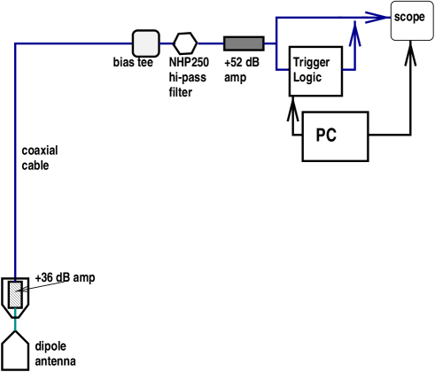
Figure 3: Block diagram, showing primary experimental components.

II.1 Antenna Calibration and Transfer Function

The RICE antennas are “standard” fat dipole antennas, tuned to a center frequency of approximately 450 MHz in air. A sketch of the antenna construction is shown in Figure 4.

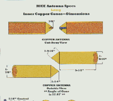
Figure 4: RICE fat dipole antennas.

II.1.1 Antenna Calibration Procedure

We sought to determine a method of antenna calibration, for purposes of predicting signal shape (i.e. voltage amplitude in the time domain) resulting from broadband electromagnetic waves incident on a receiving RICE antenna. This is applicable for radio frequency detectors in situations where the incident field due to events under investigation is predicted by other models, and sensitivity of the detectors to these events must be determined, as is the case for RICE. The complex transmission equation presented here is analogous to the Friis Transmission Formula which is familiar in antenna literature. However, the former, unlike the latter, retains phase information required for predicting signal shape in the time domain. What is needed is the complex transfer function $T$, defined as:

$$V=TE$$ (1)

where $V$ is the voltage output at the antenna terminals, and E is the field incident on the antenna. $T$ depends upon the antenna’s complex effective height(), Farr(1998) $h_{eff}$, its impedance, and the impedance of the load to which the antenna is connected. Of these the complex effective height is difficult to measure directly, but can be calculated using a complex transmission equation, which is analogous to the Friis Transmission Formula familiar in antenna literature. The latter relates input power delivered at the input terminals of a transmitting antenna to the power received at the output terminals of a receiving antenna. Other common parameters characterizing the performance of antenna, (e.g. gain), likewise are defined in terms of power, discarding phase information.

We use a pair of antennas, one transmitting, the other receiving, to extract $h_{eff}$. As the transmission coefficient for a single antenna is readily measured with a network analyzer, then if the complex effective height of one antenna is known, the other may be calculated. Alternatively the complex effective height of two identical antennas may be determined.

II.1.2 Transfer Function

The transfer function relates the output voltage of the antenna to the incident field. Decomposing the field into plane waves in the frequency domain, we can re-cast our definition for $T$ as:

$$V_{\omega}=T_{\omega\theta\phi\rho}E_{\omega\theta\phi\rho}$$ (2)

where $\omega$ is angular frequency, $(\theta,\phi)$ give the polar and azimuthal orientation of the line of propagation of $E$, and $\rho$ gives the polarization of $E$ with respect to the plane made by the axis $\theta=0$ and the line of propagation of $E$

The output signal, the time domain $V_{t}$, is given simply by the Fourier transform of $V_{\omega}$. I.e., the Fourier transform, $T_{t}$ of $T_{\omega}$ is simply a Green’s function for the antenna, characterizing its response to incident waves along a given line of propagation, $(\theta,\phi)$, with a given polarization, $\rho$.

The transfer function is determined by the antenna’s impedance, the load impedance, and the complex effective height of the antenna. The receiving antenna, along with a load (e.g., cable and DAQ electronics) of impedance $Z^{L}$, may be modeled by an equivalent circuit in which the antenna is replaced by a Thevenin generator with an EMF or open circuit voltage, $V^{\mathrm{oc}}$, induced by the incident field, with a series impedance, $Z^{\mathrm{rx}}$. Thus the voltage, $V_{rx}$, at the output of the antenna terminals, and dropped across the load is given by

$$V^{\mathrm{rx}}=\frac{V^{\mathrm{oc}}Z^{\mathrm{L}}}{Z{{}^{\mathrm{L}}}+Z^{\mathrm{rx}}}$$ (3)

where the functional dependence of all variables on the frequency, $\omega$, is implicit.

II.1.3 Complex Effective Height

The complex effective height, in the case of a receiving antenna, relates the incident field to the open circuit voltage of the antenna.

$$V^{\mathrm{oc}}=HE.$$ (4)

Combining the above equations, we can fully characterize the transfer function:

$$T=\frac{HZ^{\mathrm{L}}}{Z^{\mathrm{L}}+Z^{\mathrm{rx}}}.$$ (5)

The complex effective height can also be defined for a transmitting antenna, relating the far field to the current, $I_{tx}$, at the input terminals of the antenna.

$$E_{\mathrm{far~{}field}}=-H^{\mathrm{tx}}I^{\mathrm{tx}}\frac{ie^{{i\omega r}\mathord{\left/{\vphantom{{i\omega r}c}}\right.\kern-1.2pt}c}Z_{0}\omega}{2\pi rc}$$ (6)

where $r$ is the distance, $Z_{0}$ is the characteristic impedance of free space (377$\Omega$), and $c$ is the speed of light. The modulus of $H^{\mathrm{tx}}$ can be interpreted as the length of a uniform linear current segment, centered at the antenna, aligned parallel to the orientation of $E_{\mathrm{far~{}field}}$, with current $I^{\mathrm{tx}}$, which induces the same far field as the antenna in a given direction $(\theta,\phi)$ and polarization $\rho$. The phase angle of $H^{\mathrm{tx}}$ then gives the phase of $E_{\mathrm{far~{}field}}$ due to the antenna relative to the $E_{\mathrm{far~{}field}}$ that would be induced by such a uniform current segment.

There is no immediately obvious relationship between the transmitting and receiving definitions of complex effective height. However, by the Reciprocity Theorem for antennas, the two definitions are in fact equivalent. That is,

$$H_{\omega\theta\phi\rho}^{\mathrm{rx}}=H_{\omega\theta\phi\rho}^{\mathrm{tx}}.$$ (7)

This fact is of particular importance for calibrating a pair of identical antennas of unknown complex effective height. For the remainder of this discussion, we assume reciprocity to be valid. (The accuracy of our full-system gain, ex post facto, validates this assumption, to some degree.)

II.1.4 Complex Transmission Equation

Although it is difficult to measure $E$ in the space near an antenna, the complex transmission coefficient between a transmitting and receiving antenna is readily measured by a network analyzer. What we wish to construct is an equation that relates the complex effective heights, $H^{\alpha}$ and $H^{\beta}$, of a pair of antenna $\alpha$ and $\beta$, to their complex transmission coefficient, $t^{\alpha\beta}$. The complex transmission coefficient is the ratio of the voltage incident on the input terminals of the transmitting antenna, $V^{\mathrm{i}}$, to the voltage output at the terminals of the receiving antenna, $V^{\mathrm{rx}}$. Figure 5 also shows the voltages at the output terminals of the transmitting antenna ($V^{\mathrm{tx}}$) and the input to the receiving antenna ($V^{\mathrm{oc}}$).

Figure 5: Schematic of voltage variables used in equivalent height calculation.

Note that due to reciprocity, it does not matter which antenna is the transmitter and which is the receiver. That is,

$$t^{\alpha\beta}=t^{\beta\alpha}=\frac{V^{\mathrm{rx}}}{V^{\mathrm{i}}}$$ (8)

Before we can construct our complex transmission equation, we must first relate $V^{\mathrm{i}}$ to $I^{\mathrm{tx}}$. First consider the equivalent circuit for a transmitting antenna. In the equivalent circuit the antenna is represented by its impedance, $Z^{\mathrm{tx}}$ in series with a function generator consisting of an ideal AC voltage source, $V^{\mathrm{tx}}$ and a series impedance, $Z^{L}$ (see Fig. 6). The current at the input terminals of the antenna is then given by

$$I^{\mathrm{tx}}=\frac{V^{\mathrm{tx}}}{Z^{\mathrm{L}}+Z^{\mathrm{tx}}}.$$ (9)

At first it may seem that the incident voltage, $V^{\mathrm{i}}$, and the open circuit voltage $V^{\mathrm{tx}}$ of the transmitter’s function generator would be identical. However, the complex transmission coefficient is defined in terms of a voltage wave incident on the interface between the function generator and the transmitting antenna, which gives rise to a reflected and transmitted wave. If we replace the antenna impedance with a zero or infinite impedance (close or open circuit), there will be total reflection, and the magnitude of the reflected wave must equal that of the incident wave, so $V^{\mathrm{tx}}=2V^{\mathrm{i}}$. Thus, in this limit,

$$I^{\mathrm{tx}}=\frac{2V^{\mathrm{i}}}{Z^{\mathrm{L}}+Z^{\mathrm{tx}}}.$$ (10)

Now we can combine equations above to arrive at the complex transmission equation:

$$t^{\alpha\beta}=-H^{\mathrm{tx}}H^{\mathrm{rx}}\frac{2Z^{\mathrm{L}}}{(Z^{\mathrm{L}}+Z^{\mathrm{tx}})(Z^{\mathrm{L}}+Z^{\mathrm{rx}})}\frac{ie^{{i\omega r}\mathord{\left/{\vphantom{{i\omega r}c}}\right.\kern-1.2pt}c}Z_{0}\omega}{2\pi rc},$$ (11)

where $r$ is the distance between the antennas, $Z_{0}$ is the characteristic impedance of free space, and $c$ is the speed of light. Note that we have treated the impedance of the devices at either end as identical, which need not generally be the case, although it typically will be the case if a network analyzer is being used to measure $t^{\alpha\beta}$. In the case where two identical antennas are used, each oriented in the same manner with respect to the other, the complex transmission equation becomes

$$t^{\alpha\alpha}=-(H^{\alpha})^{{}^{2}}\frac{2Z^{\mathrm{L}}}{(Z^{\mathrm{L}}+Z^{\alpha})^{2}}\frac{ie^{{i\omega r}\mathord{\left/{\vphantom{{i\omega r}c}}\right.\kern-1.2pt}c}Z_{0}\omega}{2\pi rc}.$$ (12)

This formalism therefore makes it possible to calibrate a pair of identical antennas. One caveat here is that when solving for $H^{\alpha}$, there is an ambiguity introduced when taking the square root. We resolve this ambiguity by requiring the phase angle of $H_{\omega}^{\alpha}$ to be a continuous function of $\omega$, and also require that the Fourier transform, $H_{t}^{\alpha}$, of $H_{\omega}^{\alpha}$, be causal in the time domain, as it is the Green’s function for the antenna’s open circuit response to the incident wave.

II.1.5 Measurement of Complex Effective Height

Measurement of the complex effective height of an antenna is simply a matter of measuring the antenna’s impedance, then measuring the complex transmission coefficients between pairs of antennas, one of which has known effective height in at least one orientation, or measuring the complex transmission coefficient between a pair of identical antennas which are each oriented in the same manner with respect to the other.

If the environment in which the transmission measurements are taken is not ideal, there may be significant errors introduced by reflections in the environment. Care must be taken to eliminate the error due to reflections by taking multiple transmission measurements and randomizing the effects of reflections. This is done by moving the pair of antennas in tandem, maintaining the same distance and relative orientation, and taking a transmission measurement at each location. In this way the line-of-sight path between the antennas is preserved, while indirect paths due to reflections will be changed with each repositioning of the antenna pair. The range of motion for this procedure should be several times the largest wavelength for which accurate measurements are desired.

II.1.6 The RICE Receivers

The signal path from each antenna to digital oscilloscope consists of the antenna itself, a high pass filter, an amplifier, several hundred meters of coaxial cable, another amplifier, splitter, and finally a digital oscilloscope. We refer to this signal path in its entirety as a ‘receiver’ to distinguish it from the antenna proper, which is simply the first component of the receiver. All components of the receiver, with the exception of the antenna, are impedance matched to 50 ohms to eliminate reflections. We can directly measure a complex transmission coefficient for each component. The product of these with the transfer function of the antenna provides the transfer function for the entire receiver.

Because the receivers are embedded in ice, the index of refraction changes significantly. As a first approximation, we treat the response of the antenna to wavelengths as identical in both media (the validity of this assumption is discussed later in this document). That is,

$$T_{\lambda}^{\mathrm{ice}}=T_{\lambda}^{\mathrm{air}},$$ (13)

where $\lambda={2\pi c}\mathord{\left/{\vphantom{{2\pi c}{n\omega}}}\right.\kern-1.2pt}{n\omega}$, where $c$ is the speed of light and $n$ is the index of refraction of the surrounding medium (air or ice), and we have exchanged the functional dependence of $T$ on $\omega$ for a dependence on $\lambda$.

Figure 6: Equivalent Circuit for a Transmitting or Receiving Antenna.

II.1.7 Measurement of RICE Dipole Transfer Function

To utilize the complex transmission equation, the impedances of the two antennas involved must also be known. Measurement of the impedance of the antennas was also performed using the network analyzer, based on a reflection measurement. The network analyzer measures a reflection coefficient for reflected waves returning via its transmitting port, and the complex impedance of the connected device is directly derivable from the complex reflection coefficient. Note that the impedance measured is, in effect, the lumped impedance of whatever is connected to the analyzer, including effects of its environment. In measuring the antenna impedances, we have assumed that the environment produces negligible reflections returning to the antenna. We have confirmed this by measuring impedance in various locations and found only small variation ($\sim$5 in the VSWR), indicating that reflections from objects in the vicinity of the antenna have little effect on the impedance measurement.

II.1.8 Complex Effective Height Measurement Scheme

The complex effective height of the RICE dipoles was measured using the scheme illustrated in Fig. 7.

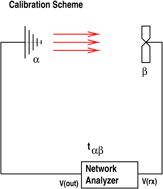
Figure 7: Geometry of effective height measurements for RICE antennas.

A pair of antennas, one transmitting and one receiving, are connected via coaxial cable to a network analyzer, which measures the transmission coefficient (ratio of V^out incident on the input terminals of the transmitting antenna to V^rx output at the terminals of the receiving antenna), as depicted in Fig. 7. The analyzer is calibrated to compensate for the effect of the cables. The measurements were carried out on the roof of the KU Physics Department (Malott Hall) in Lawrence, KS. Given the transmission coefficient and the impedance of both antennsa, the complex effective height is determined using the complex transmission formula.

The complex effective height of two identical Yagi antennas was first measured in this manner. A calibrated Yagi antenna was then used as the standard to measure the complex effective height of two different RICE dipoles. In both cases, the complex transmission equation is used to determine the effective height from the transmission coefficients.

These measurements were taken at a range of 9.38 meters, which corresponds to $r$ in the complex transmission formula. Error in this value has the effect of translating the response of the antenna in time. However, this bias will be identical for all antennas, and as we are ultimately only interested in the relative timing of signal arrival at various antennas, the inclusion of a constant bias in the timing of signals across all antennas will have no effect on our results. We caution that, for wavelengths comparable to the separation distance itself, unprobed Fresnel zone effects may become significant.

II.1.9 Polarization and Incident Angles

The effective height was measured for an incident wave aligned parallel to the axis of the RICE dipole antenna. That is, we have specifically measured $H_{\omega,\frac{\pi}{2},\varphi,0}$. Due to the symmetry of the RICE dipole design, we do not expect significant variation dependent on $\varphi$. For incident angles and polarizations other than this optimal alignment, it has been assumed that $H$ is proportional to $\cos(\alpha)$, where $\alpha$ is the angle between the field vector and the antenna axis ($\alpha$ is a function of $\rho$ and $\theta)$. (Additional measurements suggested that although the $\cos(\alpha)$ relationship is valid for off-vertical polarization angles, it may not be a good approximation for off-horizontal incident angles [i.e., $\theta\neq\pi/2]$. For example, particularly at higher frequencies, the response can actually be greater for $\theta=\pi/4$, than for $\theta=\pi/2$, suggesting a multilobed antenna pattern at the higher frequencies. We estimate that this is a $\sim$10% effect.)

II.2 Results

Fig. 8

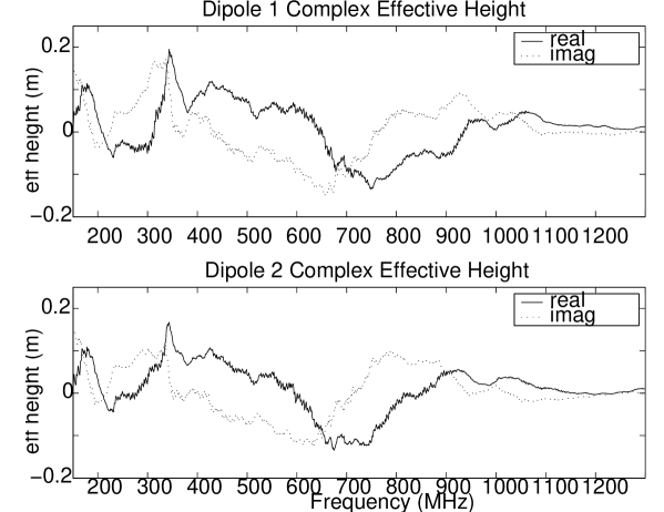
Figure 8: Real and Imaginary parts of RICE complex effective height, measured for two dipole antennas.

shows the complex effective height two different dipoles, indicating the degree of consistency between the two antennas. Fig. 9 displays the complex impedance for the same two dipoles.

Figure 9: Real and Imaginary parts of complex impedance, measured for two RICE dipoles.

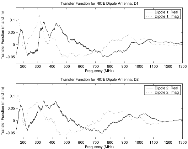
Figure 10: Real and Imaginary parts of transfer function, measured for two RICE dipole antennas coupled to 50$\Omega$ coaxial cable.

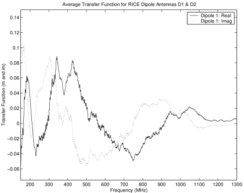
Figure 11: Average transfer function used in Monte Carlo simulations and calculation of neutrino sensitivity.

Fig. 10 shows the transfer functions for these antennas computed from the impedance and complex effective heights, and Fig. 11 shows the average transfer function, which is implemented in the RICE Monte Carlo simulation (‘radiomc’).

II.3 Systematic errors in antenna calibration

It is difficult to obtain an exact value for the amount of error in these measurements for the complex effective heights, impedance, and ultimately the transfer functions of the RICE dipoles. The network analyzer itself performs averaging over several repeated measurements of the transmission or reflection coefficients, which reduce the statistical uncertainty in those measurements to less than $\mathcal{O}$(1%). However, considerable error may be introduced due to reflections in the environment. The amount of error introduced into any single measurement is highly frequency dependent, presumably as a result of whether reflections along different paths tend to reinforce or cancel each other in a given band of frequencies. Of course which frequencies are most affected will also change with the location of the pair of the antennas.

Other random error can be introduced simply by jostling of the antennas as they are repositioned. The distance between antennas can only be maintained to within about 0.1 meter, and their relative orientation to within about 5 degrees. However variation among identical measurements is on the order of two or three percent – much smaller than the error introduced by reflections.

Another source of uncertainty in the calibration of the RICE dipoles is variation among the antennas themselves. We have extensively tested the pair of dipoles mentioned previously. Comparing several antennas, raw reflection coefficient measurements show variations which are typically $\leq$5%.

II.4 Scaling of RICE Dipoles to Ice

Our current assumption is that the transfer function is identical for identical wavelengths. This is equivalent to the statement that the impedance of the environment, having index of refraction n, is given by $\zeta/n$, where $\zeta$ is the impedance of free-space ($\sqrt{\mu_{0}\epsilon_{0}}$=377 $\Omega$). That is,

$$T_{\lambda}^{\mathrm{ice}}=T_{\lambda}^{\mathrm{air}}.$$

Intuitively, if we imagine the antenna as a resonant device analogous to a resonant pipe, the above scaling seems reasonable - if the wavelength through air changes, but the size of the pipe stays the same, then the resoonant frequency will migrate proportionately.

To qualitatively probe environment-dependent antenna response effects, three measurements of the complex reflection coefficient (“S11”) of an antenna in proximity to a large (3 meters across and 1 meter deep) sandbox. The voltage standing-wave ratio (VSWR) was then calculated from the complex reflection coefficient. In the first measurement, a standard RICE dipole was oriented vertically, about 1.5 m above the sandbox. For the second, the dipole was lying horizontally on the surface; for the third, the dipole was dropped about 30 cm into the sand, still oriented horizontally. As indicated in Fig. 12, the peak response migrates from poles at $\sim$350 MHz in air to 250 MHz at the air-sand interface to 215 MHz when buried 30 cm, more or less consistent with the scaling expected by n (expected to be $\sim\sqrt{1.6}$ by $h_{eff}\sim\sqrt{GZ/Z_{0}}$ with the impedance of free space $Z_{0}\to Z_{0}/n$ in a medium of index of refraction $n$).

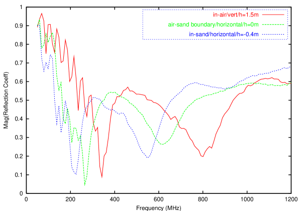
Figure 12: Comparison of antenna VSWR, measured in-sand compared to in-air, as a function of frequency. Note the downward shift in frequency of the peak antenna response.

In our simulations, we determine the expected in-ice response by re-coupling the antenna complex impedance, in medium, to the 50-Ohm coaxial cable.

II.5 Coaxial Cables

Three types of coaxial cables, all having similar attenuation characteristics, connect the in-ice RICE hardware to DAQ electronics in MAPO. With our current detector geometry, we require approximately 200-400 m of cable to reach the DAQ logic in MAPO from the under-ice antennas. A summary of the main cable types and their loss specifications is specified in Table 2.

Type	$v_{\rm propagation}/c$	Power Attenuation(/100’) @ 150 MHz/450 MHz
LMR-500	0.86	1.22 dB/2.17 dB
LMR-600	0.87	0.964 dB/1.72 dB
Cablewave FLC12-50J	0.88	0.845 dB/1.51 dB
Andrews LDF4-50A	0.88	0.73 dB/1.41 dB
Andrews LDF5-50A	0.88	0.46 dB/0.83 dB

Table 2: RICE coaxial cable specifications

II.5.1 Cable Dispersion

In addition to the attenuation characteristics given in Table 2, dispersive effects must also be quantified. Due to increasing signal absorption with frequency, sub-ns duration signals will be “spread” in the time domain as they propagate through our cables. We have directly quantified cable dispersive effects in the frequency domain by measuring the signal propagation time through 800 foot lengths of the LMR-600 and LCF-50J cables, as a function of frequency (Figures 13 and 14). In the RICE passband ($>$200 MHz), the cable is observed to be largely non-dispersive, with phase differences less than 0.25 rad. However, through the passband, the high-pass filter has considerable dispersive effects in the regime 200-300 MHz. Such effects are explicitly incorporated into our simulation.

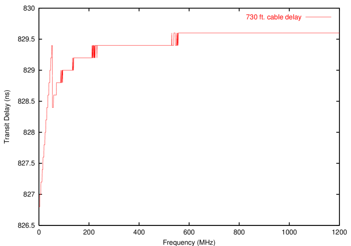
Figure 13: Measured propagation time, as a function of frequency, through $\sim$730 feet of LCF-50J Cablewave cable only.

Figure 14: Measured propagation time, as a function of frequency, through $\sim$840 feet of LMR-600 cable, with high-pass filter connected at one end and terminated into 50$\Omega$. Effect of the high-pass filter is evident for frequencies less than 300 MHz.

II.5.2 Cable Damage during deployment

Following deployment, there is the possibility that the cables are damaged or kinked after freeze-in. Since both our neutrino signal strength, as well as the overall gain calibration depends on the cable signal loss, it is important that any damage to the cable during deployment be minimized. Figure 15 shows the standing-wave-ratio (SWR) obtained for 5 transmitters, frozen into the ice. We note the presence of large returns in 97Tx4, indicating the possibility of damage during freeze-in.

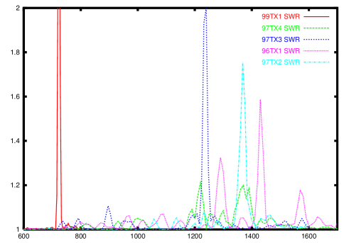
Figure 15: Standing Wave Ratio, all transmitters. Horizontal axis shows time delay (ns) relative to output signal from network analyzer.

II.5.3 Cable cross-talk

Although the RICE coaxial cable should be well-shielded, cross-talk effects may lead to spurious hits recorded in our data. We have, therefore, searched for cross-talk between antennas in the same hole, knowing the spatial difference between any pair of antennas, as well as the signal propagation velocity through the cable. For example, channels 7 and 9 are in the same hole and are separated by approximately 50 m (similarly for channels 8 and 10). Consider two possibilities: a) the deep receiver is hit first, sending a signal up through the cable, which cross-talks to the shallower receiver, within a time scale of 1-2 ns or so. In this model, the time difference between the two signals (original plus induced through cross-talk) received at the surface is very small (the same 1-2 ns, assuming $v_{cable,1}$ =$v_{cable,2}$ and the cable lengths are the same), b) the shallow receiver is hit, a cross-talk signal propagates both up and down the cable attached to the deep receiver. At the surface, we would measure an induced signal in the deep receiver delayed, relative to the former case, by the total extra cable transit time for the deep antenna. Note that $\sim$0 ns observed time difference would also correspond to signals induced in the surface electronics.

II.5.4 Cross-talk due to AMANDA (and RICE) cables

We considered two possible cases - a) cross-talk in holes with AMANDA cables, as well as b) cross-talk in the “dry” holes drilled specifically for RICE. An illustration of the cross-talk geometry is shown in Fig. 16.

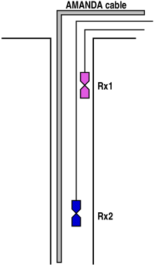
Figure 16: Geometry of possible cross-talk effects.

Channel 1 is 50 m deeper than channel 4 in an AMANDA hole, corresponding to an additional cable time delay of $\sim$190 ns if cross-talk pickup is in the RICE cable itself, and $\sim$280 ns if cross-talk pickup is in the AMANDA cabls. Given the full cable-length time delays (1416 ns, and 1166 ns, respectively), and knowing the cable lengths $l^{\prime}$ and $l$, we would expect the channel 1 signal to arrive at the DAQ either 440 ns, or 530 ns after channel 4 signals if all the channel 1 signals were due to cross-talk effects. For channel 7 and channel 9, we expect channel 7 to arrive 380 ns after channel 9 for complete cross-talk pickup in channel 9. Such bands are not observed in data (Fig. 17).

Figure 17: Hit time registered in channel 1 (x-) vs. hit time registered by hit in channel 4 (y-), for general events. Note that when either channel is the 4th hit of the 4-hit coincidence, its time is set to $\sim 1.5\mu$sec, corresponding to the vertical and horizontal off-diagonal bands.

II.6 Double pulses

Visual scanning of our event sample shows a large fraction of events which contain double pulses. (It is, in fact, the presence of such double pulses which gave rise to some concern that triggered-sampling digitizers may miss pre-trigger or post-trigger double pulses which would otherwise disqualify a hit as ’valid’.) Algorithms which target, and reject such double-pulse events, would also be potentially very worthwhile in our efforts to minimize backgrounds. We have searched for double pulses in two ways: first, by looking at the time-over-threshold distribution, scatter plotted against the time difference between the time-of-first-$6\sigma$-excursion minus the time-of-last-$6\sigma$-excursion (Figure 18), to determine if our backgrounds are characterized by a simple series of high-amplitude signals, having fixed temporal extent. In this model, the pieces of the waveform before and after this background are quiescent. Although Figure 18 does, indeed, show a clear correlation between these two quantities, the fact that the diagonal band in each channel is relatively thick, and not thin, indicates that the temporal extent of the receiver hit has large scatter.

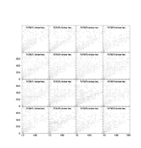
Figure 18: Time over threshold in each channel (horizontal) vs. time difference between last and first $6\sigma$ excursion, in a waveform. “Double pulses”, in which a waveform is repeated multiple times with a fixed time delay between the first and next pulse, should appear as single bin peaks in these plots.

We expect real double pulses due to signals which traverse a “direct” path from source to measurement point, followed by the signal reflected off of the air-surface interface and back down to the antenna. By contrast, noise generated on the surface can travel down the cable, and “reflect” off an antenna back up to the DAQ. Figure 19 shows the expected time delay between the direct and the surface-reflected signals (in nanoseconds) for the case where both transmitter and receiver are at a depth of –150 m, for a given radial separation between transmitter and receiver. Note that the current double pulse cut in the reconstruction code is set to 800 ns, which should cut out very few events resulting from true physical reflections at the air-ice interface.

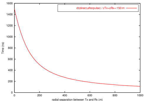
Figure 19: Expected time difference between direct and after pulse (simulation), given indicated transmitter/receiver geometry.

The magnitude of the afterpulse is determined by the additional pathlength (to first order, the signal power $\propto 1/r^{2}$) and the reflection coefficient of the signal at the surface (determined by the appropriate Fresnel coefficients). For the same geometry as assumed in the previous figure, and ignoring any defocusing of the signal as it reflects off the uneven top surface (this is certainly not the correct case), Figure 20 gives the signal strength of the reflected pulse compared to the initial signal strength, based on an analytic calculation just using the Fresnel Reflection Coefficient expected at the surface interface (red, assuming straight line trajectories through the firn), then including $1/r^{2}$ spreading of field lines (green), and compared with one calculation of the current Monte Carlo simulation (point), which includes the differential bending of the ray as it traverses the firn. Note also that these plots assume a spherical source geometry – in the rare instance of a neutrino induced signal, for which a RICE receiver is hit at the Cherenkov angle, the afterpulse would be diminished by the cone angular width factor $\sim exp(-(\theta-\theta_{c})^{2}/(2*(d\theta)^{2})$, with $d\theta\sim$0.04 radians at 500 MHz.

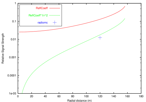
Figure 20: Amplitude of “Reflected” second pulse, based on calculated Fresnel reflection coefficient, compared with ray-tracing code currently used in RICE signal Monte Carlo simulation.

II.6.1 Time Structure of After Pulses

Observations indicate that the after-pulse in a double pulse event occurs typically anywhere from 500 ns – 2000 ns after the initial pulse in an event, and $\sim$10%–50% in amplitude of the initial pulse (for events that saturate, the amplitude could, in principle, be measured simply from the time-over-threshold of the signal, modulo amplifier saturation effects). It was also noticed that after-pulses occur, to some extent, in transmitter data, as well. In several cases, we observe that the time delay between the hit-time of the primary pulse in an event and the after-pulse is of order twice the cable delay between the surface and the transmitter that was broadcasting the signal, consistent with a picture where the source emits a signal which is partially transmitted and partially reflected back to the generator, then subsequently re-reflected down to the transmitter. In fact, laboratory tests performed at KU indicate that the situation is more complicated than that – not only do we observe clearly the (generator$\to$Tx$\to$generator$\to$Tx) reflection, but the (Rx$\to$scope$\to$Rx$\to$scope) reflection is also evident, albeit at a lower amplitude than the former reflection

We have looked in the 2000 data for evidence of double pulses, using the variable t800nXX, where “t800n” indicates that we are examining the first large-amplitude excursion at least 800 ns following the first hit in a waveform, and “XX” designates a channel number. Figure 21 shows the distribution in the time difference between t800nXX and the time of the maximum voltage in a given waveform, for general event triggers. One observes the expected time difference that would correspond to a reflection off the surface electronics itself and back down to the in-ice receiver (i.e. a time difference which is twice the listed time delay for that channel) clearly in channels 6, 7, 8 , 10 and 12. Further investigation shows that the appearance of double pulses is strongly correlated for channels 6, 7, and 8 (i.e., when one channel shows a receiver reflection at the exptected time delay, the other two channels do, as well). In addition, such events show a strong correlation with the vertex location (x,y,z) = (100,–140,0), for both vertexing algorithms, as shown in Figure 22. Although this location does not obviously correspond to a feature on the surface, it is important to remember that ray tracing distortions complicate surface source locations.

Figure 21: Distribution of time difference between time of largest amplitude hit in a given channel relative to time of second largest amplitude hit, requiring that the largest hit be at least 800 ns separated in time from the 2nd hit (general events). Each panel represents an oscilloscope waveform channel, beginning with channel 0 (top) to channel 15 (bottom). Horizontal axis is time in ns.

Figure 22: Vertex distributions, for events which show clear $Rx$ reflections.

As an example of what the time domain waveforms look like for such double pulse events, Figure 23 shows the waveforms observed for event 8, day 196, of the year 2000 data (channels correspond to the ‘index’ indicated in these plots).

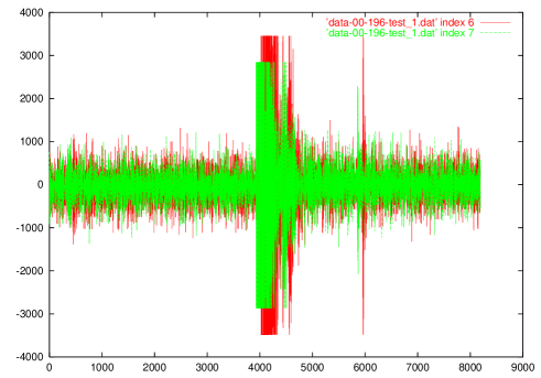
Figure 23: Typical waveforms for events which show “$Rx$”-type reflections, for two channels. (Horizontal axis is time in nanoseconds; vertical scale is arbitrary.) Note that the time difference between first- and second-pulses are comparable for these two channels (channel 6 and 7).

II.6.2 Discriminator Performance

After the cables, the next element in the signal path is the LeCroy 3412 discriminator. Since the neutrino signal has an intrinsic bandwidth of $\sim$1 GHz, the discriminator must be highly efficient for ns-duration RF pulses. A series of studies were conducted to quantify the efficiency of the LeCroy 3412. A fast signal generator (HP8133A), capable of generating 500 ps width signals was used to pulse a 3412 module in the lab; the signal was split and monitored with an HP54542 digital oscilloscope. The nominal threshold of the 3412 is varied by turning a set screw on the front panel of the 3412 module; a voltage probe allows to read back the corresponding threshold value. As shown in Figure 24, the 3412 efficiency turn-on is not sharp; rather, we measure the 3412 set voltages corresponding to initial response, up to 100% efficiency. Down to a signal width (FWHM) of 500 ps, the discriminator performs as expected (to within 10%), and also out-performs the internal trigger of the HP54542.

We have also determined, in the laboratory, that the 3412 discriminator is capable of triggering on a wide range of amplitudes and signal strengths. A test was run for which the 3412 threshold was set to 0.9$\times V_{generator}$, where $V_{generator}$ is the output signal voltage as recorded by an HP8133 signal generator. Figure 24 shows the voltage levels recorded for both the generator, and also as read off one of the RICE HP54542 digital oscilloscopes, for which the trigger efficiency exceeded 90%. We observe good efficiency for signals down to 0.5 ns.

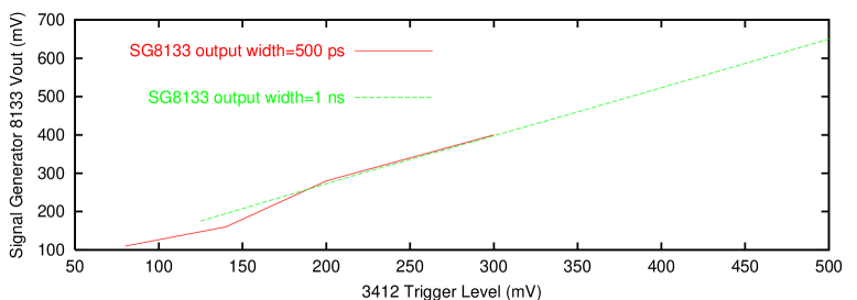
Figure 24: LeCroy 3412E Discriminator efficiency study. The lines correspond to the 3412 Trigger level required for 100% efficiency. Units are millivolts.

II.7 Amplifiers

RICE voltage signals are typically boosted by a factor of $10^{4}$ before waveforms are recorded. Such a large gain requires daily monitoring. We now describe amplifier gain measurements and calibration.

II.7.1 Gain Drift

As described previously(), KravchenkoB(2003, Kravchenko(2006), the amplifier gain is calculated on-line, simply by measuring the rms of the voltage distributions recorded in ‘unbiased’ events, and, after correcting for the known cable losses in each channel, relating the noise power in a bandwidth B to the voltage $V$ by $V^{2}/Z=kTB$, with $Z$ the characteristic impedance of the system. Figure 25 shows the monitored amplifier gains, over a 20-hour period. Figure 26 shows the monitored gains, over a longer time baseline. We estimate the statistical error from each measurement to be of order 1 dB. Some ‘spikes’ are visible, which contribute to our overall systematic error.

Figure 25: Calculated gains, based on normalizing to thermal noise, for “unbiased” triggers, taken from April 15, 2001 data for five (random) channels.

Figure 26: Voltage rms in three RICE channels, monitored over a full-year period; approximately one entry per day.

II.7.2 Amplifier Saturation

At large enough signal input amplitudes, most amplifiers will saturate (roughly, when the output voltage is of order 0.1$\times V_{bias}^{plateau}$, with $V_{bias}^{plateau}$ the bias voltage required for the amplifier to reach it’s maximum gain). By sweeping at either very high power, or fast sweep time, we can probe possible amplifier saturation effects. This is illustrated in Figure 27. We expect linearity, however, for the short-duration excitations induced by neutrino events.

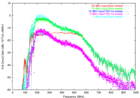
Figure 27: Calculated full-circuit gain (signal generator$\to$transmitter antenna$\to$receiver antenna$\to$surface data acquisition), as a function of network analyzer sweep time. We observe saturation effects at fast sweep times coupled with large input power.

III Online Software

Data are collected online using a custom-written LabView code (running in the Windows environment) which interfaces to the CAMAC hardware and also sets the parameters for the digital oscilloscopes. Runs are initiated daily by the Raytheon Polar Services winter-over (for which we are eternally grateful); data are also archived to CD on a daily basis, as well.

III.1 Trigger scheme

There are three possible conditions that can produce a RICE trigger:

1. The main RICE trigger is a “self-trigger”, which is formed if $\geq$N underground antenna receivers fire over threshold within the 1.25 microsecond gate. At present we use a 4-fold coincidence criterion. These are our primary physics events (“general” trigger events).

2. Random noise triggers, or so called Unbiased events, are triggers forced by the DAQ periodically to sample the noise environment.

3. An AMANDA-B or SPASE coincidence trigger (aka “external” trigger) fires if at least one underground antenna is hit within $\pm$1.25us from the trigger signal received from the “big” AMANDA-B or SPASE. The “big” AMANDA-B trigger signal corresponds to a 30-fold AMANDA multiplicity trigger.

A functional diagram of the DAQ and trigger is presented in Fig. 28.

Figure 28: Functional diagram of the DAQ electronics.

The figure is divided into logical sections by a dotted line. First, consider the Main Rice Trigger. Analog data from antennas arrive at the CAMAC discriminators 3412E and (B). If any channel exceeds the discriminator threshold, a NIM pulse appears at the output of this channel. The “Current Sum Output” for all hit channels of the 3412E is converted into a 1.25$\mu$s long NIM pulse by means of two discriminators 821 A(1) and 821 A(4). Transformed into an ECL signal, this then opens the gate of the MALU 4532 module. While the gate is open, the MALU counts rising edges arriving at its inputs 0-15 from the 3412E (only one hit per channel is counted). If the number of pulses seen by the MALU is greater than or equal to some preset value N (by default, 4), a general trigger pulse is produced by this module.

The Noise Events Trigger produces Unbiased events. The chain for this trigger starts at the Gate 2323A (2). At appropriate moments, this Gate is triggered by the DAQ executable from the main PC through the GPIB interface. Two copies of this signal created using the 821 A(2) module are connected to the “Test” inputs of both discriminators 3412E and B. A pulse appearing at the “Test” input produces hits in all channels of the discriminators’ outputs. These hits then propagate through the remainder of the DAQ as with the Main Rice Trigger. Afterwards, the events develop as described above for the Main Rice Trigger.

The remaining trigger line is the External Trigger, that is, either the AMANDA-B or SPASE coincidence triggers. First, we ensure that the AMANDA and SPASE triggers are standard NIM signals using the discriminators 821 B(1) and 821 B(2). Next, we form a logical OR of AMANDA and SPASE by means of the Logic FIFO (1) module. Then, we want to impose the logical condition $A.and.B=C$ where A is detection of AMANDA or SPASE and B is at least one underground RICE; while C is the result. Since our LFIFO has only OR logic in it, we therefore use the fact that $A.and.B=C$ is logically equivalent to $\bar{A}.or.\bar{B}=\bar{C}$, which is then employed in the FIFO (2) logic. I.e., we take the .OR. of the inverted AMANDA.or.SPASE logic signal and the inverted “at least 1 underground hit” logic signal. We then take an inverted output, corresponding to our desired “C”, External Trigger.

These three chains form the input for the Combined Trigger. The Main RICE trigger is ORed with the External Trigger in the Logic FIFO (3). A Veto can be invoked with the following logic: $A.and.\bar{B}=C$, where A is a valid trigger, B is the veto pulse and C is the final trigger. In the absence of an .AND. module, we use the fact that $A.and.\bar{B}=C$ is equivalent to $\bar{A}.or.B=\bar{C}$. Thus, we combine the inverted result of LFIFO(3) with the plain output of the veto branch in Logic FIFO(4) and take the inverted output of this combination. This output is finally run through 821 C(1) to obtain a constant duration logic pulse. The result is the “raw” RICE trigger. One copy of this is used to monitor the raw trigger rates, connected to an external scalar, e.g. The other copy triggers the gate unit 2323A (1); the output of it is the final RICE trigger. The last unit is needed as it latches the system and preserves the event until it is read out.

The discriminator 821 C(2) produces 5 copies of the final trigger that latch the scopes and freeze the event time in the GPS module. The TDC also receives its “Start” from the final RICE trigger, while data inputs come from the discriminators 3412E and 3412 delayed by 1.5 $\mu$s in the Delay modules A and B.

Once triggered, the system ignores any other possible valid triggers and retains data in the TDC and the scopes until cleared and enabled again.

III.1.1 Software Online Trigger Veto

The second (software) level vetoes time-of-hit patterns for ‘general’ triggers (as registered by on-line DAQ TDC’s) which are characteristic of surface-generated noise. These were determined by simulating sources located at known South Pole science stations in the vicinity of the RICE experiment, including MAPO, the ASTRO, and the SPASE experiments. The resulting hit times were stored in a “library”, which was then compared with an ensemble of expected antenna hit times from simulated neutrino events. This online filter works reasonably well - typical efficiencies of this filter range from 96%–99% (based simply on the ratio of general triggers to rejected veto triggers, assuming that all the general triggers are, in fact, surface in origin). The efficiency, as a function of Julian day, for 2003, is shown in Figure 29.

Figure 29: Calculated surface-source veto efficiency (software), as a function of Julian date (2002).(This is NOT the efficiency for passing neutrino events.)

III.2 Deadtime Determination

III.2.1 Online Live Time monitoring

The Live Time of the DAQ is calculated on-line during data taking. Each event cycle can be roughly broken into two pieces: waiting for event and event processing, as shown in Fig. 30. When the new event arrives, the DAQ does not respond instantly, but with a certain delay. In the process of waiting, the executable stays within a “while” loop, checking for a trigger every cycle as well as performing some other actions. One waiting cycle takes approx. 4-5ms, about 1.2ms of which is actual checking for the trigger occurrence. The definition of the dead/live time is illustrated in Fig. 30. Out of the full time that one event takes, the first “waiting for event” cycle and full “handling event” part is counted as dead time, while the extra (above 1) “waiting for event” cycles are counted as live time. The live fraction is then defined as Live Time divided by the total event time for this event. The total live fraction for the run can now be calculated as the total live time for all events detected divided by the total run time. In addition, the experiment is essentially ‘shut down’ when the South Pole Station uplink (at 303 MHz) to the LES-9 satellite is active (approximately 5 hours out of every day prior to 2005, when LES was disabled by NASA).

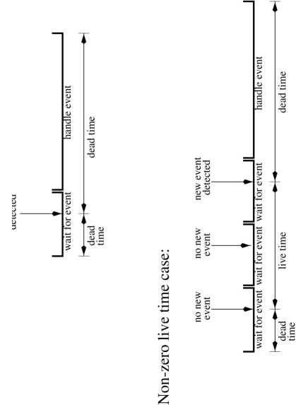
Figure 30: Live/dead time definition

A fair amount of effort was invested in attempting to assess the dead time intrinsic in forming the event trigger, and also associated with making the software veto decision described above, as well as the maximum rates that the DAQ is capable of. There are two areas that have been investigated: the maximum rate at which DAQ can process events and decide whether to accept or reject them, and dead time incurred when a good event is being saved.

III.2.2 Maximum trigger rate

First, we measure the maximum DAQ veto rate and veto dead time. A four-fold copy of signals coming out of a signal generator is sent into the 3412E. The time spacing between the signals is set (using appropriate delays from the PS 794 unit) so that the event should constitute a four-fold coincidence, but the timing pattern should be consistent with a ‘veto’ event. The frequency of the Signal Generator output is then varied, and the trigger rate through the DAQ recorded. If the dead time were zero, then the trigger rate through the DAQ would exactly track the input signal generator rate. The results of this test, for data taken in 2000, are given in Table 3. Subsequent improvements to the DAQ and the CAMAC interface gave approximately four-fold reductions in dead time.

Generator	Fast mode		Slow mode
frequency, Hz	Event Rate, Hz	Live fraction	Event Rate, Hz	Live fraction
10	10.1	0.918	9.9	0.800
20	20.3	0.838	19.7	0.580
30	30.2	0.758	30.2	0.294
40	39.8	0.679	39.9	0.157
50	50.4	0.599	40.1	0.165
60	60.5	0.517	-	-
70	69.1	0.440	34.6	0.228
80	79.4	0.357	-	-
90	89.3	0.279	-	-
100	99.4	0.194	44.2	0.092
105	105.3	0.155	-	-
110	109.9	0.117	-	-
115	114.2	0.078	-	-
120	113.7	0.084	-	-
125	112.0	0.093	-	-
130	105.1	0.148	-	-
135	93.2	0.256	-	-
140	78.0	0.368	-	-
150	80.8	0.346	43.2	0.044
160	79.3	0.356	-	-
170	84.3	0.316	-	-
200	99.9	0.194	-	-
300	100.9	0.188	-	-
400	100.8	0.188	-	-
500	118.3	0.037	-	-
1000	123.4	0.000	-	-
5000	124.9	0.000	48.3	0.000

Table 3: Veto rate as a function of the input frequency of the simulated signal. Slow mode is different from fast mode by the presence of the LabView Event Display window. Unmeasured quantities are indicated by a dash.

From the table, we draw the following conclusions:

• Saturation of the rate happens at about 125 Hz indicating a dead time of 0.008 seconds.

• The event rate is independent of how many scopes/channels are in the system, as expected (the numbers in the table correspond to runs with 16 channels used; the runs with a single channels active give the same result).

• The event rate does not rise monotonically but goes up and down before reaching saturation. This is likely to be caused by the interference between the cycles with different time constants: the frequency of the generator and DAQ polling rate. Naturally, this does not affect the dead time of the system which should be calculated at the rate saturation point.

III.2.3 Calculation of correlation between trigger rate and deadtime (general events)

First, we examine the time between successive triggers (“DTTRIG”, Figure 31). Three peaks are evident - at 10 seconds (the time required to read out general events), 20 seconds (the time required to read out an unbiased event), and t=600 seconds (the time between successive unbiased events, if there are no other intervening triggers). Of the 14136 events in this plot, 10546 of them correspond to DTTRIG$>$20 seconds. Alternately, during this data-taking period $>$70% of our triggers are not occurring in “general-trigger-saturation” mode. Given that these data were taken during IceCube drilling and the ambient noise levels are large, this is not surprising.

Figure 31: Time between successive triggers, all event types, January, 2005 data.

Figure 31 suggests considering whether surface-originating events can also be obviously characterized by their time-since-last-trigger. Events which are saturating the DAQ, such that triggers are being registered as fast as the DAQ can record them, are likely to be of a single origin. For cases of small time-since-last-trigger, we expect the vertices to cluster at the surface, since such times are clearly dominated by background. Figure 32 shows the reconstructed vertices according to time-since-last-trigger. The small time-since-last-trigger events, corresponding to small livetime, cluster around the known location of the MAPO building.

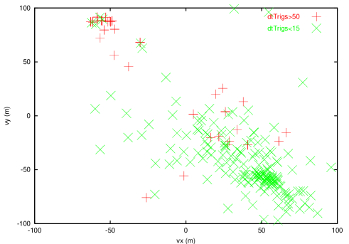
Figure 32: Vertices, 2002 data, divided into subsamples of large time-since-last-trigger, and small time-since-last-trigger. The MAPO building is centered at approximately (x=–50,y=–50) in the Figure.

III.3 HSV board

As discussed elsewhere, an additional Hardware Surface Veto CAMAC board was integrated into the RICE Data Acquisition system beginning in January, 2005(), Kravchenko(2006). For hits separated by at least 20 ns, this board has been measured to provide a veto of potential surface-generated noise at a rate greater than 200 KHz. This board also allows us the capability of measuring singles rates in the RICE antennas (Fig. 33 and also Fig. 34, which shows the possible correlation of the singles rate with large rms values for each channel). We estimate that the HSV board enhances our neutrino sensitivity by $\sim$30-40%.

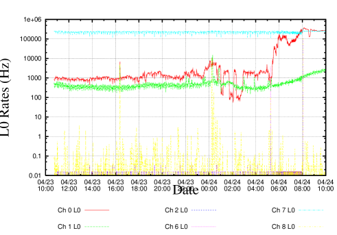
Figure 33: Raw (“Level 0”) HSV singles rates.

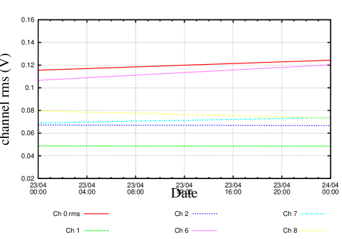
Figure 34: Corresponding rms voltages of channels plotted in previous figure. Color scheme identical to previous plot.

III.3.1 TDC performance and stability

We know that the TDC hit time in unbiased events should roughly correspond to the signal propagation time through the full DAQ (dominated by the delay board), or approximately 1.4 microseconds. Figure 35 presents the recorded TDC times for unbiased events. Although the overwhelming majority of events cluster at the expected time, we do observe occasional deviations from the known expected time, indicative of either TDC noise or ‘stray’ hits.

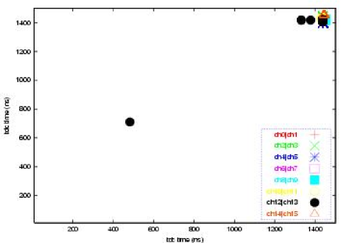
Figure 35: Raw TDC times for the indicated channels, unbiased events. Number of times each channel deviates from 1440 in unbiased evts indicates jitter (bin at (1450,1450) contains 837 events).

III.3.2 Comparison of times recorded by TDC’s vs times derived from waveforms.

A data acquisition system based entirely on fast TDC times would be considerably less expensive, as well as less prone to incurring deadtime. Such a system is effective only if the times extracted from the TDC’s are nearly as reliable as those extracted from waveforms. Unfortunately, it also deprives us of the possibility of imposing matched filtering. Figure 36 shows this correlation for a sample of data. Although largely effective, the large number of off-diagonal entries indicate that the TDC’s are an inadequate proxy for full waveform information.

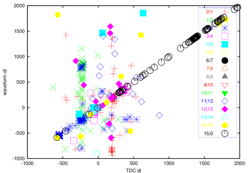
Figure 36: Channel i-channel j hit times, extracted from either raw TDC’s, or waveform times, general events.

III.4 Stability of Full Circuit Gain Calibration

As detailed elsewhere(), KravchenkoB(2003), we have calibrated the total power gain of each receiver to within $\pm$3 dB. In the final step of our amplitude calibration, the antenna response to a calibration signal broadcast from an under-ice transmitter is measured in situ. This test calibrates the combined effects of all cables, signal splitters, amplifiers, etc. in the array. A 1 milliwatt (0 dBm) continuous wave signal is broadcast through the transmit port of an HP8713C NWA. The NWA scans through the frequency range 0$\to$1000 MHz in 1000 bins, at a slow enough sweep rate to ensure that the in-ice amplifiers are not saturated. The signal is transmitted down through $\sim$1000 feet of coaxial cable to one of the five under-ice dipole transmitting antennas. The transmitters subsequently broadcast this signal to the under-ice receiver array, and the return signal power from each of the receivers (after amplification, passing upwards through receiver cable and fed back into the return port of the NWA) is then measured. Using laboratory measurements made at the University of Kansas of: a) the effective height of the dipole antennas, as a function of frequency (previously described), b) the dipole Tx/Rx efficiency as a function of polar angle and azimuth, c) cable losses and dispersive effects (cables are observed to be non-dispersive for the lengths of cable, and over the frequency range used in this experiment), d) the gain of the two stages of amplification as determined from RICE data acquired in situ by normalizing to thermal noise $P_{noise}=kTB=\Sigma_{\omega}<V_{ant}^{2}(\omega)>/Z$, summing over all frequency bins in the bandpass, and e) finally correcting for $1/r^{2}$ spherical spreading of the signal power, one can model the receiver array and calculate the expected signal strength returning to the input port of the network analyzer. This can then be directly compared with actual measurement.

Such a comparison, as a function of frequency, is shown in Figure 37; for each frequency bin, shown is the difference between calculated vs. measured full-circuit gain. Below 200 MHz, the attenuating effect of the high-pass filter is evident. Figure 37 thus shows the deviation between the calculated gain minus the measured gain, for an ensemble of data runs. Included in the Figure are each of the 500 1-MHz bins between 200 MHz and 700 MHz, for three transmitters. I.e., for each frequency bin, we determine a gain deviation and enter that value in the Events vs. Deviation histogram. The average deviation between model and measurement over that frequency range is calculated as $\Delta(G_{calc}-G_{meas})\pm\sigma_{G_{calc}-G_{meas}}$, where $\Delta(G_{calc}-G_{meas})$ is the mean of each of the distributions shown in the Figure, and $\sigma_{G_{calc}-G_{meas}}$ is the error in the mean, given by the r.m.s. of the distribution itself divided by the number of points in each distribution. For the five currently functional transmitters, the mean differences between the expected and the measured gain are $-0.6\pm 0.6$, $-0.8\pm 0.6$, $-2.3\pm 0.5$, $-3.4\pm 0.6$ and $-2.8\pm 0.6$ dB.

Figure 37: Deviation between expected vs. measured Tx$\to$Rx signal power for three transmitters broadcasting to 16 receivers.

Within the “analysis” frequency band of our experiment (200 MHz - 500 MHz), our quoted level of uncertainty in the total receiver circuit power is $\pm$6 dB; this value is commensurate with the width of the gain deviation distributions. On average, however, the calculated gains quoted above are well within these limits. Note that no correction for ice absorption has been made, given the small scale of the array. Nor have corrections been made for possible AMANDA cable “shadowing” in the same ice-hole, which may account for some of the undermeasurement of signal relative to expectation for transmitter 97Tx4. Given a typical transmitter-receiver separation distance of 100 m, an electric field attenuation length of 100 m would result in a shift of $G_{calc}-G_{meas}\sim$8 dB. Although difficult to quantify, our results are consistent with no observable attenuation.

We have investigated the stability of the gain over a three-year period. Figure 38 shows the comparison of the “full-circuit” gain, between 2000 and 2003. The later data are, in fact, slightly higher in amplitude than the older data in the primary passband ($>$200 MHz), and also have a lower-frequency “cut-off” (due to the replacement of the NHP-250 highpass filters by SHP-200 highpass filters for the purposes of making radioglaciological measurements in 2003-04).

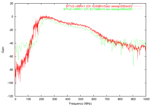
Figure 38: Comparison of network analyzer-derived full circuit gain for $Tx\to Rx$, 2000 vs. 2003.

To calculate eventual upper limits on the neutrino flux, however, we continue to use the more conservative calculated full-circuit gain, from the 2000 data.

III.5 Hit Pattern Recognition

III.5.1 Timing Uncertainties

We have performed an embedding study to evaluate contributions to hit time resolutions and the relative efficacy of various signal time estimation algorithms. Monte Carlo simulations of neutrino-induced hits are embedded into data unbiased events, and the extracted hit times then compared with then known (true) embedded time. Figures 39 and 40 indicate that hit-recognition uncertainties contribute approximately 5-10 ns to the overall timing resolution, per channel.

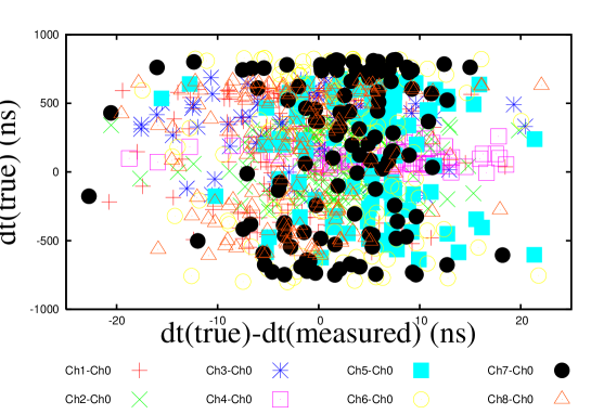
Figure 39: Scatter plot of the difference between the true (embedded) time between antenna hits minus the reconstructed hit time (after embedding) vs. the true time difference. The indicated timing resolution due to pattern recognition uncertainties is approximately 5 ns.

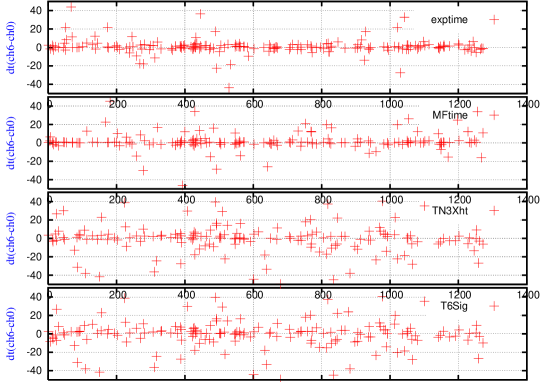
Figure 40: Comparison of the difference between the true (embedded) time between antenna hits minus the reconstructed hit time (after embedding) for 4 different hit time algorithms. The default RICE analysis uses the bottom criterion for hits; the ’exptime’ algorithm, which simply looks for generalized exponential rings, obviously provides superior performance.

III.5.2 Signal Shape Uncertainties

It is obviously essential that, in an experiment such as RICE, we accurately be able to differentiate the hit corresponding to the signal induced in an antenna by a neutrino-generated in-ice shower from background. For a first approximation to what these signals might look like, we used ’thermal noise hits’ drawn from the data itself. Transient ‘hits’ were extracted from a large number of “unbiased” trigger data events. In the offline analysis program, a 34 ns “snippet” of data is saved (10 ns before, and 24 ns after the time-of-maximum voltage, which must exceed 6-sigma) for short-duration transient waveforms having small values of time-over-threshold.

Figure 41 qualitatively indicates the reproducibility of such short-duration transient responses from channel-to-channel (2002 data), with transmitter signal shown in 42 for comparison. These waveforms, channel-by-channel, are used as one of our matched-filter, or ‘transfer function’ templates in future analysis.

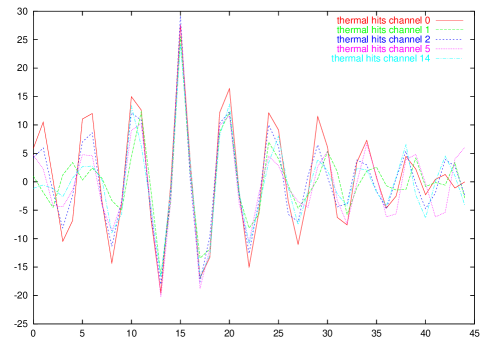
Figure 41: “Short-duration” waveforms, taken from 2002 ‘noise’ data, selecting cases with fast impulsive responses (designated as “thermal hits”), for the indicated channels.

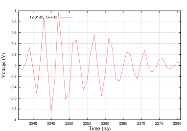
Figure 42: Transmitter data, channel 1, for comparison with ’thermal’ hits.

An additional test of our derived filter is afforded by comparing the signal we observe in transmitter data with simulation of RICE transmitter$\to$receiver signals. Figure 43 shows the comparison between true transmitter data (top, 96Tx1 data) with the expected signal from 96Tx1 in a RICE receiver, using the RICE ‘radiomc’ Monte Carlo simulation code. Although $\omega_{MC}\sim 1.2\omega_{data}$, the general agreement between the two curves is reasonably good.

Figure 43: Receiver time-domain signal resulting from a transmitter broadcasting in the ice, compared with predicted shape.

Qualitatively, the decay time is related to the inverse of the bandwidth – the observed in-ice decay time of $\sim$5-8 ns corresponds to an expected in-ice bandwidth of $\sim$150-200 MHz. The number of cycles in the signal can be, as a general rule, related to the fractional bandwidth: $\Delta f/f_{0}$, with $f_{0}$ the center frequency of the antenna response and $\Delta f$ the bandwidth response (in MHz). For the RICE antennas, based on our effective height curve (Figure 8), we note that: a) the bandwidth is $\sim$300 MHz (which gets down-shifted to $\sim$200 MHz in ice), and b) the fractional bandwidth is about 300 MHz/800 MHz, or 0.3, corresponding to an expectation of 3 cycles in the signal. Cable attenuation reduces the bandwidth somewhat, resulting in an expectation of $\sim$3–4 cycles in the signal.

A knowledge of the expected signal shape allows construction of a ’matched filter’, which provides, in principle, a more precise estimate of the time of a true signal than a simple threshold crossing. Calculation of a simple dot-product between the matched filter vector and the waveform data vector gives a measure of the correlation between putative and true signal shape. A comparison of filters derived from RICE transmitter data, RICE Monte Carlo simulations of neutrino interactions, as well as short-duration transients (“thermal” filters) is shown in Figure 44.

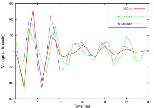
Figure 44: Comparison of filters used in neutrino analysis (Channel 1, 2002 data). Red is Monte Carlo neutrino simulations; green is “thermal hit” matched filter derived from data and blue corresponds to matched filters derived from transmitter data.

Numerically, the filters are implemented by calculating a correlation parameter at each point in the waveform, defined as: ${\bf C}=(\Sigma_{i}F_{i}\cdot(V_{i}-<V>))/\Sigma_{i}|F_{i}|^{2})/\Sigma(F_{i}-(V_{i}-<V>))^{2}$, with $F_{i}$ the $i^{th}$ element of the 34-element filter vector, $<V>$ the average voltage in the waveform ($\equiv$0 in the absence of baseline drifts), and $V_{i}$ the data voltage. The sum is carried out for the 34-elements of our filter arrays. For large amplitude signals which match the shape of the filter, the numerator (generically designated as the ‘Correlation Parameter’ Corrparm, or the “filter dot product”) is large, and the denominator (generically designated as the ‘$\chi^{2}$’) small. The particular value of the cut on this statistic is set by determining the ${\bf C}$ distribution for a large sample of unbiased events, and requiring that the probability of a false positive be less than $10^{-3}$; i.e., that in our sample of unbiased events, less than 0.1% of the waveforms have ${\bf C}>C_{min}$. For 20 waveforms per event, this corresponds to a fake rate of order $<2$%.

Figure 45 illustrates the correlation parameter for a typical waveform.

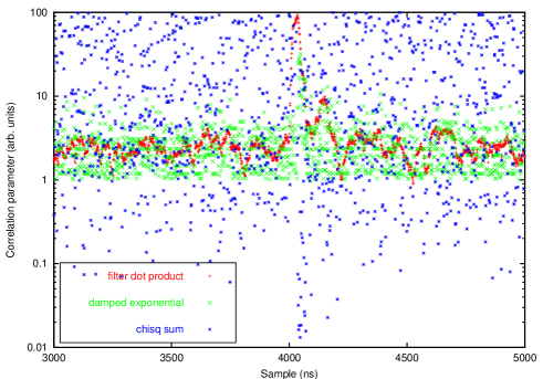
Figure 45: Typical correlation parameters, comparing the value of Corrparm (red points) with the match of a waveform to a general damped exponential form (green points). We have zoomed into the signal region to show greater detail. Also shown is the $\chi^{2}$ value (blue) for the filter. In this event, there was a Monte Carlo signal embedded in an unbiased event at time t=4000 ns in channel 0. The filter used here was the thermal event filter.

Figure 46 shows the agreement in the extracted hit time for a set of general trigger events. Figure 47 shows the agreement in the calculated minimum $\chi^{2}$ and Figure 48 shows both the minimum in $\chi^{2}$ and the maximum in the overall correlation parameter for 10 channels.

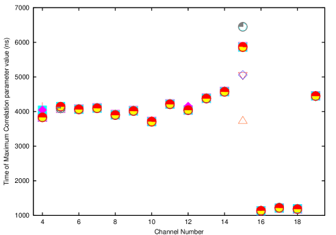
Figure 46: Times of Maximum of correlation parameter for 8 different filters. The filters used are the ‘thermal’ filters, the monte carlo ‘radiomc’ filters, as well as filters derived from data using the five different transmitters broadcasting to the RICE array. We note general consistency in the returned times.

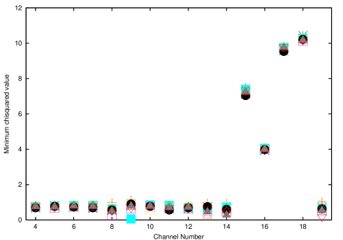
Figure 47: Minimum $\chi^{2}$ at times corresponding to maximum of correlation parameter for 8 different filters.

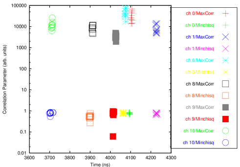
Figure 48: Max Corrparm and Min $\chi^{2}$, and corresponding times in waveform.

In general, the filters give comparable performance. We note that, in our current data analysis, we have used only a threshold-crossing time to define the antenna hit time.

IV Offline Data Filtering

As data are taken, they are collected on the disk of the local PC. Once a day, a script ftp’s the most recent data to a PC (linux), where the first stage of offline analysis occurs, as follows:

1. For each event, each waveform is scanned and we determine (among other things): a) the maximum voltage in the waveform, as well as the time of the maximum voltage, b) the time and voltage of the first, and last 6$\sigma$ excursions in the waveform, c) the rms voltage in each waveform. To minimize the number of scans, the rms calculation is based on the first 500 ns of data in the waveform, which should be far from the trigger-time of $\sim$4$\mu$sec.

2. Once the rms-voltage in each waveform is determined, we can further determine the number of samples for which the waveform exceeds $6\sigma$ (aka “Time-Over-Threshold”, or, simply, “TOT”), in a 2nd scan of the waveform. Based on our knowledge of the transfer function (discussed earlier), this quantity is expected to typically be less than 20 samples for real neutrino events.

At this first stage of event selection, we now require that: a) there be at least 4 channels having $6\sigma$ excursions in the event, and that b) there be no channels having TOT$>$25 ns (the number of total channels with TOT$>$25 ns is designated “NXTOT”). Such cuts should anticipate any possible RICE analyses (GRB’s, wimps, monopoles, air showers, etc.) and be sufficiently general so as to have $\sim$100% efficiency for any such future analyses. We emphasize, however, that all triggers are written to tape and are available for future analysis.

To estimate what inefficiency the Time-Over-Threshold cut would incur for true neutrino events, we consider what fraction of unbiased events would fail the TOT cut, since such unbiased events are expected to constitute the “background” on top of which a true neutrino event would be superposed. For August, 2000 data, the fraction of unbiased events having NXTOT=0 is ($96.0\pm 0.3$)%.

IV.1 Vertex Reconstruction

IV.1.1 Hit-Definition and Gain Stability

As stated above, we require “hits” to exceed the measured rms voltage in each channel at some minimum $N_{\sigma}$ level, with $N\sim 5.5-6$. The $N_{\sigma}$ requirement was selected on the following basis: assuming Gaussian thermal noise, the probability of having an $N\sigma$ excursion on any given sample is: $p_{N}=A\int_{n}^{\infty}exp(-n^{2}/2))$, with the normalization constant $A=1/\sqrt{2\pi}$. For $5.5\sigma$, this corresponds to $p_{5.5}=3.8\times 10^{-8}$. The probability of having at least one such excursion in one of 16 waveforms, each waveform comprising 8192 samples is then (approximately) $p_{5.5}\times 8192\times 16\sim$0.5%. For a 5-sigma criterion, this probability is $\sim$7.5%. In practice, there are non-Gaussian tails in the noise distribution. Figure 49 shows the two-dimensional raw voltage distribution (from which the rms is calculated) for eighteen channels (2002 data).

Figure 49: Distribution of raw voltages for the August, 2000 data, incrementing by channel (along the x-axis). The absolute voltages have all been scaled to a unit normalization, for display purposes.

Figure 50 shows the calculated rms voltages for nine RICE data channels taken from Jan., 2003 vs. June, 2003. Although the former dataset is largely Gaussian, the latter data set shows non-Gaussian tails.

Figure 50: Distribution of rms voltages in nine channels for “unbiased” triggers, taken from Jan., 2003 (solid), and compared with data taken from June, 2003 (dashed). We note the presence of non-Gaussian “tails” in the latter data sample. The difference in widths, from channel-to-channel, are primarily the result of different cable losses in the various channels.

For August, 2000 data, the fraction of the unbiased events having at least one $4\sigma$ excursion is 100%; for $5/6/7\sigma$, the corresponding fractions are 65%, 8.5%, and 5.6%, respectively. Taken at face value, these numbers indicate that, in 8.5% of all neutrino events that might have occurred in august, 2000, there would have been at least one spurious $6\sigma$ hit in the waveform. This requires an event reconstruction algorithm which can robustly identify possibly spurious hits and reject them, based on waveform information (discussed later in this document).

IV.2 Vertexing Studies and In-Ice Transmitter Reconstruction

Beyond the initial filtering discussed in the document, vertex distributions are perhaps the most direct discriminator of surface-generated ($z\sim 0$) vs. non-surface (and therefore, candidates for more interesting processes) events. Consistency between various source reconstruction algorithms is, of course, desirable in giving confidence that the “true” source has been located.

IV.2.1 Application of Matched Filters to Vertexing

Figure 51 shows the z-distribution reconstructed using various codes: top) depth of source vertex obtained using grid algorithm (zgrid), using time of “maximum voltage” in a waveform as the hit time, for all channels; middle) 4-hit source reconstruction algorithm, using same maxVolt criterion as in top plot; bottom) grid-based algorithm, using as the hit time the time when the waveform best matches a “ringing exponential”. We note general agreement between the three depth distributions.

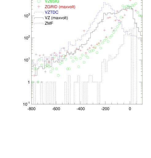
Figure 51: Reconstructed z-vertex for different source reconstruction codes, and for different time-of-hit algorithms, for 80% of the full 2000 dataset.

The smaller statistics for the last matched filter distribution is a consequence of the smaller fraction of times the filter finds 4 hits.

Figure 52 shows the x-y projection of found vertices (grid-vertex-finder) for general triggers in the August, 2000 data, for which there are 10 or more receivers hit in the event. The main “cluster” is consistent with MAPO. The ‘reflection’ in the upper left results from the case where one of the shallow receivers in the northwest corner of the grid registers a spurious, early hit, which pulls the vertex in that direction. This cluster can be suppressed with increasingly stringent hit definitions.

Figure 52: Distribution of xgrid vs. ygrid, August, 2000 general events. In making this distribution, we have required a high hit multiplicity (NHIT$\geq$10).

IV.2.2 Time Residual Studies

An additional discriminant of “well-reconstructed” vs. “poorly-reconstructed” sources is provided by calculating the average time residual per hit. This is done by: 1) finding the most-likely vertex for the event, 2) calculating the expected recorded hit time, for each channel, assuming that vertex. This is a combination of ice-propagation time plus cable delays plus electronics propagation delays at the surface. 3) calculating the difference between the expected time minus the actual, measured time, for that reconstructed vertex (this is, in fact, the same parameter which, when minimized, defines the reconstructed vertex, using the grid-based algorithm). That time difference is defined as the “time residual” (as defined for fits to the helical trajectory expected for a charged track traversing a multi-layer drift chamber).

On a more fundamental level, it is necessary that the overall channel-to-channel timing calibration be performed satisfactorily, and that the timing delays channel-to-channel, within the DAQ, are known, if we are to confidently perform source vertexing. The initial timing calibration is done with simple TDR (Time Domain Reflectometry) measurements at the Pole, for which a signal is sent to each antenna, and the time delay between the SEND signal and the reception of the RETURN signal divided by two gives the one-way transit time delay. If all the system delays are known, then (as mentioned previously), time residuals should be zero for perfectly fit vertices.

Figure 53 shows the scatter plot of the average time residual, per channel, vs. the number of 6-sigma excursions in an event, comparing all general triggers (August, 2000 data) with the subset of those triggers having NXTOT=0. We note two features of this scatter plot: 1) as expected, the events which have NXTOT=0 favor lower hit multiplicities - i.e., the more channels that are ON, the more chances to have one channel fail the $TOT<$25 ns cut, 2) as N6SIG increases, the time residual per hit does, in fact, decrease, indicating a better-reconstructed vertex.

Figure 53: Time-residual per hit antenna (in units of ns, horizontal) vs. the total number of 6-sigma excursions (vertical). The open squares show the distribution for all general triggers; the filled in circles show the distribution for general triggers having NXTOT=0.

To corroborate that conclusion, Figure 54 shows the distribution of time residual per hit channel (ns) vs. the depth of the reconstructed vertex (vertical). Open squares are general triggers, Aug. 2000 data. Filled-in squares correspond to 97Tx3 pulser data, taken January, 2001. We note that: a) the time-residual per channel for pulser data clusters at very small values, b) there is very little scatter in the reconstructed depth for the 97Tx3 pulser data, c) the cluster of events corresponding to $zgrid\to$0 occurs predominantly for small values of $<\delta t>$. Such a goodness-of-vertex cut can be used to select well-fit vertices.

Figure 54: Average time residual (“$<\delta t>$”) per hit (horizontally, in units of ns) vs. location of reconstructed vertex (vertical, units are meters) for August, 2000 data vs. 97Tx3 pulser data (from 2001).

Following Figure 54, Figure 55 presents channel-by-channel time residuals for August, 2000 general events (black), compared to time residuals for 97Tx3 pulser data (the same data that were used for comparison purposes in Figure 54). Typical channel-to-channel time residuals are of order $<$10 ns for the 97Tx3 pulser data (shown in red).

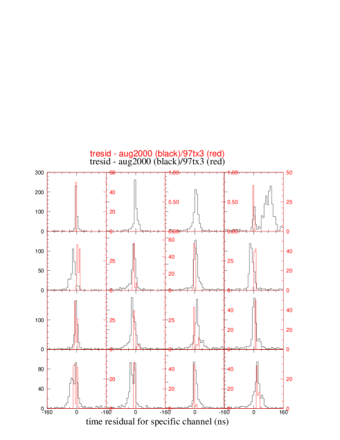
Figure 55: Time residual, channel-by-channel, for general triggers, August, 2000 data (shown in black) compared to pulser data (97Tx3). Note that the 97Tx3 transmitter is in the same hole as the channel 3 receiver; transmitter receiver coupling effects ‘contaminate’ the waveform and therefore bias the reconstructed hit time. Horizontal axis is time residual, in units of nanoseconds. Top row channels are, left to right: 0, 1, 2, 3. Second row: 4, 5, 6, 7 (etc.)

By contrast, for the August, 2000 general events (shown in black), distributions are considerably wider.

For a perfectly fit vertex, the time residuals are all zero. Additional transmitter data are shown in Figure 56, for samples of transmitter data taken in January, 2003. Figures such as these can be used to determine an average timing correction, channel-by-channel, based on information from all transmitters.

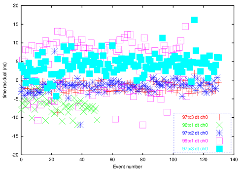
Figure 56: Channel 0 time residuals, for five different transmitters, showing typical channel timing calibration and response.

Based on the observed channel-per-channel average time residuals, we can derive a 2nd-order correction to the channel-by-channel time delays derived from time-domain-reflectometer measurements. These 2nd-order timing offsets are shown in Figure 57. The points are derived from the same data set used to measure n(z) in a previous publication ((), Kravchenko(2004)).

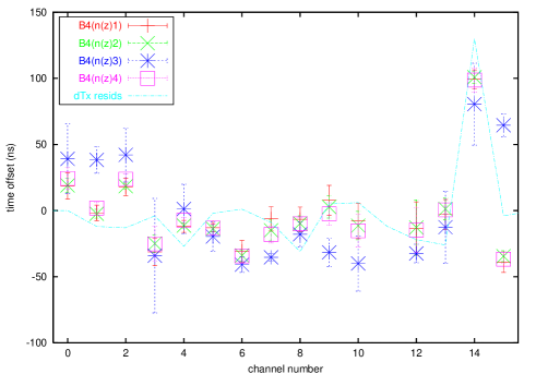
Figure 57: Timing offsets derived from B4 data vs. tx data.

The sum of the timing residuals, for any putative event vertex, gives us a value of chi-squared, which, when minimized, defines the ’grid’-vertex. The shallowness of the chi-squared distribution, indicating the typical uncertainty in the reconstructed vertex, is shown for two typical events in Figures 58 and 59. The minimum is observed to be fairly broad, corresponding to a typical uncertainty (statistical) within the center of the array of order tens of meters.

Figure 58: Chi-squared contour, using grid-based vertexing algorithm, of a typical “general” trigger; data taken from 2000 sample (Day 88, event 103). Shown is the $\chi^{2}$, in units of $ns^{2}$, around the selected vertex. Displayed is only the vertex in x-y.

Figure 59: Chi-squared contour, using grid-based vertexing algorithm, of a typical transmitter event; data taken from 2001 sample (Day 2, event 1). Shown is the $\chi^{2}$, in units of $ns^{2}$, around the selected vertex. Displayed is only the vertex in x-y.

IV.2.3 Spatial Residuals

The spatial residuals are correlated with, but also provide somewhat independent information relative to the time residuals. To investigate the possibility of incorrect spatial pulls of any one channel on the event reconstruction, Figures 60, 61, and 62 are derived from the 4-hit ‘analytic’ fitting algorithm, as follows: for each event, having hit multiplicity $N$, for which $N>$4, one makes 4-hit subsets of the total $N$ hits and vertexes using those 4-hit subsets. At the end of calculating all the possible vertices, one constructs an “average”, or “best”-vertex, which is then reported back to the user. One can compare the vertex calculated from those subsets including channel $i$ with the vertex calculated from those subsets excluding channel $i$. If the timing calibration has been performed properly, and if the surveyed locations of all the receivers have also been recorded properly, the two sets of calculated vertices (the set based on 4-fold combinations including channel $i$ vs. the set based on 4-fold combinations excluding channel $i$) should coincide with each other. We show the difference between those two vertices, in the x-coordinate (Figure 60), y-coordinate (Figure 61), and z-coordinate (Figure 62), respectively, scatter plotted against the reconstructed depth of the vertex (the vertical coordinate in each of these plots) for the August, 2000 data. Calibration constants giving corrections to the surveyed locations of the receivers (in particular, for channel 3 and channel 10) are based on distributions such as these.

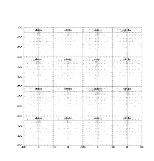
Figure 60: Difference between x-coordinate of the vertex calculated including the indicated channel minus x-vertex calculated excluding the indicated channel (horizontal), obtained from the 4-hit algorithm, vs. reconstructed vertex depth (vertical), for August, 2000 data. Units are meters.

Figure 61: Difference between y-coordinate of the vertex calculated including the indicated channel minus y-vertex calculated excluding the indicated channel (horizontal), obtained from the 4-hit algorithm, vs. reconstructed vertex depth (vertical), for August, 2000 data.

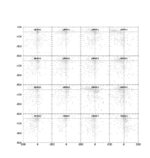
Figure 62: Difference between z-coordinate of the vertex calculated including the indicated channel minus z-vertex calculated excluding the indicated channel (horizontal), obtained from the 4-hit algorithm, vs. reconstructed vertex depth (vertical), for August, 2000 data.

Figures 63, 64, and 65, which show the corresponding plots for 97Tx3 data, are obtained using the timing-derived calibration constants. We note that, for surface source locations, ray tracing must be performed through the firn to the surface. Even after application of ray-tracing corrections, we note that a large fraction of the solid angle above the surface is folded into caustics around the total internal reflection angle, which makes unique identification of a surface source difficult if it is not directly over the array. For sources such as 97Tx3 (and, in general, for $z<-150$m, which corresponds to the neutrino search region), such corrections are less important, although still non-zero for shallow receivers.

Figure 63: x-spatial residual: Difference between x-coordinate of the vertex calculated including the indicated channel minus x-vertex calculated excluding the indicated channel (horizontal), obtained from the 4-hit algorithm, vs. reconstructed vertex depth (vertical), for January, 2001 pulser data. The large apparent error in the Channel 2 receiver (top row, 3rd column) results from the transmitter being pulsed being in the same hole as that receiver.

Figure 64: y-spatial residual: Difference between y-coordinate of the vertex calculated including the indicated channel minus y-vertex calculated excluding the indicated channel (horizontal), obtained from the 4-hit algorithm, vs. reconstructed vertex depth (vertical), for January, 2001 pulser data. The large apparent error in the Channel 2 (top row, 3rd column) receiver results from the transmitter being pulsed being in the same hole as that receiver.

Figure 65: z-spatial residual: Difference between z-coordinate of the vertex calculated including the indicated channel minus z-vertex calculated excluding the indicated channel (horizontal), obtained from the 4-hit algorithm, vs. reconstructed vertex depth (vertical), for January, 2001 pulser data.

V Further consideration of physics backgrounds

V.1 Detectability of cosmic ray muons in RICE

Several processes can, in principle, contribute to the actual muon event rate expected in RICE. These include: contributions from the Coulomb field of muons passing close to a RICE radio receiver. For vertical muons passing near two vertically displaced receivers, the signature is, in principle, clean - two hit times separated by t=d/c rather than t=d/(c/n). Pictorally, the transverse field increases by $\gamma$, whereas the longitudinal field (to which we are sensitive for downcoming muons) is invariant. (In frequency space, the vertical extent of a typical RICE dipole sets the scale of the bandwidth response. Although the field lines are Lorentz-contracted, the Lorentz free space contracted time scale is $\sim\gamma$ smaller, and the bandwidth is $\sim\gamma$ larger, so $\gamma_{net}\sim$1.) Therefore, there is a maximal mismatch of geometries – for the predominantly vertical muon flux, the vertically-oriented dipoles are most sensitive to the (unboosted) longitudinal component of the Coulomb field.

Nevertheless, we can estimate the field strengths, for, e.g., vertically-incident flux. Neglecting effects due to the Lorentz contraction of the field lines, zt a distance of one meter from an antenna, $V\sim(q/(4\pi\epsilon_{0}r^{2}))\times h_{eff}$, or approximately 0.144 nV – roughly 5 orders of magnitude smaller than the mean rms thermal noise. We therefore require $\gamma\sim 10^{5}$, or $E_{\mu}\sim 10^{13}$ eV, with the greatest sensitivity to horizontal muons (unfortunately, the muon flux $dN/d\theta\sim sec\theta$). We can search for events by looking for signals in multiple channels having a transit time between channels corresponding to motion of an ultra-relativistic charged particle. Figure 66 shows no obvious band corresponding to a particle moving through the ice at v=c.

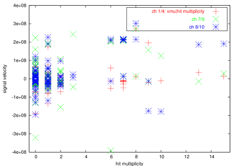
Figure 66: Propagation velocity for signals registered in two receivers in same icehole, for non-general triggers, data taken 10Dec03. No obvious band at v=c is observed.

V.1.1 Muon Bremstrahlung

We have written a crude simulation to estimate the expected signal from possible muon bremstrahlung. GEANT simulations of muons passing through ice allow us to investigate the expected increase in the bremstrahlung cross-section with muon energy. (Note that the GEANT estimates do not include the enhancements in the muon observability due to photonuclear interactions, which become dominant at energies greater than 100 EeV(), Klein(2004).) Figure 67 shows the correlation of mean-free-path (distance between successive bremstrahlungs) and fraction of energy lost in a bremstrahlung for three different muon energy ranges. At each bremstrahlung, we calculate the expected signal voltage induced in a receiver antenna, assuming $V_{eff}\sim 0.1$m, and using the original ZHS(), Zas(2006) estimate of the signal strength on the Cherenkov cone. This is then compared with the rms thermal noise voltage $V_{thermal}=kTB$.

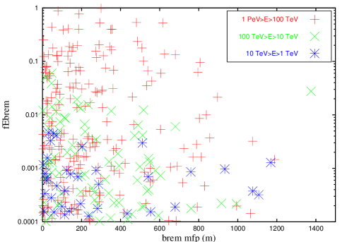
Figure 67: Fraction of muon energy lost to bremstrahlung, as a function of muon energy, using GEANT simulations.

For this simulation, we generate the muon flux on the ground, as given by Gelmini, Gondolo and Varieschi(), Gelmini(2002) which includes both muons from high energy primaries, as well as muons from charm produced by cosmic ray interactions in the atmosphere. We model these two contributions using the prescription in the Review of Particle Properties(), RPP(2006): $dN_{\mu}/dE$(conventional)$\sim(0.14E^{-2.7})$*((1/(1+((1.1E)/115))) + (0.054/(1+((1.1E)/850)); (E in GeV, flux in $GeV^{-1}s^{-1}sr^{-1}$). The charm flux, as presribed by GGR, is modeled as a simple power law, with a vertical component which is approximately $E^{0.5}$ harder than the conventional flux, and crosses the conventional flux at approximately 1 PeV.

Figure 68: Signal distribution expected from muon bremstrahlungs in one year.

The expected signals induced by bremstrahlungs, in one year, are shown in Figure 68. (Multiple y-values for the same x-value correspond to multiple receivers hit for the same muon). We note that there are no signals which exceed a value of S:N$\geq$1. The trigger efficiency of such signals is, in principle, enhanced by writing to disk all events for which there is a coincidence between a high-multiplicity SPASE (South Pole Air Shower Experiment) event and a hit RICE receiver. The timing delay between the expected RICE signal and the expected SPASE trigger time received at the RICE DAQ is shown in Figure 69, taking into account known cable delays, etc. Given the timing coincidence of 1.25$\mu$sec, we should have adequate efficiency for detection of bremstrahlungs, in the event that the signal were sufficiently large. However, as shown in the Figure, our timing delays are, in fact, not tuned to match the expected delay between the SPASE and RICE triggers.

We point out that this timing correlation estimate is, admittedly, extremely crude – in a realistic scenario, an air shower would probably produce multiple muons, one of which would trigger the DAQ early, and a later one of which would trigger RICE (we also have only very crudely estimated the details of the SPASE trigger, with which we have very limited familiarity).

Figure 69: Expected timing correlations between RICE and SPASE hits due to single muons.

We have separated our events by trigger type, and reconstructed corresponding event vertices. As shown in Figure 70, the xy-location of the reconstructed vertex is, in fact, different for the various trigger types - perhaps most interestingly, the SPASE coincidences show a marked shift, in the direction of the SPASE array, relative to ‘general’ triggers (which are consistent with the sub-sample of veto triggers that are saved to disk). A full analysis of these triggers has, however, not yet been conducted.

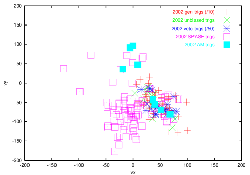
Figure 70: Vertex distributions for various trigger types, xy-projection. “Veto” triggers are triggers identified as likely of surface origin, based on fast timing (TDC) information. “General” triggers are multiplicity 4 events which have not been identified as “veto” events. “Unbiased” triggers correspond to data captures taken at random times, “AM” and “SPASE” refer to coincidences between AMANDA-B triggers or SPASE triggers, to within 1.25 microseconds.

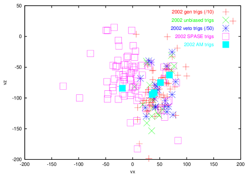
Figure 71: Vertex distributions for various trigger types, yz-projection. Scheme is the same as in the previous Figure.

In principle, timing correlations between receivers, in the case of a “muon bundle”, e.g., might be used to accentuate the possible signal – in this case, one takes advantage of the fact that the muon bundle is propagating at the velocity of light while Cherenkov radiation, e.g., will propagate at $v\sim 0.6c$. This has not yet been fully investigated.

V.2 Air Shower Backgrounds

Direct radiofrequency signals from extensive air showers (EAS) which propagate into the ice, as measured by the CODALEMA and LOPES experiments, give signals which peak in the tens of MHz regime. There should be a signal resulting from the impact of the shower core with the ice, producing the same kind of Cherenkov radiation signal that RICE seeks to measure. Nevertheless (Fig. 72), the expected EAS signal rate should be almost immeasurably small.

Figure 72: Estimated EAS detections per year for RICE and ANITA.

V.3 Solar RF Backgrounds

Radio frequency noise correlated with solar activity has been the subject of extensive investigation. Auroral discharges have been continuously monitored in Antarctica in the tens of MHz frequency range, over the last decade. In 2003, there were high-intensity solar flares recorded between Oct. 19, 2003 to Nov. 4, 2003; typically, these result in electrical disturbances at Earth some 24-48 hours later. We have looked for correlations, during this time period, with high backgrounds as registered by RICE (based on low livetime, or, alternately, high discriminator thresholds needed to maintain reasonable livetimes). Figure 73 shows these quantites, as monitored through this time period. No obvious correlation is observed.

Figure 73: LiveTime (crosses) and also discriminator thresholds (in Volts) for days 280 – 310 of 2003. Solar flares were registered on Oct. 31 (registered at Earth at 9:54 am UT) and Nov. 6 (7:20 am UT), corresponding to Julian days 304/305 and 310/311.

V.4 Correlation with Machine Activity at South Pole Station

We have searched for correlations with aircraft activity at Pole, but find no obvious correlation. Nevertheless, operating machinery (in particular, the IceCube drill) creates large amplitude backgrounds that render our data-taking during the austral summer largely ineffective. Fortunately, conditions during the austral winter tend to be generally radio-quiet.

VI Future Running

The current RICE data-taking is expected to continue for the next 3-4 years, yielding an incremental improvement in sensitivity largely proportional to the increase in livetime. A second-generation experiment would address: 1) the limited bandwidth of the experiment, resulting from cable losses at high frequencies, the need to highpass filter above 250 MHz in order to reduce low-frequency noise from the AMANDA (and later, IceCube) phototubes, and the 500 MHz bandwidth of the digital oscilloscopes, and 2) the high thresholds resulting from a simple one-tier trigger system and the inability to effectively reduce surface backgrounds in hardware. We are currently developing a successor to the present RICE array (“AURA”), featuring in-ice custom digitizer boards, and a local coincidence multiplicity trigger, which only considers “hits” for which a local antenna cluster (consisting of 4 antenna) itself satisfies a local trigger coincidence inconsistent with down-coming signals.

In the IceCube era, we hope to expand the capabilities of RICE with improvements to both the receiver modules as well as the data acquisition system. A sketch of the future array is outlined in Figure 74. We anticipate in-ice sampling, and transmission of digital signals to the central Counting House, where the event trigger is formed and digitization occurs. Vertically, there are two “close” clusters, both below the firn, and one deep cluster. Assuming no dedicated ice-hole drilling and only co-deployment with IceCube, we show the horizontal footprint expected in the “IceCube-Plus” scenario. The in-ice antennas are complemented by downward-looking surface horn antennas, which view only upcoming signals (and obviate in-ice deployment issues) and also are necessary for ensuring the maximal rejection of down-coming noise. Local “clusters” allow suppression of spurious randoms and also ensure that recorded signals are up-coming rather than down-going. Figure 75 illustrates the geometry of a possible RICE-IceCube overlap event.

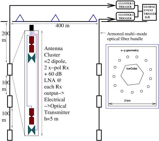
Figure 74: RICE-II schematic.

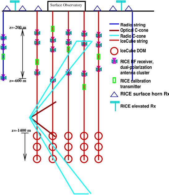
Figure 75: Geometry of ICECUBE - RICE event.

Monte Carlo array optimization studies are in progress. Figures 76, 77, and 78 show the expected sensitive volume of a neutrino array, and its dependence on the array geometry and spacing between array elements. In general, the most efficient array studied is a shallow array (filling the depth region between –200 m and –600 m) with typical horizontal spacing of $\sim$1 km and typical vertical spacing of $\sim$100 m, reflecting the typical scale of the attenuation length, and the width of the Cherenkov cone for a typical neutrino interaction, respectively.

Figure 76: Neutrino Effective volume, as a function of depth of array.

Figure 77: Neutrino Effective volume, as a function of the surface extent of the array.

Figure 78: Neutrino Effective volume, as a function of vertical spacing of the array.

Expected performance is also being evaluated. Figure 79 displays the effective volume dependence on the minimum required event multiplicity.

Figure 79: Neutrino Effective volume, as a function of minimum “event” multiplicity required.

Figure 80 illustrates that relatively large timing uncertainties are tolerable if the array is distributed over a large area.

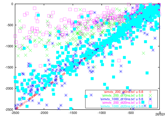
Figure 80: Generated (horizontal) vs. reconstructed source depth, for various configurations of antennas and timing resolutions. Perfect source reconstruction results in a narrow band along the diagonal.

One of the most important experimental factors determining signal detection rates is the center frequency of the antenna, and how that relates to the bandwidth of noise (and the S:N for true neutrinos); the S:N rate is what then dictates the appropriate operating discrimator threshold.

Figure 81: Relative signal yield as a function of discriminator threshold and center frequency of antennas.

A multiparameter optimization and expected event rates for various experimental configurations has been ongoing, and will continue as our understanding of such things as ice properties improve and practical limitations such as drilling costs and overhead become better-defined.

VII Acknowledgments

The RICE experiment is supported by NSF Office of Polar Programs Award No. 0338219, the University of Kansas, and the Research Corporation. We thank our RICE colleagues for making the experiment possible.

References

- (1) Kravchenko et. al., Astropart.Phys. 20 (2003) 195-213
- (2) Kravchenko et. al., Astropart.Phys. 19 (2003) 15-36
- (3) Kravchenko et. al., J. Glac., vol 50, no. 171, (2004) 522-532
- (4) S. Hussain and D. McKay, Phys.Lett. B634 (2006) 130-136
- (5) Kravchenko et. al., Phys.Rev. D73 (2006) 082002
- (6) Besson et. al., Astropart.Phys. 26 (2007) 367-377
- (7) Zas, Halzen and Stanev, Phys. Rev. D 45, 362 (1992)
- (8) Alvarez-Muniz et. al., Phys.Rev. D74 (2006) 023007, and references cited therein.
- (9) S. Razzaque et. al., Phys.Rev. D70 (2004) 103003, and references cited therein.
- (10) Butkevich, Dedenko and Provorov, The SIMEX simulation package, (unpublished).
- (11) Buniy and Ralston, Phys. Rev. D 65, 016003 (2002).
- (12) www.farr-research.com/Papers/ssn426.pdf
- (13) arXiv:astro-ph/0412546
- (14) arXiv:hep-ph/0209111
- (15) Review of Particle Properties, pdg.lbl.gov