Matching WMAP 3-yrs results with the Cosmological Slingshot Primordial Spectrum

Abstract

We consider a recently proposed scenario for the generation of primordial cosmological perturbations, the so called Cosmological Slingshot scenario. We firstly obtain a general expression for the Slingshot primordial power spectrum which extends previous results by including a blue pre-bounce residual contribution at large scales. Starting from this expression we numerically compute the CMB temperature and polarization power spectra arising from the Slingshot scenario and show that they excellently match the standard WMAP 3-years best-fit results. In particular, if the residual blue spectrum is far above the largest WMAP observed scale, the Slingshot primordial spectrum fits the data well by only fixing its amplitude and spectral index at the pivot scale $k_{p}=10^{-3}h\mbox{Mpc}^{-1}$. We finally show that all possible distinctive Slingshot signatures in the CMB power spectra are confined to very low multipoles and thus very hard to detect due to large cosmic variance dominated error bars at these scales.

SISSA 37/2007/A; DAMTP-2007-50

1 Introduction

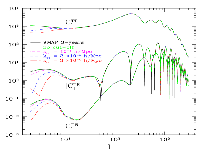
Figure 1: Temperature and polarization CMB power spectra in the slingshot scenario, compared to the standard WMAP 3-years best-fit cosmological model. The cosmological parameters $\Omega_{b}h^{2}=0.02218$, $\Omega_{c}h^{2}=0.1010$, $\Omega_{\Lambda}=0.77$, $\tau=0.09$, $h=0.74$ are the same in the two model. The primordial spectral index in the standard scenario has been chosen as $n=0.95$, while the slingshot primordial power spectrum is described in section II. The slingshot power spectrum normalization is chosen in order to match the amplitude of the CMB angular power spectrum at $\ell=100$ obtaining $k_{0}=8.86648\times 10^{-7}\ h\mbox{Mpc}^{-1}$. We consider several different cut-off scales and $B\ll\bar{B}$ (see text for further details).

It is well known that Standard (non-inflationary) Cosmology is afflicted by three severe problems KolbTurner : homogeneity, isotropy and flatness. Inflation is the standard accepted paradigm for the resolution of these problems. Nevertheless, as a fundamental origin of Inflation is as yet lacking, many attempts to alternatively solve the homogeneity, isotropy and flatness fine tunings have been recently put forward.

In this paper we consider one of these alternatives, namely the scenario developed in sling ; sling2 so called the “Cosmological Slingshot Scenario”, or shortly the Slingshot.

In the Slingshot, our Universe is a probe $D3$-brane “orbiting” with an open trajectory in a IIB supergravity background, namely the Klebanov-Tseytlin (KT) metric KT (the bulk). If the probe brane approach of kehagias used in sling ; sling2 can be used, the Slingshot trajectory results on an induced cosmological evolution on the brane. More precisely, a brane observer experiences a Friedman-Robertson-Walker non-singular bouncing universe. In the Slingshot, the problems that afflict standard cosmology are circumvented sling by using similar mechanisms introduced in pre big-bang veneziano and cyclic turok scenarios. Besides, the Slingshot also predict a power spectrum of primordial perturbations. In sling ; sling2 , and in this letter, the primordial spectrum of scalar perturbations due to the fluctuation of the Slingshot brane on the KT background is indeed calculated under the approximation that the backreaction of the Slingshot brane into the bulk is negligible. The validity of this approximation is supported by the fact that the KT background, in which the Slingshot brane is moving, is produced by a large number of D3-branes having all the same tension (“mass”) as the Slingshot brane.

The plan of the paper is as follows. In section 2 we will summarize the previous results of sling ; sling2 . We will then extend those results in two ways. First of all we will consider a new blue contribution to the primordial power spectrum that was previously not accounted for. This will produce the general parametrization of the Slingshot primordial spectrum shown at the end of section 3.

As a second step, in section 4, we will use this general parametrization in order to numerically compute the temperature and polarization CMB angular power spectra arising from the Slingshot and we will compare them to WMAP data wmap . In particular we will show that a suitable and natural choice of the Slingshot parameters allow to reproduce the standard WMAP 3-years best-fit power spectra. We will then try different choices for the Slingshot parameters and see if they can produce distinctive model-dependent signatures in the results. Finally we will draw our conclusions in section 5.

We are now ready to conclude this section, but we would like to make a final remark first. In sling2 an analytic expansion of the Slingshot spectrum for large multipoles ($\ell>10$) had actually already been shown to match the WMAP best fit of a power law spectrum with spectral index $n_{s}\simeq 0.95$. However this result held only at a given pivot scale (chosen as $k_{p}\sim 10^{-3}h\mbox{Mpc}^{-1}$). Our numerical approach in this paper shows instead that the spectrum found in sling2 , matches the WMAP experimental results at all scales, and not only around the pivot scale. This is not an obvious result as the Slingshot primordial spectrum presents a non-trivial running of the spectral index.

2 The Original Slingshot Power Spectrum

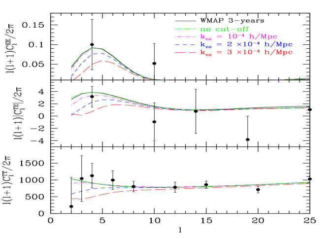
Figure 2: Comparison between WMAP data and low CMB multipoles for different values of $k_{cut-off}$ and fixed $B\ll\bar{B}$ in the Slingshot scenario.

The Slingshot power spectrum of scalar perturbations is related to the quantum fluctuation of the Slingshot $D3$-brane. The way of producing this perturbation is similar to the one introduced by wald but without the drawbacks outlined by muk (see sling2 ). The fluctuation of the brane is of quantum origin and it is in a pure state whenever the comoving wave length of the perturbation is below a fundamental quantum length $l_{c}$. This fundamental length can be consistently chosen to be the first massive mode of the fundamental String or the M-theory minimal length.

During the pre-bounce phase of the Slingshot, the perturbations created in the far past (in the Bunch-Davis vacuum), eventually come back to their vacuum state whenever their wavelength $\lambda=a/k<l_{c}$, where $k$ is the wave number of the fourier mode associated with the wavelength $\lambda$ and $a$ is the scale factor of the induced cosmology on the brane. Viceversa, as the brane re-expands, the wavelength of a given perturbation will grow again. It is therefore clear that after some time, the perturbation wavelength will reach the scale $l_{c}$. At this point the perturbation collapses into its classical state becoming a coherent state as the perturbation is over-damped by the Universe expansion Liddle . After waiting enough time, a stochastic background of primordial perturbations is therefore dynamically (and continuously) created. The distribution of these perturbations is gaussian with variance set by the quantum correlations during the quantum to classical transition. However, since the Slingshot Scenario represent a bouncing cosmology, not all the wavelength of primordial perturbations can be produced with this mechanism. In fact the maximal wavelength that can be produced is

$$\lambda_{\mbox{\tiny cut-off}}=\frac{a_{b}}{k_{\mbox{\tiny cut-off}}}=l_{c}\ ,$$ (1)

where $a_{b}$ is the size of the scale factor at the bouncing. This obviously creates a natural cut-off on the power spectrum.

A remark here is due. The physical process we have just discussed has been developed in the String frame. There, at zeroth order on the brane velocities sling2 , the gravitational coupling is running ($G_{N}\sim a^{2}$) and particle masses are fixed. The Einstein frame, in which the the gravitational coupling is constant, can be then easily obtained by re-scaling the metric by $a^{-2}$. At the background level then, the spacetime in Einstein frame is Minkowski and all particle masses run (note that also the matter Lagrangian is re-scaled). It is therefore easy to convince ourselves that any physical quantity in the two frames is completely equivalent (see faraoni for a general discussion and sling2 for the Slingshot case). Let us however comment the special case of the perturbation spectrum. In String frame the perturbed metric is $ds^{2}_{S}=a^{2}(1+2\Psi)dt^{2}+...$ where $\Psi$ is the Bardeen potential. By re-scaling to the Einstein frame such that $ds^{2}_{E}=(1+2\Psi)dt^{2}+...$, we still obtain the same Bardeen potential $\Psi$. The power spectrum of primordial perturbations (a physical quantity) is therefore unchanged by the change of conformal frames. However, one might still be puzzled whether the String frame cut-off on the perturbations spectrum is still there in the Einstein frame. In the Einstein frame the wavelength of a perturbation is constant in time, i.e. $\lambda=1/k$. However, the quantum length in this frame is re-scaled, together with any other physical length, by a factor $a^{-1}$. In the Einstein frame the quantum length is therefore “bouncing”. This produces, in the Einstein frame, the same cut-off as observed in the String frame.

In sling2 , the Slingshot primordial power spectrum is calculated to be

$$P_{\mbox{\tiny red}}(k)=\frac{A}{k}e^{\frac{1}{2}W_{-1}\left(-\frac{k_{0}^{4}}{k^{4}}\right)}\left[1-e^{\frac{1}{2}\Delta(k_{0}/k;k_{\mbox{\tiny cut-off}})}\right]\ ,$$ (2)

where $W_{-1}$ is the Lambert W function in the real branch $-1$ (see WW for a description of the Lambert function properties), $A$ is an overall normalization of the spectrum and finally $k_{0}$ is a parameter defining the spectral index at large $k$s.

The cut-off function $\Delta(k_{0}/k;k_{\mbox{\tiny cut-off}})$ is defined as

$$\Delta(k_{0}/k;k_{\mbox{\tiny cut-off}})=W_{-1}\left(-\frac{k_{0}^{4}}{k^{4}}\right)-W_{-1}\left(-\frac{k_{0}^{4}}{k_{\mbox{\tiny cut-off}}^{4}}\right)\ ,$$ (3)

where $k_{\mbox{\tiny cut-off}}$ fixes the cut off as $P_{k}$ is positive definite. If the ratio $k_{0}/k$ is small we have $W_{-1}(-k_{0}^{4}/k^{4})\simeq 4\ln(k_{0}/k)$. Therefore for large wave number (i.e. small scales)

$$e^{\frac{1}{2}W_{-1}\left(-\frac{k_{0}^{4}}{k^{4}}\right)}\simeq\frac{k_{0}^{2}}{k^{2}}\ .$$ (4)

In this limit $e^{\frac{1}{2}\Delta}\ll 1$ and the spectrum looks scale invariant.

In order to match the best WMAP fit of a power law power spectrum, following sling2 , we fixed the spectral index of the Slingshot to be $n_{s}=d\ln k^{3}P(k)/d\ln k+1=0.95$ at the pivot scale $\ell=100$. If we neglect the correction due to the cut-off scale, this fixes the parameter $k_{0}$ to be $k_{0}=8.86648\times 10^{-7}\ h\mbox{Mpc}^{-1}$. This parameter is much smaller than any wave number we are going to consider. We can then use the analytical properties of the Lambert W function $W_{-1}(-x)\simeq\ln(x)-\ln(-\ln(x))$, to find the approximate spectrum

$$P_{\mbox{\tiny red}}(k)\simeq\frac{A}{k^{3}\sqrt{\ln\frac{k}{k_{0}}}}\left[1-\frac{k_{\mbox{\tiny cut-off}}^{2}}{k^{2}}\sqrt{\frac{\ln\frac{k_{\mbox{\tiny cut-off}}}{k_{0}}}{\ln\frac{k}{k_{0}}}}\right]\ .$$ (5)

This completes the description of the previous results obtained in sling ; sling2 . In the following section we are going to consider an additional contribution to the Slingshot primordial power spectrum that was not kept into account in previous works.

3 A blue pre-bounce residual

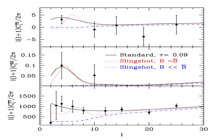
Figure 3: We compare different values of the low-$\ell$ spectrum normalization $B$ for a given value of $\ell_{cut-off}\sim 10$ and optical depth to last scattering $\tau=0.09$. The solid black line represents the standard WMAP 3-years best-fit power spectrum while the dashed blue and dotted redlines are the Slingshot power spectra for small and large values of $B$ respectively.

As previously discussed, primordial perturbations are in general present even during the pre-bounce era. These perturbations, corresponds to the quantum fluctuation of the Slingshot brane during its motion down the throat of the CY. The induced Bardeen potential $\Phi$ evolves with the angular brane motion and its perturbations, as discussed in sling2 . Nevertheless, we can use the approximations used in sling where the Bardeen potential results decoupled from the angular brane motion.

In this case, $\Phi$, follows schematically the Mukhanov equation sling

$$\delta r^{\prime\prime}+\left(k^{2}-\frac{J^{2}}{r^{4}}\right)\delta r=0\ ,$$ (6)

where $r\Phi=\delta r$, $J$ is the brane angular momentum, $r$ parameterize the brane position in the CY throat and finally ^′ is the derivative with respect to the conformal time. $J^{2}/r^{4}$ corresponds to $r^{\prime\prime}/r$. Differently from the inflationary case, however, $r^{\prime\prime}/r$ is not the Hubble horizon.

The induced scale factor of the Universe $a$ is related to $r$ as $a=\frac{r}{L\sqrt{\ln r/r_{s}}}$. $L$ is proportional to the number $N$ of $D3$-branes in the stack and $r_{s}$ is the radius of the blown up sphere at the tip of the CY (see sling for more details). We then see that for $k\gg\frac{J}{r^{2}}$ the system oscillates, particles are not created and the Bardeen potential stays in its vacuum. In the opposite case, $k\ll\frac{J}{r^{2}}$, the system is instead over-damped and eventually $\Phi$ becomes constant. There, particles are created and the system evolves stochastically. In the large $k$ region we therefore have $\langle\Phi(k)\Phi(k^{\prime})\rangle\propto\frac{\delta(k,k^{\prime})}{kr^{2}}$. At the matching point $k=\frac{J}{r^{2}}$, we then have a constant spectrum of perturbations, i.e. a power law spectrum with spectral index $n_{s}=4$. Note that if $J=0$, i.e. for a brane with no-angular momentum, the perturbation is never over-damped and therefore the spectrum will be $P(k)\propto k^{-1}r^{2}$ at any times. In this case the resulting spectral index will be $n_{s}=3$ as found in bran .

These conclusions can also be drawn more precisely by following sling2 and by considering the semi-classical to quantum matching point at $k=Jr^{-2}$.

We then conclude that a blue spectrum of primordial perturbations, coming from the pre-bounce, must be added to the $P_{\mbox{\tiny red}}(k)$. However, this spectrum will survive from being destroyed by the quantum region only for perturbation scales $k<k_{\mbox{\tiny cut-off}}$, as discussed before. Therefore the full spectrum of perturbation turn out to be

$$P(k)=\left\{\begin{array}[]{ll}P_{\mbox{\tiny red}}(k),&\textrm{if $k>k_{\mbox{\tiny cut-off}}$}\\ P_{\tiny blue}(k)\equiv\frac{B}{k_{0}^{3}}&\textrm{if $k<k_{\mbox{\tiny cut-off}}$\ .}\end{array}\right.\;,$$ (7)

where the amplitude $B$ is a completely free parameter. The blue part of the spectrum (7) did not appear previously in the literature. Thus, eq. (7) constitutes the most general parameterizations of the Slingshot power spectrum and completes the previous results of sling ; sling2 . In the following section we will numerically compute the CMB angular power spectra arising from this primordial spectrum.

4 Matching the WMAP results

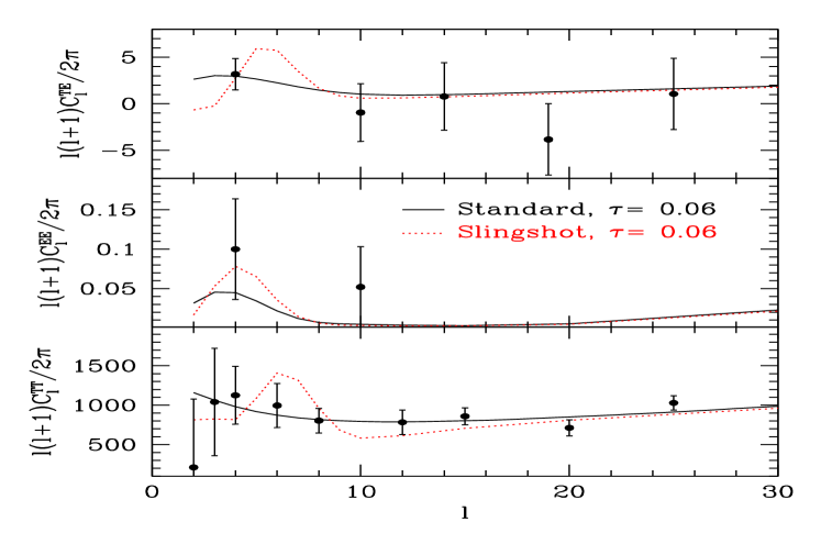
Figure 4: We consider a relatively low value of the optical depth to reionization, $\tau=0.06$, and study the effect of varying the normalization parameter $B$ in order to look for possible degeneracies between $\tau$ and $B$. The solid black line is the standard inflationary power spectrum whereas the dotted red line is the Slingshot prediction for a suitably large value of $B$. Even if we can improve the fit of polarization data with respect to the standard case, we produce a bump in low-$\ell$ temperature spectrum which does not allow to fit the data well ($\Delta\chi^{2}=1219$) .

The CMB temperature and polarization angular power spectra are obtained from the primordial power spectrum of scalar perturbations $P(k)$ through the well-known formula (see e.g. Seljak ):

$$C^{XX}_{\ell}=(4\pi)^{2}\int_{k_{min}}^{k_{max}}dkk^{2}P(k)(\Delta^{X}_{\ell}(k))^{2}\;,$$ (8)

where $\Delta^{X}_{\ell}(k)$ are the radiation transfer functions and $X=T,E$ defines temperature and polarization respectively. The temperature and polarization transfer functions can be extracted from a Boltzmann code like e.g. CMBfast. The angular power spectrum predicted by the Slingshot scenario can then be calculated starting from the primordial power spectrum of formula (7) and numerically evaluating the Lambert W-functions. The Slingshot power spectrum expression contains two new free parameters: the cut-off scale $k_{cut-off}$ and the amplitude $B$ of the large scale part $P_{blue}(k)$. We will now study the effects of varying these parameters on the final $C_{\ell}$s.

The first alternative we consider is to choose $k_{cut-off}$ such that $k_{cut-off}\ll k_{min}$ where $k_{min}$ is the smallest wavenumber appearing in the integral defined by eqn. (8). A cut-off below $k_{min}$ then clearly affects only scales that are unobservable. The choice of $B$ is then not relevant in this case and we can replace $P(k)$ in eqn. (8) with $P_{red}(k)$ defined in eqn. (2). We calculated the CMB power spectrum using this power spectrum and transfer functions obtained from the WMAP 3-years best-fit cosmological parameters. The resultant Slingshot $C_{\ell}$s in this case are represented by the dot-dashed green line in Figure 1. In the same Figure, the solid black line represents the standard WMAP best-fit power spectrum. The two spectra present a very good match, thus showing that, just by fitting the two parameters $A$ and $k_{0}$, the Slingshot model allows to well reproduce the standard CMB angular power spectrum from WMAP. More precisely, an explicit calculation of the likelihood for the Slingshot shows that the goodness-of-fit relative to the standard WMAP 3-years spectrum is $\Delta\chi^{2}_{eff}=3$, which, being non statistically significant wmap , makes the slingshot still a good fit of the data. As we were already stressing above, this result was not obvious due to the non-trivial running of the Slingshot primordial power spectrum.

Let us now consider a cut-off on scales that are relevant for the CMB, i.e. $k_{cut-off}\gtrsim k_{min}$ in eqn. 8.

In this case the wavenumber $k_{cut-off}$ will roughly define an angular cut-off $\ell_{cut-off}$ below which the angular power spectrum is basically obtained from a constant primordial power spectrum $P(k)=P_{\tiny blue}\equiv B/k_{0}^{3}$ (see eqn. (7)). At this point we found it useful for our analysis to determine a value of the normalization parameter $B$ which makes the amplitudes of $P_{\tiny red}(k)$ and $P_{\tiny blue}(k)$ to roughly coincide at the pivot scale (that we chose to be $k\sim 10^{-3}$ in our analysis). In order to match WMAP data for $\ell>\ell_{cut-off}$ we need $|k^{3}P_{\tiny red}(k)|\sim 10^{-10}$. Thus matching the two amplitudes yields:

$$k_{p}^{3}\frac{B}{k_{0}^{3}}=k_{p}^{3}P_{\tiny red}(k_{p})\sim 10^{-10}\;.$$ (9)

With our values of $k_{0}\sim 10^{-6}$ and $k_{p}\sim 10^{-3}$, we get $B\equiv\bar{B}\sim 10^{-19}$. We can now distinguish between two cases: $B\ll\bar{B}$ and $B\gtrsim\bar{B}$.

Let us firstly take $B\ll\bar{B}$ and consider several different $k_{cut-off}$. In this case the amplitude of $P_{\tiny blue}$ is much smaller than the amplitude of $P_{\tiny red}$. We then expect to see a suppression of power on scales $\ell<\ell_{cut-off}$. This is shown in figures 1 and 2. The same pictures also suggest that a cut-off scale $k_{\mbox{\tiny cut-off}}\lesssim 2\times 10^{-4}$ is still a good-fit to the data: the goodness-of-fit relative to the WMAP best-fit spectrum is $\Delta\chi^{2}_{eff}\leq 3$ in this range (for a similar discussion applied to a different model see michele ).

Let’s now move to the case $B\gtrsim\bar{B}$. We can now choose $B$ large enough to eliminate the suppression of the larger angular scales that we have just described above. In Figure 3 we consider an angular cut-off scale $l_{cut-off}\sim 10$ and we show that a choice of the normalization $B\sim\bar{B}$ can significantly improve the goodness-of-fit relative to the case $B\ll\bar{B}$ with the same cut-off ($\Delta\chi^{2}_{eff}=-112$). In other words this suggests that a full likelihood analysis of the slingshot parameters (which is beyond the purpose of this work) would show some degeneracy between $k_{cut-off}$ and $B$. Nevertheless it is important to note that this does not allow to arbitrarily increase the cut-off scale. The slope of the angular power spectrum for $\ell<\ell_{cut-off}$ is indeed completely different in the two regimes and this becomes rapidly evident for large $\ell_{cut-off}$. We then conclude that also in this case any possible Slingshot-related signature is unfortunately confined to the first few CMB multipoles, characterized by a large cosmic variance. For this reason it seems impossible to use the CMB $TT$, $TE$, and $EE$ angular power spectra as a way to discriminate between Slingshot and standard inflationary cosmology. To this purpose further investigation in other directions might be interesting (e.g. non-Gaussian signatures, gravitational wave background).

Even if we give up the idea of finding specific observable signatures of the Slingshot model in the CMB temperature and polarization power spectra, we are still left with the interesting following question: if we assume the Slingshot as the scenario for the generation of primordial fluctuations, and we repeat the analysis of WMAP results in this framework, are we going to see any change in the final cosmological parameters? In the acoustic peaks region both the Slingshot and the inflationary power spectrum have the same slope, so we already know that the answer to the previous question is ‘no’ for most of the parameters. As the only differences can be at small $\ell$, it seems that the only parameter that can in principle be affected is the optical depth at reionization $\tau$. Let us elaborate on this. WMAP is known to predict a large optical depth to reionization $\tau\simeq 0.09$, or equivalently an early reionization at a redshift $z\sim 10$. The signature of this early reionization is mainly in the bump observed at low $\ell$ in the TE and EE angular power spectra: there wouldn’t be any primordial polarization signal on large angular scales in absence of early reionization. This conclusion still holds in the Slingshot scenario (it is only related to the physics of Compton scattering). However the low-$\ell$ part of the polarization spectrum is described in the Slingshot by three parameters, $B$, $k_{cut-off}$ and $\tau$. Possible degeneracies among these parameters could then eventually change the best-fit value of $\tau$.

In particular it might now happen that a value of $\tau$ significantly smaller than in the standard scenario could still allow a good fit of the low-$\ell$ polarization bump if we compensate for it by increasing the amplitude $B$. This also works in the opposite direction: we can increase $\tau$ and reduce $B$ accordingly. This mechanism is clearly very efficient if we limit ourselves to considering polarization data only. The situation however drastically changes when we account for temperature data. A large $\tau$ produces a low-$\ell$ bump in the TE and EE but it does not affect the TT power spectrum. A large $B$ instead produces a large enhancement of the low-$\ell$ TT power spectrum as well. This effect is not compatible with the data if we have to compensate for a very small (large) $\tau$ with a very large (small) $B$. In other words temperature data contribute to largely breaking the degeneracy between $\tau$ and $B$ that arises from polarization data alone. An example of this is in Figure 4 where we try to fit data with an optical depth $\tau=0.06$ and all the other WMAP parameters unchanged.

5 Conclusions

In this paper we have studied some phenomenological implications of the cosmological Slingshot scenario introduced in sling ; sling2 . In the first part of the paper we have derived an expression of the primordial power spectrum of cosmological perturbations arising from the Slingshot (formula 7). This expression generalizes previous results by sling ; sling2 in that it contains a blue contribution to the spectrum which had not been considered before. In the second part of the paper we have numerically computed the CMB temperature and polarization power spectra arising from the Slingshot primordial spectrum. Firstly we showed that a suitable choice of the Slingshot parameters allows to match Slingshot predictions with the WMAP 3-years best-fit power spectrum. More precisely we showed through a relative goodness-of-fit approach that the slingshot predictions are not, in a statistical sense, worse than the best WMAP fit of a power law primordial spectrum. This conclusion has been drown by fitting the slingshot power spectrum spectral index to be 0.95 (best WMAP fit) at some pivot scale and by keeping all the standard cosmological parameter unchanged. To gain a more precise insight it would be however very important to perform a Montecarlo analysis were all parameter, in particular the spectral index, can change. This might in principle find a better fit to the data. However, as the aim of the present paper was only to show that, with the same WMAP parameters, the slingshot power spectrum is a good fit of the data, the above mentioned complete statistical analysis is left for future work. In the last part of the paper we finally looked for possible specific signatures of the Slingshot in CMB data that could allow to distinguish it from the standard scenario. Unfortunately all the distinctive Slingshot features turn out to be confined to the low-$\ell$ part of the spectrum, where large cosmic variance dominated error bars prevent from any significant discrimination between the two scenarios.

References

- (1) Kolb EW and Turner MS 1990 The Early Universe Frontiers in Physics no. 69 (Addison-Wesley).
- (2) D. N. Spergel et al., “Wilkinson Microwave Anisotropy Probe (WMAP) three year results: arXiv:astro-ph/0603449.
- (3) M. Gasperini and G. Veneziano, Phys. Rept. 373 (2003) 1 [arXiv:hep-th/0207130].
- (4) P. J. Steinhardt and N. Turok, Science 296 (2002) 1436.
- (5) C. Germani, N. E. Grandi and A. Kehagias, arXiv:hep-th/0611246.
- (6) C. Germani, N. E. Grandi and A. Kehagias, arXiv:0706.0023 [hep-th].
- (7) I. R. Klebanov and A. A. Tseytlin, Nucl. Phys. B 578, 123 (2000) [arXiv:hep-th/0002159].
- (8) A. Kehagias and E. Kiritsis, JHEP 9911 (1999) 022 [arXiv:hep-th/9910174].
- (9) M. R. Douglas and S. Kachru, [arXiv:hep-th/0610102].
- (10) M. Liguori, S. Matarrese, M. Musso and A. Riotto, JCAP 0408 (2004) 011 [arXiv:astro-ph/0405544].
- (11) S. Hollands and R. M. Wald, Gen. Rel. Grav. 34, 2043 (2002) [arXiv:gr-qc/0205058]. S. Hollands and R. M. Wald, arXiv:hep-th/0210001.
- (12) L. Kofman, A. Linde and V. F. Mukhanov, JHEP 0210, 057 (2002) [arXiv:hep-th/0206088].
- (13) R. Brandenberger, H. Firouzjahi and O. Saremi, arXiv:0707.4181 [hep-th].
- (14) A. R. Liddle and D. H. Lyth, “Cosmological inflation and large-scale structure,” (Cambridge Univiverity Press, Cambridge, UK, 2000)
- (15) V. Faraoni and S. Nadeau, Phys. Rev. D 75 (2007) 023501 [arXiv:gr-qc/0612075].
- (16) R.M. Corless, G.H. Gonnet, D.E.G. Hare, D.J. Jaffrey and D. Knuth, Adv. Comp. Math. 5 (1996)329.
- (17) U. Seljak, M. Zaldarriaga, Astrophys.J. 469 (1996) 437-444 [arXiv:astro-ph/9603033].