Diffusive radiation in Langmuir turbulence produced by jet shocks

Abstract

Anisotropic distributions of charged particles including two-stream distributions give rise to generation of either stochastic electric fields (in the form of Langmuir waves, Buneman instability) or random quasi-static magnetic fields (Weibel and filamentation instabilities) or both. These two-stream instabilities are known to play a key role in collisionless shock formation, shock-shock interactions, and shock-induced electromagnetic emission. This paper applies the general non-perturbative stochastic theory of radiation to study electromagnetic emission produced by relativistic particles, which random walk in the stochastic electric fields of the Langmuir waves. This analysis takes into account the cumulative effect of uncorrelated Langmuir waves on the radiating particle trajectory giving rise to angular diffusion of the particle, which eventually modifies the corresponding radiation spectra. We demonstrate that the radiative process considered is probably relevant for emission produced in various kinds of astrophysical jets, in particular, prompt gamma-ray burst spectra, including X-ray excesses and prompt optical flashes.

1 Introduction

Formation of collisionless astrophysical shocks, their interaction with ambient medium and each other are tightly coupled with two-stream instabilities giving rise to generation of either electric or magnetic fields or both in the shock vicinity. In the simplest kinetic version of the two-stream instability a tenuous electron beam excites Langmuir waves resonantly (i.e., at $k=\omega_{\rm pe}/v_{b}$, where $k$ is the Langmuir wave vector, $\omega_{\rm pe}$ is the background plasma frequency, $v_{b}$ is the velocity of the electron beam) on the linear stage of the instability. However, even though these small-scale Langmuir waves can initially be generated by the wave-particle resonance, non-linear wave-wave interactions will then transform the wave energy to larger scales (Kaplan & Tsytovich, 1973). Modern numerical models support that very small-scale random fields are generated initially at the shock front and then they evolve to larger and larger scales (Jaroschek et al., 2004, 2005; Nishikawa et al., 2003, 2005). Curiously, most of the work focuses on generation of stochastic magnetic fields due to Weibel or filamentation instabilities, although highly efficient charged particle acceleration occurring at the shock fronts necessarily requires generation of stochastic electric field as well (Bykov & Uvarov, 1993, 1999). Indeed, numerical simulations of relativistic shocks (e.g., Nishikawa et al., 2005) reveal very strong fluctuations of the electric charge $\rho$, which are tightly linked (${\bf kE}=4\pi\rho$) with the longitudinal electric fluctuations.

Quasilinear approach performed mainly analytically (Bret et al., 2005) in 3-dimensional case shows that oblique modes dominate both purely longitudinal and purely transverse modes. This is true also for the case when a magnetic field parallel the beam velocity direction is included (Bret et al., 2006) even though this magnetic field can completely suppress the purely transverse filamentation and Weibel modes. Both magnetic and electric fields are produced in the oblique modes and either electric or magnetic energy density can dominate depending on situation. Being excited these waves are subject of sophisticated evolution due to interaction with each other and with charged particles (Silva, 2006). These processes are deeply nonlinear and highly sensitive to the input parameters of the particular model.

Accordingly, there can be regimes when magnetic (electric) inhomogeneities are dominant during the entire evolution of the system and the effect of the electric (magnetic) inhomogeneities can be discarded. For example, Dieckmann (2005) considered an ultrarelativistic regime of the two-stream instability when a broad spectrum of Langmuir waves (including non-resonant, large-scale, ones $k\ll\omega_{\rm pe}/v_{b}$) is excited and persist for a long time in the plasma. However, different regimes when initially dominant magnetic turbulence then gives a way to the electric turbulence and vice versa are also possible (for a more instructive review, see Silva, 2006). It would, therefore, be highly desirable to have observational tests allowing to distinguish between these different regimes, which can only come from adequate interpretation of electromagnetic emission recorded from an object.

Surprisingly, the radiation arising as relativistic charged particles interact with stochastic electric fields of the Langmuir turbulence has not been studied yet in sufficient detail, even though a number of important and useful results have been obtained for the past 40 years. Initially, this radiative process was considered by Gailitis & Tsytovich (1964) (see also Kaplan & Tsytovich, 1973) for the case of small-scale Langmuir waves ($k\gg\omega_{\rm pe}/c$, $c$ is the speed of light) and then the theory was extended to the case of the spatially uniform ($k=0$) electric fluctuations with the plasma frequency (Tsytovich & Chikhachev, 1969). The issue of the characteristic frequency of this emission process was addressed by Melrose (1971), who call it after Colgate (1967) ”electrostatic bremsstrahlung” in contrast to ”magneto bremsstrahlung”, while Schlickeiser (2003) considered the total power of this process in a monochromatic approximation.

Getmantsev & Tokarev (1972) and Chiuderi & Veltri (1974) demonstrated that an ensemble of relativistic electrons interacting with the Langmuir turbulence would produce the emission with the same spectral index as for standard synchrotron radiation. The degree of polarization (for the case of highly anisotropic, one-dimensional Langmuir turbulence) was found to be as large as for synchrotron radiation in a uniform magnetic field (Tsytovich & Chikhachev, 1969; Kaplan & Tsytovich, 1973; Windsor & Kellogg, 1974). Therefore, one might conclude that these two emission processes are undistinguishable observationally (e.g., Windsor & Kellogg, 1974). We believe, this conclusion is too straightforward. Indeed, for a narrow energy distribution of emitting electrons or for a broad (power-law) distribution with sufficiently sharp low- and/or high- energy cut-off, the specral shapes of the emissions can be remarkably different, enabling us to distinguish between various radiative processes.

However, full description of possible spectral regimes of this radiative process has not been presented yet, although the general theoretical foundation for this is readily available (Toptygin & Fleishman, 1987; Toptygin et al., 1987; Fleishman, 2005, 2006b). In particular, Toptygin & Fleishman (1987) clearly demonstrated that the emission in the presence of random electric fields berries a lot of general similarities to the emission in the random magnetic fields (so called diffusive synchrotron radiation, DSR, Fleishman, 2005, 2006b), although the exact expression for the electron scattering rate should be adjusted accordingly to properly take into account the polarization and dispersion of the Langmuir waves. The physics lying behind these similarities relates to the diffusive random walk of the emitting particle as it is being randomly scattered by either electric or magnetic irregularities. To emphasize that this diffusive motion is a key property to describe the emission correctly, we will refer to this emission process as ”Diffusive Radiation in Langmuir turbulence” (or DRL) to be distinguished from its cousin DSR. So far, there is a number of terms suggested for this emission process, e.g., inverse Compton scattering of the plasma waves, inverse plasmon scattering, and electrostatic bremsstrahlung, although none of them is commonly accepted, since none of the titles is indicative enough for the radiative process considered. It is worth noting that the term ”electrostatic bremsstrahlung” is not well suited for the emission in the Langmuir waves because a more usual ”bremsstrahlung” is even more ”electrostatic”, than the DRL process discussed here.

2 Perturbation theory of DRL

Perturbative treatment of electromagnetic emission by a charged particle assumes that the particle moves rectilinearly with constant velocity but takes into account non-zero acceleration of the particle in the external field. This perturbative treatment is widely used because of its simplicity. Typically, one calculates first the particle acceleration ${\bf w}(t)$ due to a given field along the rectilinear trajectory and then uses this expression obtained for ${\bf w}(t)$ to find the radiation spectrum. In the case of a random external field, however, when ${\bf w}(t)$ is also a random function of time $t$ it is more convenient to express the radiation intensity via spatial and temporal spectrum of the external electric and/or magnetic field.

Within theoretical formulation proposed by Fleishman (2006b) the spectral and angular distribution of the emission produced by a single particle with the Lorenz-factor $\gamma$ in a plasma with random field has the form:

$$W_{{\bf n},\omega}^{\bot}=\frac{(2\pi)^{3}Q^{2}}{M^{2}c^{3}\gamma^{2}V}\left(\frac{\omega}{\omega^{\prime}}\right)^{2}\left[1-\frac{\omega}{\omega^{\prime}\gamma_{*}^{2}}+\frac{\omega^{2}}{2\omega^{\prime 2}\gamma_{*}^{4}}\right]\int dq_{0}d{\bf q}\delta(\omega^{\prime}-q_{0}+{\bf qv})\mid{\bf F}_{q_{0},{\bf q}\bot}\mid^{2}.$$ (1)

where $\gamma_{*}=\left(\gamma^{-2}+\frac{\omega_{\rm pe}^{2}}{\omega^{2}}\right)^{-1/2}$, $Q$, $M$, and $\gamma\gg 1$ are the charge, mass, and Lorenz-factor of the emitting particle, $V$ is the volume of the emission source, ${\bf F}_{q_{0},{\bf q}\bot}$ is the Fourier component at the frequency $q_{0}$ and the wave vector ${\bf q}$ of the Lorenz force transverse to the emitting particle velocity,

$$\omega^{\prime}=\frac{\omega}{2}\left(\gamma^{-2}+\theta^{2}+\frac{\omega_{\rm pe}^{2}}{\omega^{2}}\right),$$ (2)

$\theta\ll 1$ is the angle between the wave vector of emitted wave ${\bf k}=k{\bf n}$ and the particle velocity vector ${\bf v}$, $\omega$ is the emitted frequency. Contribution $W_{{\bf n},\omega}^{\bot}$ (marked with the superscript $\bot$) is provided by a component of the particle acceleration transverse to the particle velocity. In case of the electric (in contrast to magnetic) field, there is also a component of the acceleration along the particle velocity. The corresponding contribution has the form

$$W_{{\bf n},\omega}^{\|}=\frac{2(2\pi)^{3}Q^{4}}{M^{2}c^{3}\gamma^{6}V}\left(\frac{\omega}{\omega^{\prime}}\right)^{3}\left[1-\frac{\omega}{2\omega^{\prime}\gamma_{*}^{2}}\right]\int dq_{0}d{\bf q}\delta(\omega^{\prime}-q_{0}+{\bf qv})\mid{\bf E}_{q_{0},{\bf q}\|}\mid^{2},$$ (3)

which is typically small by a factor $\gamma^{-2}$ compared with the transverse contribution. Nevertheless, there exist special cases (e.g., a particle moving along one-dimensional turbulent electric field) when the transverse contribution is zero or very small and the parallel contribution comes to play. For example, this is the case when a charge particle moves along the electric field of one-dimensional Langmuir turbulence (Fleishman & Toptygin, 2007).

However, below we will consider only the transverse contribution, which is indeed the dominant one in most of the cases. Accordingly, the spectral distribution of the radiated energy is given by integration of (1) over the full solid angle $d\Omega=\sin\theta d\theta d\varphi\approx 2\pi d(\omega^{\prime}/\omega)$:

$$W_{\omega}^{\bot}=\frac{(2\pi)^{4}Q^{2}}{M^{2}c^{3}\gamma^{2}V}\int_{1/2\gamma_{*}^{2}}^{\infty}d\left(\frac{\omega^{\prime}}{\omega}\right)\left(\frac{\omega}{\omega^{\prime}}\right)^{2}\left[1-\frac{\omega}{\omega^{\prime}\gamma_{*}^{2}}+\frac{\omega^{2}}{2\omega^{\prime 2}\gamma_{*}^{4}}\right]\int dq_{0}d{\bf q}\delta(\omega^{\prime}-q_{0}+{\bf qv})\mid{\bf F}_{q_{0},{\bf q}\bot}\mid^{2}$$ (4)

similar to the DSR case (Fleishman, 2006b), but with the Lorenz force ${\bf F}=Q{\bf E}$ specified by electric ${\bf E}$ in place of magnetic field.

2.1 One-wave approximation in the DRL theory

Let’s consider first the simplest case when there is only one long Langmuir wave with $k_{0}c\ll\omega_{\rm pe}$, where ${\bf k}_{0}$ is the wave-vector and $\omega_{\rm pe}$ is the frequency of the Langmuir wave, which was described long ago by Tsytovich & Chikhachev (1969). Here, the spatial and temporal spectrum of the electric field in this Langmuir wave takes a simple form

$$\mid{\bf E}_{\bot}(q_{0},{\bf q})\mid^{2}=A_{E}\frac{TV}{(2\pi)^{4}}\delta({\bf q}-{\bf k}_{0})(\delta(q_{0}-\omega_{\rm pe})+\delta(q_{0}+\omega_{\rm pe})),$$ (5)

where $A_{E}$ is specified by the energy density of the electric field in the wave. For example, for spatially uniform electric oscillations

$${\bf E}={\bf E}_{0}\cos\omega_{\rm pe}t,$$ (6)

we have $A_{E}=\mid{\bf E}_{0\bot}\mid^{2}/4$ .

Calculation of the radiation intensity is extremely easy in case of field spectrum (5). Indeed, substituting (5) into (1) and taking the integrals over frequency $q_{0}$ and wave-vector ${\bf q}$ using the $\delta$-functions, we obtain the emission intensity (i.e., the energy emitted per unit time per unit frequency interval per unit solid angle) by dividing (1) over $T$:

$$I_{{\bf n},\omega}^{\bot}=\frac{A_{E}Q^{4}}{2\pi M^{2}c^{3}\gamma^{2}}\left(\frac{\omega}{\omega^{\prime}}\right)^{2}\left[1-\frac{\omega}{\omega^{\prime}}\left(\gamma^{-2}+\frac{\omega_{\rm pe}^{2}}{\omega^{2}}\right)+\frac{\omega^{2}}{2\omega^{\prime 2}}\left(\gamma^{-2}+\frac{\omega_{\rm pe}^{2}}{\omega^{2}}\right)^{2}\right]\delta(\omega^{\prime}-\omega_{\rm pe}+{\bf k}_{0}{\bf v}).$$ (7)

Let’s discuss this emission intensity in more detail. Recall (2) that $\omega^{\prime}$ is a function of the emission angle $\theta$. On the other hand, because of the $\delta$-function in (7), $\omega^{\prime}$ is a fixed number for a given set of values $\omega_{\rm pe}$, ${\bf k}_{0}$, and ${\bf v}$:

$$\omega^{\prime}=\omega_{\rm pe}-{\bf k}_{0}{\bf v}.$$ (8)

Therefore, there is strict correlation between the emission frequency and direction, thus, only one distinct frequency can be emitted along a given direction.

Interestingly, emission intensity (7) depends only weakly on the actual ${\bf k}_{0}$ value as long as the condition $k_{0}c\ll\omega_{\rm pe}$ holds. In particular, for a long Langmuir wave the radiation intensity is almost the same as for the spatially uniform temporal oscillations of the electric field with the plasma frequency. The radiation intensity into full solid angle (which is the differential spectral power, i.e., the energy emitted per unit time per unit frequency range) is given by simple integration of (7) over $d(\omega^{\prime}/\omega)$ with the use of the $\delta$-function. It does depend on ${\bf k}_{0}$ only weakly and for ${\bf k}_{0}=0$ has the form

$$I_{\omega}^{\bot}=\frac{Q^{4}{\bf E}^{2}_{0\bot}}{4M^{2}c^{3}\gamma^{2}}\frac{\omega}{\omega_{\rm pe}^{2}}\left[1-\frac{\omega}{\omega_{\rm pe}}\left(\gamma^{-2}+\frac{\omega_{\rm pe}^{2}}{\omega^{2}}\right)+\frac{\omega^{2}}{2\omega_{\rm pe}^{2}}\left(\gamma^{-2}+\frac{\omega_{\rm pe}^{2}}{\omega^{2}}\right)^{2}\right],\qquad\omega<2\omega_{\rm pe}\gamma^{2}.$$ (9)

in full agreement with the result of Tsytovich & Chikhachev (1969).

The dispersion of the plasma (terms $\omega_{\rm pe}^{2}/\omega^{2}$) has almost no effect on the radiation intensity. The spectrum has unique asymptote $I_{\omega}\propto\omega^{1}$ at low frequencies, $\omega\ll\omega_{\rm pe}\gamma^{2}$ with a peak at $\omega_{max}=2\omega_{\rm pe}\gamma^{2}$. The emission intensity vanishes at higher frequencies.

Given that the radiation intensity for the case of single long Langmuir wave has only a weak dependence on the actual wavelength, it is tempting to extrapolate the presented results (in particular, spectrum (9) to the case when an ensemble of many long Langmuir waves exists in the source volume. Below we will see, however, that it is fundamentally incorrect, because the presence of the broad spatial spectrum of electric fluctuations makes a great difference compared with the one-wave case; general trends here are similar to those for the DSR in random magnetic fields (Fleishman, 2006b).

2.2 Perturbation theory for broad spatial spectrum

Following the derivation given by Fleishman (2006b), it is easy to find

$$\mid{\bf E}_{q_{0},{\bf q}\bot}\mid^{2}=\frac{TV}{(2\pi)^{4}}\left(\delta_{\alpha\beta}-\frac{v_{\alpha}v_{\beta}}{v^{2}}\right)K_{\alpha\beta}(q_{0},{\bf q})$$ (10)

where $K_{\alpha\beta}(q_{0},{\bf q})=C_{\alpha\beta}K(q_{0},{\bf q})$; $C_{\alpha\beta}=q_{\alpha}q_{\beta}/q^{2}$ for the Langmuir turbulence since the electric field vector is directed along the wave vector in the Langmuir waves, while $K(q_{0},{\bf q})$ is the temporal and spatial spectrum of the Langmuir turbulence. Substituting (10) into general expression (1) and dividing the result by $T$ we obtain spectral and angular intensity of DRL per unit time, which is convenient to write down in the form:

$$I_{{\bf n},\omega}=\frac{Q^{2}}{2\pi^{2}c}\left(\frac{\omega}{\omega^{\prime}}\right)^{2}\left[1-\frac{\omega}{\omega^{\prime}\gamma_{*}^{2}}+\frac{\omega^{2}}{2\omega^{\prime 2}\gamma_{*}^{4}}\right]q_{L}(\omega,\theta),$$ (11)

where $q_{L}(\omega,\theta)\equiv q_{L}(\omega^{\prime})$ is the effective scattering rate of the relativistic particle by the Langmuir turbulence, which plays a key role within the full non-perturbative treatment of the DRL:

$$q_{L}(\omega,\theta)=\frac{\pi Q^{2}}{M^{2}c^{2}\gamma^{2}}\int dq_{0}d{\bf q}\left(\delta_{\alpha\beta}-\frac{v_{\alpha}v_{\beta}}{v^{2}}\right)K_{\alpha\beta}(q_{0},{\bf q})\delta(\omega^{\prime}-q_{0}+{\bf q}{\bf v}).$$ (12)

To perform further calculations we have to specify the form of $K_{\alpha\beta}(q_{0},{\bf q})$. Initially, the streaming instability can give rise to highly anisotropic turbulent spectrum with a limiting case of purely one-dimensional turbulence, although randomization of the wave vectors will later result in more isotropic turbulence patterns. DRL generated in the presence of one-dimensional Langmuir turbulence is specifically discussed by Fleishman & Toptygin (2007). By contrast, here we assume that the Langmuir wave vectors are isotropically distributed and the spectrum $K(q_{0},{\bf q})$ can be approximated by a power-law above certain critical value $k_{0}$:

$$K(q_{0},{\bf q})=\frac{a_{\nu}k_{0}^{\nu-1}\left<E_{L}^{2}\right>q^{2}}{(k_{0}^{2}+q^{2})^{\nu/2+2}}\delta(q_{0}-\omega_{\rm pe}).$$ (13)

Here, the presence of the $\delta$-function is related to the assumption that the electric turbulence is composed of Langmuir waves all of which oscillate in time with the same frequency $\omega_{\rm pe}$; the normalization constant $a_{\nu}$ is set up by the condition $\int K(q_{0},{\bf q})dq_{0}d{\bf q}=\left<E_{L}^{2}\right>$, where $\left<E_{L}^{2}\right>$ is the mean square of the electric field in the Langmuir turbulence.

Now, substituting (13) into (12), taking the integrals over $dq_{0}$ and $d\cos\theta_{q}$ with the use of two available $\delta$-functions in (12), and then integrating over $dq$, we find

$$q_{L}(\omega,\theta)=\frac{4\pi^{2}a_{\nu}k_{0}^{\nu-1}\omega_{\rm st}^{2}}{\nu(\nu+2)c\gamma^{2}}\left\{\left(\frac{\omega^{\prime}-\omega_{\rm pe}}{c}\right)^{2}+k_{0}^{2}\right\}^{-\nu/2},$$ (14)

where $\omega_{st}=Q\left<E_{L}^{2}\right>^{1/2}/Mc$. Substitution of (14) into (11) yields:

$$I_{{\bf n},\omega}^{\bot}=\frac{2a_{\nu}k_{0}^{\nu-1}\omega_{\rm st}^{2}Q^{2}}{\nu(\nu+2)c^{2}\gamma^{2}}\left(\frac{\omega}{\omega^{\prime}}\right)^{2}\left[1-\frac{\omega}{\omega^{\prime}}\left(\gamma^{-2}+\frac{\omega_{\rm pe}^{2}}{\omega^{2}}\right)+\frac{\omega^{2}}{2\omega^{\prime 2}}\left(\gamma^{-2}+\frac{\omega_{\rm pe}^{2}}{\omega^{2}}\right)^{2}\right]\left\{\left(\frac{\omega^{\prime}-\omega_{\rm pe}}{c}\right)^{2}+k_{0}^{2}\right\}^{-\nu/2}.$$ (15)

Apparently, spectrum (15) looks rather differently from that in case of a single Langmuir wave (9). In particular, no $\delta$-function enters (15), thus, a continuum spectrum rather than distinct frequencies is emitted along any direction. Clearly, there remains a distinct contribution to the emission intensity when $\omega^{\prime}\approx\omega_{\rm pe}$. However, the range of the parameter space where this resonant condition holds is relatively narrow, so the ”non-resonant” contribution from the remaining part of the parameter space where $\omega^{\prime}\neq\omega_{\rm pe}$ can easily dominate the resonant contribution. To see this explicitly, consider the radiation intensity into the full solid angle by integration of (15) over $d\Omega$ that yields

$$I_{\omega}^{\bot}=2\pi\int_{1/2\gamma_{*}^{2}}^{\infty}I_{{\bf n},\omega}^{\bot}d\left(\frac{\omega^{\prime}}{\omega}\right)=\frac{8Q^{2}\gamma_{*}^{2}}{3\pi c}q_{L}(\omega),$$ (16)

where

$$q_{L}(\omega)=\frac{3\pi^{2}a_{\nu}k_{0}^{\nu-1}\omega_{\rm st}^{2}}{2\nu(\nu+2)c^{3}\gamma^{2}\gamma_{*}^{2}}\int_{1/2\gamma_{*}^{2}}^{\infty}d\left(\frac{\omega^{\prime}}{\omega}\right)\left(\frac{\omega}{\omega^{\prime}}\right)^{2}\left[1-\frac{\omega}{\omega^{\prime}}\left(\gamma^{-2}+\frac{\omega_{\rm pe}^{2}}{\omega^{2}}\right)+\frac{\omega^{2}}{2\omega^{\prime 2}}\left(\gamma^{-2}+\frac{\omega_{\rm pe}^{2}}{\omega^{2}}\right)^{2}\right]$$$$\left\{\left(\frac{\omega^{\prime}-\omega_{\rm pe}}{c}\right)^{2}+k_{0}^{2}\right\}^{-\nu/2}.$$ (17)

Here we express the radiation spectrum via the effective scattering rate $q_{L}(\omega)=\overline{q_{L}(\omega,\theta)}$ averaged over the emission angle $\theta$, which defines the general non-perturbative expressions of the radiation intensity. Note that this averaging is performed with an appropriate weight described by the factor $\left(\frac{\omega}{\omega^{\prime}}\right)^{2}\left[1-\frac{\omega}{\omega^{\prime}\gamma_{*}^{2}}+\frac{\omega^{2}}{2\omega^{\prime 2}\gamma_{*}^{4}}\right]$, which enters Eqns (11) and (15). This factor is important since $\omega^{\prime}$ is a function of the emission angle $\theta$ according to equation (2). Combination of (16) and (17) yields finally:

$$I_{\omega}^{\bot}=\frac{4\pi a_{\nu}k_{0}^{\nu-1}\omega_{\rm st}^{2}Q^{2}}{\nu(\nu+2)c^{2}\gamma^{2}}\int_{1/2\gamma_{*}^{2}}^{\infty}d\left(\frac{\omega^{\prime}}{\omega}\right)\left(\frac{\omega}{\omega^{\prime}}\right)^{2}\left[1-\frac{\omega}{\omega^{\prime}}\left(\gamma^{-2}+\frac{\omega_{\rm pe}^{2}}{\omega^{2}}\right)+\frac{\omega^{2}}{2\omega^{\prime 2}}\left(\gamma^{-2}+\frac{\omega_{\rm pe}^{2}}{\omega^{2}}\right)^{2}\right]$$$$\left\{\left(\frac{\omega^{\prime}-\omega_{\rm pe}}{c}\right)^{2}+k_{0}^{2}\right\}^{-\nu/2}.$$ (18)

This integral cannot be taken analytically in a general case, but it is easy to plot corresponding spectra numerically. Figure 1 displays these spectra for a representative set of involved parameters. There are prominent differences in the DRL spectra in case of a broad spectrum of the Langmuir waves compared with the one-wave spectrum ($\propto\omega^{1}$), which is plotted in the figure for comparison. Even though we cannot perform full analytical treatment of the spectrum, we can estimate the spectral shape in various frequency ranges. At low frequencies $\omega\ll\omega_{\rm pe}\gamma^{2}$, we can discard $\omega^{\prime}$ in (18) everywhere in the braces except narrow region of parameters when $\omega^{\prime}\approx\omega_{\rm pe}$. This means that for $\omega\ll\omega_{\rm pe}\gamma^{2}$ the integral is composed of two contributions. The first of them, a non-resonant one, arises from integration over the region, where $\omega^{\prime}\ll\omega_{\rm pe}$. Here, the emission is beamed within the characteristic emission angle of $\vartheta\sim\gamma^{-1}$ along the particle velocity. The integral converges rapidly, and so it may be taken along the infinite region, which produces a flat radiation spectrum, $I_{\omega}\propto\omega^{0}$, or $I_{\omega}\propto\omega^{2}$ at lower frequencies, $\omega<\omega_{\rm pe}\gamma$. However, as far as $\omega^{\prime}$ approaches $\omega_{\rm pe}$, a resonant contribution comes into play. Now, in a narrow vicinity of $\omega_{\rm pe}$, we can adopt

$$\left\{\left(\frac{\omega^{\prime}-\omega_{\rm pe}}{c}\right)^{2}+k_{0}^{2}\right\}^{-\nu/2}\propto\delta(\omega^{\prime}-\omega_{\rm pe}),$$ (19)

which results in a single-wave-like contribution, $I_{\omega}\propto\omega^{1}$. The full spectrum at $\omega<\omega_{\rm pe}\gamma^{2}$, therefore, is just a sum of these two contributions.

At high frequencies, $\omega\gg\omega_{\rm pe}\gamma^{2}$, the term $\omega^{\prime}$ dominates in the braces, so other terms can be discarded. Thus, a power-law tail, $I_{\omega}\propto\omega^{-\nu}$, typical for DSR high-frequency asymptote, arises in this spectral range, where there was no emission et all in case of a single Langmuir wave, §2.1.

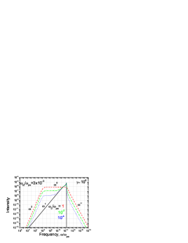
Figure 1: Perturbative DRL spectra produced by a particle with $\gamma=10^{6}$ in a plasma with relatively weak ($\omega_{\rm st}/\omega_{\rm pe}=3\cdot 10^{-3}$) long- and short- wave Langmuir turbulence for various $\omega_{0}/\omega_{\rm pe}$ ratios characterizing the turbulence: $\omega_{0}/\omega_{\rm pe}=1$, dashed/red curve; $\omega_{0}/\omega_{\rm pe}=10^{-2}$, dash-dotted/green curve; $\omega_{0}/\omega_{\rm pe}=10^{-4}$, dotted/blue curve. The spectrum of radiation in the presence of spatially uniform Langmuir oscillations (Tsytovich & Chikhachev, 1969) is shown by solid/black curve for comparison. The spectra contain a distinct spectral peak at $\omega\sim 2\omega_{\rm pe}\gamma^{2}$ for long-wave turbulence, which is absent for the short-wave turbulence.

Let’s compare the DRL spectra with the DSR spectra in case of stochastic magnetic fields (Fleishman, 2006b). If the Langmuir turbulence consists of relatively small-scale waves, $\omega_{0}\equiv k_{0}c\ \raise 3.0pt\hbox{$>$}\kern-8.5pt\raise-2.0pt\hbox{$\sim$}\ \omega_{\rm pe}$ (see dashed curve in Figure 1) then the shape of the spectrum is similar to the DSR spectrum. However, there is a remarkable difference in the case of the long-wave turbulence, $\omega_{0}\ll\omega_{\rm pe}$. Here, a distinct spectral peak at $\omega=2\omega_{\rm pe}\gamma^{2}$ is formed with the linear decrease of the spectrum with frequency, therefore, the immediate vicinity of the spectral peak can indeed be described within the single-wave approximation as suggested by Tsytovich & Chikhachev (1969). At lower frequencies, however, this falling part of the spectrum gives way to a flat spectrum, which is entirely missing within the one-wave approach. Position of the corresponding turning point depends on the $\omega_{0}/\omega_{\rm pe}$ ratio. It is worth emphasizing that the deviations of the DRL spectrum from the single-wave spectrum is prominent even for extremely long-wave turbulence, e.g., with $\omega_{0}/\omega_{\rm pe}=10^{-4}$ as in Figure 1. Therefore, the presence of a broad turbulence spectrum results in important qualitative change of the emission mechanism, which cannot generally be reduced to a simplified treatment relying on the single-wave approximation with some rms value of the Langmuir electric field.

3 Non-perturbative treatment of DRL

The perturbative treatment of the emission produced by a relativistic particle moving in the presence of random fields breaks down sooner or later as soon as intensity of the field and/or particle energy increase (e.g., Fleishman, 2006b). To find the applicability region of the perturbation theory applied above, we should estimate the characteristic deflection angle of the emitting electron on the emission coherence length $l_{c}=2c\gamma_{*}^{2}/\omega$, where the elementary emission pattern is formed. Similarly to Fleishman (2006b) consider a simple source model consisting of uncorrelated cells with the size $l_{0}=2\pi c/\omega_{0}$, each of which contains coherent Langmuir oscillations with the plasma frequency $\omega_{\rm pe}$. If $\omega_{0}>\omega_{\rm pe}$ then inside each cell the electron velocity will change by the angle $\theta_{0}\sim\omega_{\rm st}/(\omega_{0}\gamma)$, therefore, the consideration given in Fleishman (2006b) applies. However, if $\omega_{0}\ll\omega_{\rm pe}$, then the electric field vector will change the direction approximately $(\omega_{\rm pe}/\omega_{0})$ times during the time required for the particle to path through one cell, thus, the net deflection angle will be reduced by this factor $(\omega_{\rm pe}/\omega_{0})$ due to temporal oscillations of the electric field in the Langmuir waves, therefore $\theta_{0}\sim\omega_{\rm st}/(\omega_{\rm pe}\gamma)$. Then, after traversing $N=l_{c}/l_{0}$ cells, the mean square of the deflection angle is $\theta_{c}^{2}=\theta_{0}^{2}N\sim\omega_{\rm st}^{2}\omega_{0}/(\omega\omega_{\rm pe}^{2})$. The perturbation theory is only applicable if this diffusive deflection angle is smaller than the relativistic beaming angle, $\gamma^{-1}$, i.e., it is always valid at sufficiently high frequencies $\omega>\omega_{*}\equiv\omega_{\rm st}^{2}\omega_{0}\gamma^{2}/\omega_{\rm pe}^{2}$. Note, that the bounding frequency $\omega_{*}$ increases with $\omega_{0}$, while DSR displays the opposite trend. The perturbation theory will be applicable to the entire DRL spectrum if the condition $\theta_{c}^{2}<\gamma^{-2}$ holds for the frequency $\omega_{\rm pe}\gamma$ (Fleishman, 2006b), where the coherence length of the emission has a maximum. This happens for the particles whose Lorenz-factors obey the inequality

$$\gamma\ll\omega_{\rm pe}^{3}/(\omega_{\rm st}^{2}\omega_{0}).$$ (20)

We see, therefore, that generally, especially for relatively strong Langmuir turbulence, the perturbative treatment is insufficient to fully describe the radiation spectrum, thus, the non-perturbative version (Toptygin & Fleishman, 1987; Fleishman, 2005) of the theory should be explored. As demonstrated in Toptygin & Fleishman (1987) the same general expressions for the radiation intensity produced in the presence of stochastic electric fields are valid like in the random magnetic fields, although the electron scattering rate by Langmuir waves $q_{L}(\omega)=\overline{q_{L}(\omega,\theta)}$, which has already been introduced in the previous section, will differ from that in case of magnetic turbulence. As we will see below, all the differences between DRL spectrum in Langmuir turbulence and the DSR spectrum in magnetic turbulence are ultimately related to the difference in the expressions for the scattering rate $q_{L}(\omega)$ for these two cases.

Let’s consider first the regime when there is no regular magnetic field and, thus, the radiation spectrum is defined as (Fleishman & Bietenholz, 2007)

$$I_{\omega}=\frac{8Q^{2}q_{L}(\omega)}{3\pi c}\gamma^{2}\left(1+\frac{\omega_{\rm pe}^{2}\gamma^{2}}{\omega^{2}}\right)^{-1}\Phi(s),$$ (21)

where $\Phi(s)$ is the Migdal function (Migdal, 1954, 1956)

$$\Phi(s)=24s^{2}\int_{0}^{\infty}dt\exp(-2st)\sin(2st)\times\left[\coth t-\frac{1}{t}\right],\qquad\hbox{with}\ s=\frac{1}{8\gamma^{2}}\left(\frac{\omega}{q_{L}(\omega)}\right)^{1/2}\left(1+\frac{\omega_{\rm pe}^{2}\gamma^{2}}{\omega^{2}}\right)$$ (22)

having rather simple asymptotes for large or small $s$ values:

$$\Phi(s)\simeq 1,\hbox{if}\ s\gg 1,\qquad\Phi(s)\simeq 6s,\hbox{if}\ s\ll 1.$$ (23)

Figure 3 presents the DRL spectra for the case of relatively weak electric field, $\omega_{\rm st}\ll\omega_{\rm pe}$; the dash-dotted curves are the corresponding perturbative spectra. The non-perturbative effect (multiple scattering of the radiating electron by Langmuir waves) modifies the spectrum around the frequency $\omega_{\rm pe}\gamma$ giving rise to asymptote $I_{\omega}\propto\omega^{1/2}$ in this spectral region. Note that the frequency $\omega_{*}$, where the break from the $\propto\omega^{0}$ to $\propto\omega^{1/2}$ asymptote occurs, increases with $\omega_{0}$ increase, while the DSR in the static random magnetic fields (Fleishman, 2006b) displays the opposite trend.

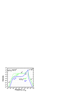
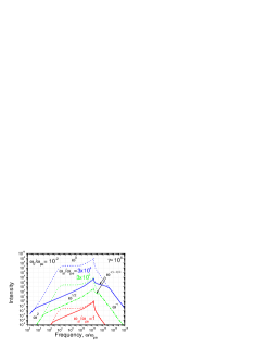
Figure 2: DRL spectra produced by highly relativistic particle with $\gamma=10^{10}$ moving in a plasma with long-wave Langmuir turbulence. Full non-perturbative spectra are shown by solid curves, while the corresponding perturbative spectra are by dashed and dash-dotted curves.

Figure 3: DRL in the presence of strong long-wave Langmuir turbulence. Dotted curves are calculated within the perturbation theory. Extremely strong suppression of the DRL spectra compared with the perturbative ones is evident.

However, as shown in Silva (2006) the electrostatic field in the Langmuir waves generated at the shock front can be rather strong, e.g., of the order of nonrelativistic wave breaking limit, $\omega_{\rm st}\approx\omega_{\rm pe}$. In this case, the non-perturbative treatment is important at the full frequency range below the spectral peak at $2\omega_{\rm pe}\gamma^{2}$, Figure 3. For completeness of the possible DRL regimes considered, Figure 3 presents also the DRL spectra for the (less realistic) case of a very strong random electric field, $\omega_{\rm st}\gg\omega_{\rm pe}$. Here, the non-perturbative spectrum deviates from the perturbative one even at the frequencies above $2\omega_{\rm pe}\gamma^{2}$, giving rise to a suppressed spectrum $I_{\omega}\propto\omega^{-(\nu-1)/2}$ (compared with the perturbative one $I_{\omega}\propto\omega^{-\nu}$). At the lower frequencies, a very broad non-perturbative power-law region of the spectrum, $I_{\omega}\propto\omega^{1/2}$, is formed.

4 DRL vs synchrotron radiation

If both Langmuir turbulence and regular magnetic field are present in the source, then both DRL and synchrotron emission are generated. One could assume that the DRL is only relevant in extreme conditions when the Langmuir turbulence energy density exceeds that of the regular magnetic field (e.g., Melrose, 1971). It is not the case, however, because these two emission mechanisms are efficient in differing frequency domains.

Consider joint effect of the Langmuir turbulence and a regular magnetic field on the radiation spectrum. In this case full equations (30) from (Fleishman, 2005) together with the exact expression for $q_{L}(\omega)$ given by Eq. (17) should be used. It is worth emphasizing that the condition $\omega_{\rm Be}\ll\omega_{\rm pe}$, where $\omega_{\rm Be}$ is cyclotron frequency in the regular magnetic field, is sufficient for full applicability of the available stochastic theory of radiation for the case under study. This condition means that the distortion of the electron trajectory due to the regular magnetic field is small during the period of electric oscillations, thus, it is not needed to be small at any spatial scale, so no further restriction on values of $\omega_{0}$, $\omega_{\rm st}$, and $\omega_{\rm pe}$ is necessary.

Figure 5 shows examples of the spectra for the cases of short-wave or long-wave Langmuir turbulence superimposed on a regular magnetic field. The full spectrum consists of the standard synchrotron contribution (region $I_{\omega}\propto\omega^{1/3}$ with exponential cut-offs at low- and high-frequency edges) and DRL contribution, which is the most prominent at the high frequencies $\omega\gg\omega_{\rm Be}\gamma^{2}$, although it is also present at sufficiently low frequencies, where the spectrum $I_{\omega}\propto\omega^{2}$ is formed.

Figure 5 allows direct comparison of the DRL spectrum with that of the standard synchrotron radiation. We point out that these two emission processes occupy distinct frequency ranges if $\omega_{\rm Be}\ll\omega_{\rm pe}$. In particular, the synchrotron spectrum displays exponential cut-off at the frequencies $\omega>\omega_{\rm Be}\gamma^{2}$, while the DRL displays here flat of even rising spectrum up to $\omega\sim\omega_{\rm pe}\gamma^{2}$. This means that DRL can dominate this spectral range even if the energy density in the Langmuir turbulence is lower than the magnetic field energy density. This holds also for a power-law energy spectrum with a high-energy cut-off at some $\gamma_{\rm max}$ for the spectral range $\omega>\omega_{\rm Be}\gamma_{\rm max}^{2}$.

Moreover, in sufficiently dense plasmas DRL can dominate the entire radiation spectrum even for the conditions when the Langmuir turbulence energy density is much smaller the the magnetic energy density. This happens for relatively low-energy (although ultrarelativistic) electrons, whose synchrotron emission is significantly suppressed by the Razin-effect (referred also to as density effect). Figure 5 displays such an example. Here the turbulent energy density is ten times lower than the magnetic energy density. Radiation spectrum produced by higher energy electrons ($\gamma>120$ for the parameters selected to plot the figure) consists of both DRL and synchrotron contribution, although the later becomes narrower and weaker as $\gamma$ decreases. Eventually, for $\gamma<120$, the synchrotron contribution disappears being strongly suppressed by the Razin effect in contrast to the DRL spectrum, which is less sensitive to the density effect.

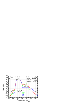
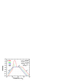
Figure 4: DRL spectra in the presence of uniform magnetic field with the energy density of the order of 10$\%$ of the Langmuir turbulence energy density. DRL dominates at frequencies above $\omega_{Be}\gamma^{2}$, where the perturbative treatment is applicable as long as $\omega_{\rm st}\ll\omega_{\rm pe}$.

Figure 5: DRL spectra in the presence of uniform magnetic field. The Langmuir turbulence energy density is of the order of 10$\%$ of the magnetic energy density. Synchrorton spectrum is strongly suppressed by the effect of density. DRL dominates the entire spectrum for sufficiently low-energy electrons with $\gamma<120$.

5 Discussion

Shock waves, in particular, jet shocks are believed to be the sites where various kinds of the two-stream instability can be operational. Depending on the conditions at the shock front and its vicinity either magnetic or electric fluctuations or both will be excited. Here, we specifically considered the case when random electric fields in a form of Langmuir wave turbulence dominate.

Modern computer simulations of shock wave interactions, especially in the relativistic case, suggest that the energy density of the excited Langmuir turbulence can be far in excess of the energy of the initial regular magnetic field. In particular, at the wave front the electric field can be as strong as the corresponding wave-breaking limit, i.e., $\omega_{\rm st}\sim\omega_{\rm pe}$. In this case the random walk of relativistic electrons in the stochastic electric field can give rise to powerful contribution in the nonthermal emission of an astrophysical object, entirely dominating full radiation spectrum or some broad part of it.

So far, the DRL (electrostatic bremsstrahlung) has been applied to a number of astrophysical objects. For example, Schlickeiser (2003) noted that electrostatic bremsstrahlung is an attractive alternative to standard synchrotron radiation to produce the observed nonthermal emission from jets in active galactic nuclei. In addition, Schröder et al. (2005) developed a simplified model of the galactic diffuse sub-MeV emission based on monochromatic approximation of both synchrotron radiation and the DRL, which gives rise to a remarkably good agreement between the model and the observations. We point out that the use of presented here DRL spectra will be helpful to further develop that model especially in the range of high-energy cut-off of the radiation spectra.

Although any detailed application of the considered emission process is beyond the scope of this paper, we mention that the DRL is also a promising mechanism for the gamma-ray bursts and extragalactic jets. In particular, some of the prompt gamma-ray bursts display rather hard low-energy spectra with the photon spectral index $\alpha$ up to 0. The DRL spectral asymptote $I_{\omega}\propto\omega^{1}$, which appears just below the spectral peak at $2\omega_{\rm pe}\gamma^{2}$, fits well to those spectra. Remarkably, the flat lower-frequency asymptote, $I_{\omega}\propto\omega^{0}$, can account for the phenomenon of the X-ray excess (Preece et al., 1996; Sakamoto et al., 2005) and prompt optical flashes accompanying some GRBs.

In addition, this mechanism (along with the DSR in random magnetic fields, Fleishman, 2006a) can be relevant to the UV-X-ray flattenings observed in some extragalactic jets. For example, although full spatially resolved radio to X-ray spectra of the jet in M87 agrees well with the DSR model (Fleishman, 2006a), for the jet in 3C 273 this agreement holds from the radio to UV range, while its X-ray emission seems to require an additional component (Jester et al., 2006). Alternatively, the entire UV-to-X-ray spectrum of 3C 273 might be produced by DRL, which can be much flatter than usual DSR (see, e.g., Figure 5) in the range $\omega_{\rm Be}\gamma^{2}\ll\omega\ll\omega_{\rm pe}\gamma^{2}$.

References

- Bret et al. (2006) Bret A., Dieckmann M. E., Deutsch C., 2006, Physics of Plasmas, 13, 2109
- Bret et al. (2005) Bret A., Firpo M.-C., Deutsch C., 2005, Physical Review Letters, 94, 115002
- Bykov & Uvarov (1993) Bykov A. M., Uvarov Y. A., 1993, JETP Letters, 57, 644
- Bykov & Uvarov (1999) Bykov A. M., Uvarov Y. A., 1999, JETP, 88, 465
- Chiuderi & Veltri (1974) Chiuderi C., Veltri P., 1974, A&A, 30, 265
- Colgate (1967) Colgate S. A., 1967, ApJ, 150, 163
- Dieckmann (2005) Dieckmann M. E., 2005, Physical Review Letters, 94, 155001
- Fleishman (2005) Fleishman G. D., 2005, ArXiv Astrophysics e-prints, astro-ph/0510317
- Fleishman (2006a) Fleishman G. D., 2006a, MNRAS, 365, L11
- Fleishman (2006b) Fleishman G. D., 2006b, ApJ, 638, 348
- Fleishman & Bietenholz (2007) Fleishman G. D., Bietenholz M. F., 2007, ArXiv Astrophysics e-prints
- Fleishman & Toptygin (2007) Fleishman G. D., Toptygin I. N., 2007, Phys. Rev. E, 75, 019706
- Gailitis & Tsytovich (1964) Gailitis A. K., Tsytovich V. N., 1964, Soviet Phys. – JETP, 19, 1165