Odd-Integer Quantum Hall Effect in Graphene: Interaction and Disorder Effects

Abstract

We study the competition between the long-range Coulomb interaction, disorder scattering, and lattice effects in the integer quantum Hall effect (IQHE) in graphene. By direct transport calculations, both $\nu=1$ and $\nu=3$ IQHE states are revealed in the lowest two Dirac Landau levels. However, the critical disorder strength above which the $\nu=3$ IQHE is destroyed is much smaller than that for the $\nu=1$ IQHE, which may explain the absence of a $\nu=3$ plateau in recent experiments. While the excitation spectrum in the IQHE phase is gapless within numerical finite-size analysis, we do find and determine a mobility gap, which characterizes the energy scale of the stability of the IQHE. Furthermore, we demonstrate that the $\nu=1$ IQHE state is a Dirac valley and sublattice polarized Ising pseudospin ferromagnet, while the $\nu=3$ state is an $xy$ plane polarized pseudospin ferromagnet.

A number of dramatic recent experiments G0 ; G2 ; Hall0 ; Hall1 have demonstrated the Dirac-like character of the low-energy electrons in graphene, a single monolayer film of carbon exfoliated from graphite. In a relatively weak magnetic field, where the Zeeman splitting is negligible, an unconventional quantization of the Hall conductivity is observed, $\sigma_{xy}=\nu\frac{e^{2}}{h}$ with $\nu=4(k+\frac{1}{2})$ and $k$ an integer Hall0 ; Hall1 . This can be ascribed to the Berry phase anomaly at the Dirac points Hall0 ; Hall1 ; T0 ; T1 ; T2 ; T3 and the four-fold spin and sublattice symmetry haldaneh (pseudospin) degeneracies of the Landau levels (LLs). Interestingly, additional odd-integer $\nu=\pm 1$ Hall plateaus together with even-integer $\nu=\pm 2,\pm 4...$ Hall plateaus were observed in a recent experiment ODDHall by using a strong magnetic field. A magnetic field which is sufficiently strong to lift the spin degeneracy of the LLs is expected to produce the quantization rule $\nu=2k$, as illustrated in Fig. 1, which explains only the even-integer Hall plateaus.

The even parity of $\nu$ is assured in the clean, non-interacting limit by the valley degeneracy of the two Dirac points, which in turn is protected by the point-group symmetry of ideal graphene. The odd-integer quantum Hall effect (IQHE) is considered by most authors to be caused by electron-electron interactions macodd ; fisherodd ; ODDHallT2 ; ODDHallT3 ; ODDHallT4 ; ODDHallT5 . These works obtain a pseudospin ferromagnetic (PFM) $\nu=1$ state macodd ; fisherodd ; ODDHallT2 ; ODDHallT3 ; ODDHallT4 ; ODDHallT5 associated with Haldane’s repulsive pseudopotential haldane , based on the low-energy continuum two-valley Dirac fermion description. In the continuum limit, the point-group and spin-rotation symmetries of the material are elevated to a full SU(4) symmetry, which reduces to an SU(2) symmetry when Zeeman splitting is introduced. Using the Stoner criterion macodd , Nomura and MacDonald have obtained a phase diagram, where the $\nu=1$ IQHE state has a much lower critical magnetic field than the $\nu=3$ state for a given sample mobility. However, direction of the SU(2) symmetry breaking (orientation of the PFM magnetization) is not determined from the continuum theory. It depends instead upon residual effects of the lattice, as addressed by Alicea and Fisher fisherodd , who obtained an easy-axis orientation corresponding to sublattice (charge density wave) order in the $\nu=1$ state. Moreover, the energy gap measured in transport is also sensitive to disorder at the lattice scale. This is especially important here, because the low-energy excitations of the $\nu=\pm 1$ IQHE states may be gapless ODDHallT2 , which may lead to a non-trivial energy scale characterizing the stability of the IQHE. When the higher odd-integer Hall plateaus with $|\nu|>1$ are observable is still controversial. To resolve these issues, an exact account of the competition between the long-range Coulomb interaction, disorder, and lattice effects is desirable, but so far lacking.

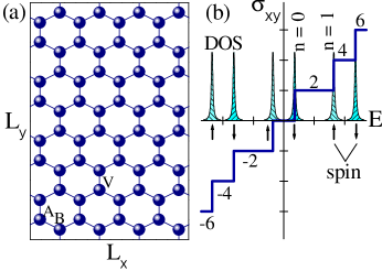
Figure 1: (color figure online) (a) A rectangular sample of graphene of size $L_{x}\times L_{y}$. (b) Illustration of the electron density of states of the LLs (filled area) and the even-integer quantized plateaus of the Hall conductivity $\sigma_{xy}$ (thick line) in the absence of electron interaction.

In this Letter, we carry out exact diagonalization calculations in a honeycomb lattice model, which captures all these effects naturally. Through direct transport calculations, we provide numerical evidence that the Coulomb interaction can induce the $\nu=\pm 1$ and $\pm 3$ Hall plateaus. It is shown that, when the disorder is relatively weak, a number of low-energy many-particle states carry a same constant Chern number, forming a mobility gap, which protects the IQHE. The critical disorder strength for the $\nu=1$ state, determined as the point where the mobility gap vanishes, is much greater than that for the $\nu=3$ state, suggesting that the $\nu=3$ IQHE may be observed experimentally if disorder scattering can be further suppressed. The $\nu=1$ state is clearly demonstrated to be a pseudospin ferromagnet with Ising anisotropy in the weak disorder regime. Moreover, our energy spectrum analysis indicates that a PFM order exists in the $\nu=3$ state with the easy axis polarized in the $xy$ plane, consistent with the theoretical suggestion fisherodd .

Our model Hamiltonian in a perpendicular field ${\bf B}$ is

$$H=H_{0}+\frac{1}{2}\sum\limits_{i,j}U({\bf R}_{i}-{\bf R}_{j})n_{i}n_{j}\ ,$$ (1)

where $H_{0}$ is the non-interacting Hamiltonian haldaneh ; donnah

$$H_{0}=-\sum_{\langle ij\rangle,\sigma}t_{ij}c_{i\sigma}^{\dagger}c_{j\sigma}+\sum_{i\sigma}\left(-g\sigma B+w_{i}\right)c_{i\sigma}^{\dagger}c_{i\sigma},$$ (2)

and the second term in Eq.(1) is the Coulomb interaction. Here, $n_{i}=\sum_{\sigma}c_{i\sigma}^{\dagger}c^{\vphantom{\dagger}}_{i\sigma}$ is the electron number operator on site $i$, $t_{ij}=te^{ia_{ij}}$ is the electron hopping amplitude between neighboring sites in the presence of a magnetic flux $\phi=\sum_{{\small{\mbox{\hexagon}}}}a_{ij}=\frac{2\pi}{M}$ per hexagon donnah with $M$ an integer, $g\sigma B$ is the Zeeman coupling energy with $\sigma=\pm 1$ for electron spin parallel and antiparallel to ${\bf B}$, and $w_{i}$ is a random on-site potential uniformly distributed between $[-W/2,W/2]$, accounting for nonmagnetic disorder. Denoting the nearest neighbor carbon-carbon distance by $a_{0}$, the magnetic length $\ell$ defined as usual is given by $\ell^{2}=\frac{3\sqrt{3}}{4\pi}Ma_{0}^{2}$.

We first diagonalize the noninteracting Hamiltonian $H_{0}$ on a rectangular sample (Fig. 1a), and obtain the complete set of single-particle wave functions of $H_{0}$. For the range of fields and disorder strengths considered here, the LL broadening from disorder scattering is always small compared to the LL spacing, and so the states associated to a given LL are clearly identifiable. We assume that the magnetic field is strong enough to cause complete splitting of the LLs for two spin directions. The total degeneracy of each LL near band center is denoted as $2N_{s}$ for each spin, i.e., $N_{s}(=\frac{L_{x}L_{y}}{2M})$ is the degeneracy for each Dirac component. We define $N_{e}$ as the electron number in the highest occupied LL – the $n^{\rm th}$ – such that the number of electrons counted from the band center is $2nN_{s}+N_{e}$, with $0\leq N_{e}<2N_{s}$. The filling number is $\nu=2n+N_{e}/N_{s}$. Because of full spin polarization, the relevant matrix elements of the Coulomb interaction are those with $i\neq j$, which are taken to be $U({\bf R}_{i}-{\bf R}_{j})=Va_{0}/|{\bf R}_{i}-{\bf R}_{j}|$. The Coulomb interaction is projected into the $n$-th LL, and the many-particle wavefunctions are solved exactly in the subspace of the LL.

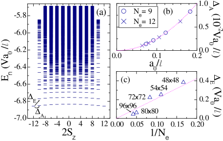
Figure 2: (color figure online) (a) The energy spectrum in the units $Va_{0}/\ell$ as a function of total pseudospin $2S_{z}$ calculated for a sample size of $96\times 96$ and $M=4\times 96$ at $\nu=1$ ($N_{e}=12$) in the clean limit ($W=0$). Here, the static Coulomb interaction energy has been included, and the irrelevant constant Zeeman energy shift has been omitted. (b) Anisotropic gap energy $\Delta_{\mbox{\tiny A}}$ as a function of $a_{0}/\ell$, where the sample sizes range from $36\times 36$ to $120\times 120$ for $N_{e}=12$ and $N_{e}=9$. The dotted line represents a parabolic fit to the data. (c) Excitation gap $\Delta_{\mbox{\tiny E}}$ as a function of $1/N_{e}$ with the dotted line as a linear fit. The values of $M$ are chosen so that $\nu=1$ or $N_{s}=N_{e}$.

.

For filling number $0<\nu<2$, the Fermi energy is located inside the lowest $n=0$ LL. Denoting by $A,B$ the two sublattices of sites, the $z$-component of the pseudospin $S_{z}$ is expressed as $2S_{z}=\sum_{i\in A}n_{i}-\sum_{i\in B}n_{i}$ (in $\hbar=1$ units), which is conserved as the central LL eigenstates can be chosen to have support only on one of the two sublattices (the correction from lattice model is smaller than $10^{-8}$ for system sizes that we consider). In Fig. 2a, we show the calculated many-particle low-energy spectrum at $\nu=1$ for $W=0$ as a function of $2S_{z}$, where $L_{x}=L_{y}=96$, and $M=4\times 96$. Periodic boundary conditions are imposed in the $x$ and $y$-directions.

In Fig. 2a, the lowest row of $N_{e}+1$ energies corresponds to PFM states for $N_{e}+1$ different eigenvalues of $2S_{z}$ between $-N_{e}$ and $N_{e}$. The two with $2S_{z}=N_{e}$ and $-N_{e}$ have the lowest-energy, with intermediate values $-N_{e}<2S_{z}<N_{e}$ exhibiting higher energies. Clearly, this result suggests the presence of pseudospin anisotropy, with the $z-$axis as the easy axis fisherodd . In more physical terms, the favored $2S_{z}=\pm N_{e}$ values represent charge ordered states with electrons occupying only one sublattice. We can define an anisotropic energy $\Delta_{\mbox{\tiny A}}$ equal to the energy difference between the lowest eigenenergies at $2S_{z}=-N_{e}$ and at $2S_{z}=-(N_{e}-2)$. $\Delta_{\mbox{\tiny A}}$ calculated for several different sample sizes is shown in Fig. 2b as a function of $a_{0}/\ell$. The data can be well fitted by a parabolic function $\Delta_{\mbox{\tiny A}}\propto(a_{0}/\ell)^{2}$, which vanishes in the continuum limit faster than the characteristic Coulomb energy $Va_{0}/\ell$. This is consistent with the interpretation of the pseudospin anisotropy as arising from corrections due to lattice effects, resulting in an additional $a_{0}/\ell$ suppression factor.

In Fig. 2a, we also see a small energy gap $\Delta_{\mbox{\tiny E}}$ between the PFM ground state and the lowest excited state in the second lowest row. We calculated $\Delta_{\mbox{\tiny E}}$ for different values of electron number $N_{e}$ from $N_{e}=6$ up to $24$, as plotted in Fig. 2c as a function of $1/N_{e}$, where the magnetic flux strength $1/M$ is chosen to be nearly constant at different $N_{e}$, such that $N_{e}$ changes proportionally with the sample size $L_{x}\times L_{y}$. The data can be roughly fitted by a linear relation $\Delta_{\mbox{\tiny E}}\propto 1/N_{e}$. We note that in the absence of anisotropy, such gapless $\Delta_{\mbox{\tiny E}}\sim 1/L^{2}\sim 1/N_{e}$ behavior would be expected for the first excited pseudospin-wave states with $|q|\sim 1/L$. Though the Ising anisotropy would be expected to introduce a gap, the observed behavior is probably consistent with the rather small anisotropy energy (note the scale in Fig. 2b).

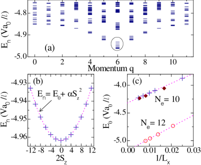
Figure 3: (color figure online) (a) The energy spectrum in the units $Va_{0}/\ell$ as a function of total momentum $q$ in Landau gauge calculated for a sample size $96\times 96$ and $M=4\times 96$ at $\nu=3$ ($N_{e}=N_{s}$) in the clean limit ($W=0$), (b) the $(N_{e}+1)$ lowest eigenenergies, as indicated by circle in (a), fitted by a parabolic function of total pseudospin $2S_{z}$, and (c) ground-state energy for $N_{e}=10$ and $N_{e}=12$ calculated for different sample sizes and $M$ with the dotted lines as a guide to the eye. In (c), for $N_{e}=10$, the cross and diamond symbols indicate Ising and $xy$ plane PFM states, respectively, and all systems with $N_{e}=12$ (circles) are in the $xy$ plane PFM state.

We have also carried out a spectral analysis for filling number $\nu=3$, where half states in the $n=1$ LL are filled. Though in the continuum limit, the absence of coupling between valleys means that the pseudospin is conserved in this LL, there is no obvious $S_{z}$ conservation on the lattice analogous to the $n=0$ case. We show in Fig. 3a the low-energy spectrum in each total momentum $q$ sector for pure system $W=0$ and system size $L_{x}=L_{y}=96$. Interestingly, the lowest $N_{e}+1$ energies are all in the $q=N_{e}/2$ (in units of $\frac{4\pi}{3L_{y}a_{0}}$) sector with no double occupancy of any of the pseudospin doublets. Thus they are low-energy spin excitations, which can be fitted into $\Delta E=(E_{n}-E_{0})=\alpha S_{z}^{2}$ (with $\alpha>0$) as shown in Fig. 3b. This suggests that the nondegenerate ground state has $S_{z}=0$, and is an $xy$ plane polarized PFM state, with strong valley mixing. We have further checked a number of system sizes between $24\times 24$ to $200\times 200$, and found that the $xy$ plane polarized state is always the ground state as long as both $L_{x}$ and $L_{y}$ are commensurate with 3 (that includes all the systems with $N_{e}=12$). Otherwise, an Ising PFM state is found to be favorable, as shown in Fig. 3c. This strong systematic finite-size effect can be understood from the graphene band structure, since valley mixing implies order at the wavevector connecting the two Dirac points, and hence period 3 modulations in both lattice directions note . Indeed $E_{0}$ shows an oscillation with an upturn at Ising points, indicating frustration of the modulations in the energetically preferred $xy$ PFM state. The $xy$ plane PFM state is expected to become the ground state for $\nu=3$ at the thermodynamic limit. The charge density is uniform in the $xy$ plane state with vanishing charge current on each lattice bond. Interestingly, in the Ising state, we observe lattice-scale charge currents circulating around one third of the hexagons in the pattern predicted by Alicea and Fisher fisherodd .

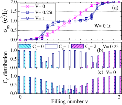
Figure 4: (color figure online) (a) Hall conductivity $\sigma_{xy}$ for disorder strength $W=0.1t$ and three different interaction strengths $V$, averaged over 40 disorder configurations. Here, $L_{x}=L_{y}=54$, $M=3\times 54$, and the error bars stand for the standard deviation due to disorder average. (b) and (c) are the probability distributions of the ground-state Chern number for $V=0.25t$ and $V=0$, respectively.

Given that any gap for the $\nu=1$ IQHE is small enough to be numerically unresolvable, it is important to directly demonstrate its robustness to disorder. We now calculate the Hall conductivity $\sigma_{xy}$, which can be expressed in terms of the ensemble average of the Chern number Chern0 ; mbgap $C_{0}$ of the ground state as $\sigma_{xy}=\frac{e^{2}}{h}\langle C_{0}\rangle$. In Fig. 4a, the calculated $\sigma_{xy}$, averaged over 40 random disorder configurations, is shown as a function of filling number for a weak disorder strength $W=0.1t$. In the absence of Coulomb interaction ($V=0$), $\sigma_{xy}$ increases continuously with $\nu$, without showing a quantized plateau around $\nu=1$. However, as the interaction is switched on, a quantized Hall plateau appears around $\nu=1$. In Fig. 4b, the Chern number distribution for $V=0.25t$ at filling numbers $\nu=0,\frac{1}{9},\cdots 2$ is shown. Near integer filling numbers $1$ and $2$, the Chern number takes constant values $C_{0}=1$ and $C_{0}=2$ for all disorder configurations without fluctuations, corresponding to the $\nu=1$ and $\nu=2$ IQHE plateaus in Fig. 4a, respectively. For $V=0$, as shown in Fig. 4c, various Chern numbers, $C_{0}$=$0$, $1$ and $2$, merge together in the middle region, resulting in a plateau-metal transition.

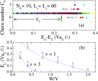
Figure 5: (color figure online) (a) Calculated Chern numbers of 60 low-energy eigenstates as a function of $E_{n}-E_{0}$ with $E_{n}$ the $n$-th eigenenergy at $\nu=1$, for $V=0.5t$, $W=0.8V$ and 10 random disorder configurations. (b) Critical energy $E_{\mbox{\tiny C}}$ for filling numbers $\nu=1$ (squares) and $\nu=3$ (triangles) as functions of normalized disorder strength $W/V$, where the error bars are the mean deviation of $E_{\mbox{\tiny C}}$ due to disorder sampling.

We now study the thermal stability of the odd IQHE by also considering the excited states. In Fig. 5a, we show the Chern numbers of 60 lowest eigenstates calculated at $\nu=1$ for $L_{x}=L_{y}=60$ and $N_{e}=10$ as a function of $E_{n}-E_{0}$. The Chern numbers for 10 random disorder configurations of strength $W=0.8V$ are represented by different symbols. We see that the Chern numbers of low-energy eigenstates with $E_{n}-E_{0}$ smaller than a critical energy $E_{c}$ always take a constant value $C_{n}=1$, indicating localization for these states and a mobility gap (which is directly related to the activation gap) of order $E_{\mbox{\tiny C}}$ mbgap . The calculated $E_{\mbox{\tiny C}}$ as a function of $W/V$ for $V=0.5t$ is shown in Fig. 5b (squares). For $W>W_{\mbox{\tiny C}}\simeq 2.0V$, $E_{\mbox{\tiny C}}$ diminishes to zero, where the $\nu=1$ IQHE is destroyed.

By similar calculations, we find that odd IQHE can also occur in higher LLs, in consistence with the $xy$ plane PFM order. The calculated phase diagram for $\nu=3$ IQHE in the $n=1$ LL is shown in Fig. 5b (triangles). The $\nu=3$ IQHE is less stable than the $\nu=1$ IQHE, with a critical disorder strength $W_{\mbox{\tiny C}}\simeq 0.6V$ about one third of that for $\nu=1$. This may explain the observation of the $\nu=1$ but not $\nu=3$ plateau in experiment ODDHall .

Acknowledgment: This work is supported by the National Basic Research Program of China 2007CB925104, the Robert A. Welch Foundation under the grant no. E-1146 (LS), the DOE grant DE-FG02-06ER46305, ACS-PRF 41752-AC10, the NSF grants DMR-0605696 (DNS) and DMR-0611562 (DNS, FDMH), the NSF under MRSEC grant/DMR-0213706 at the Princeton Center for Complex Materials (FDMH), the NSF grant/DMR-0457440 and the Packard Foundation (LB), and the support from KITP through NSF PHY05-51164.

References

- (1) K. S. Novoselov, , Science 306, 666 (2004).
- (2) Y. Zhang, J. P. Small, W. V. Pontius and P. Kim, Appl. Phys. Lett. 86, 073104 (2005); Y. Zhang, J. P. Small, M. E. S. Amori and P. Kim, Phys. Rev. Lett. 94, 176803 (2005).
- (3) K.S. Novoselov, , Nature 438, 197 (2005).
- (4) Y. Zhang, Y.-W. Tan, H. L. Stormer, and Philip Kim, Nature 438, 201 (2005).
- (5) V. P. Gusynin and S. G. Sharapov Phys. Rev. Lett. 95, 146801 (2005).
- (6) N. M. R. Peres, F. Guinea, A. H. Castro Neto, Phys. Rev. B 73, 125411 (2006).
- (7) E. McCann and V. I. Fal’ko, Phys. Rev. Lett. 96, 086805 (2006).
- (8) Y. Zheng and T. Ando, Phys. Rev. B 65, 245420 (2002).
- (9) F. D. M. Haldane, Phys. Rev. Lett. 61, 2015 (1988).
- (10) Y. Zhang, , Phys. Rev. Lett. 96, 136806 (2006).
- (11) K. Nomura and A. H. MacDonald, Phys. Rev. Lett. 96, 256602 (2006); M. M. Fogler and B. I. Shklovskii, Phys. Rev. B 52, 17366 (1995).
- (12) J. Alicea and M. P. A. Fisher, Phys. Rev. B 74, 075422 (2006); cond-mat/07063733 (2007).
- (13) K. Yang, S. Das Sarma, and A. H. MacDonald, Phys. Rev. B 74, 075423 (2006).
- (14) V. P. Gusynin, V. A. Miransky, S. G. Sharapov, and I. A. Shovkovy, Phys. Rev. B 74, 195429 (2006).
- (15) C. Toke and J. K. Jain, cond-mat/0701026 (2007).
- (16) M. O. Goerbig, R. Moessner, and B. Doucot, Phys. Rev. B 74, 161407 (2006).
- (17) F. D. M. Haldane, Phys. Rev. Lett. 51, 605 (1983).
- (18) D. N. Sheng, L. Sheng, and Z. Y. Weng, Phys. Rev. B 73, 233406 (2006).
- (19) For finite-size systems with periodic boundary conditions, the allowed wavevectors take a set of discrete values. The Dirac point wavevectors and are among the discrete set of wavevectors only when both and are multiples of .
- (20) D. J. Thouless et al., Phys. Rev. Lett. 49, 405 (1982); Q. Niu et al., Phys. Rev. B 31, 3372 (1985).
- (21) D. N. Sheng et al., Phys. Rev. Lett. 90, 256802 (2003); D. N. Sheng, L. Balents, and Z. Wang, ibid. 91, 116802 (2003); X. Wan et al, Phys. Rev. B 72, 075325 (2005).