Mixing and $CP$ violation in the $D^{0}$ and $B_{s}^{0}$ systems

Abstract

Recent developments for mixing and $CP$ violation in the $D^{0}$ – $\,\overline{\!D}{}{}^{0}$ and $B_{s}^{0}$ – $\,\overline{\!B}{}{}^{0}_{s}$ systems are reviewed, including (i) the recently emerging evidence for $D^{0}$ – $\,\overline{\!D}{}{}^{0}$ mixing and the interpretations of the measurements; (ii) the theoretical status of the calculations of $\Delta\Gamma_{D}$ and $\Delta m_{D}$; (iii) some implications of the measurement of $B_{s}^{0}$ – $\,\overline{\!B}{}{}^{0}_{s}$ mixing for new physics.

I Introduction

Neutral meson mixing provides excellent tests of the Standard Model (SM) and probes of new physics (NP): $CP$ violation involving $K^{0}$ – $\,\overline{\!K}{}{}^{0}$ mixing ($\epsilon_{K}$) predicted the third generation; $\Delta m_{K}$ predicted the charm mass; $\Delta m_{B}$ predicted the top mass to be heavy. While 31 years passed between the discovery of the $K_{L}$ (1956) and the discovery of $B^{0}$ – $\,\overline{\!B}{}{}^{0}$ mixing (1987), after 19 years, in 2006, the $B_{s}^{0}$ – $\,\overline{\!B}{}{}^{0}_{s}$ mixing frequency was measured Abulencia:2006ze and now the observation of $D^{0}$ – $\,\overline{\!D}{}{}^{0}$ mixing Aubert:2007wf ; Staric:2007dt is on the verge of being well established. This talk focuses on the implications of these last two sets of measurements.

Almost all extensions of the SM aimed at solving the hierarchy problem also contain new sources of $CP$ violation and flavor conversion. If there is NP at the TeV scale, flavor physics already imposes strong constraints on it. Generic TeV-scale NP models violate the experimental bounds from $K$ and $B$ mixing and flavor-changing neutral current (FCNC) decay measurements by several orders of magnitude. Thus, new flavor physics has to either (i) originate at a much higher scale than 1 TeV and be decoupled; or (ii) originate from electroweak symmetry breaking (EWSB) related NP with non-trivial structure michele ; ben .

Many models with TeV-scale new particles could have given rise to significant deviations from the SM predictions for $B_{s}^{0}$ mixing. For example, due to its large mass, the top quark may couple strongly to the NP sector, and in some scenarios it affects $B_{s}^{0}$ mixing, but not $B^{0}$ or $K$ mixing michele ; Agashe:2005hk . Large $D^{0}$ mixing is predicted by quark-squark alignment models Nir:1993mx , since in order not to violate the $\Delta m_{K}$ bound, Cabibbo mixing must mostly come from the up sector, predicting $\Delta m/\Gamma\sim{\cal O}(\lambda^{2})$ if $m_{\tilde{g},\tilde{q}}\lesssim 1\,{\rm TeV}$.

I.1 Formalism

The time evolution of the two flavor eigenstates is

$$i\,{{\rm d}\over{\rm d}t}\pmatrix{|P^{0}(t)\rangle\cr|\,\overline{\!P}{}^{0}(t)\rangle}=\Big{(}M-{i\over 2}\,\Gamma\Big{)}\!\pmatrix{|P^{0}(t)\rangle\cr|\,\overline{\!P}{}^{0}(t)\rangle}\,,$$ (1)

where $M$ and $\Gamma$ are $2\times 2$ Hermitian matrices, and $CPT$ invariance implies $M_{11}=M_{22}$ and $\Gamma_{11}=\Gamma_{22}$. The physical states are eigenvectors of the Hamiltonian,

$$|P_{L,H}\rangle=p\,|P^{0}\rangle\pm q\,|\,\overline{\!P}{}^{0}\rangle\,.$$ (2)

The time evolutions of these heavier ($H$) and lighter ($L$) mass eigenstates involve mixing and decay

$$|P_{L,H}(t)\rangle=e^{-(im_{L,H}+\Gamma_{L,H}/2)t}\,|P_{L,H}\rangle\,.$$ (3)

We define the average mass and width by

$$m={m_{H}+m_{L}\over 2}\,,\qquad\Gamma={\Gamma_{H}+\Gamma_{L}\over 2}\,,$$ (4)

and the mass and width differences

$$\Delta m=m_{H}-m_{L}\,,\qquad\Delta\Gamma=\Gamma_{H}-\Gamma_{L}\,.$$ (5)

Note that $\Delta m$ is positive by definition, and the sign of $\Delta\Gamma$ is opposite from the one used by the Tevatron experiments for $B_{s}^{0}$. We denote the decay amplitudes to a final state $f$ by

$$A_{f}=\langle f|{\cal H}|P^{0}\rangle\,,\qquad\bar{A}_{f}=\langle f|{\cal H}|\,\overline{\!P}{}^{0}\rangle\,.$$ (6)

Of the there phase-convention independent physical observables,

$$\bigg{|}{\bar{A}_{\bar{f}}\over A_{f}}\bigg{|},\qquad\bigg{|}{q\over p}\bigg{|},\qquad\lambda_{f}={q\over p}\,{\bar{A}_{f}\over A_{f}}\,,$$ (7)

deviations of the first two from unity characterize $CP$ violation in decay and in mixing, respectively, while ${\rm Im}\,\lambda_{f}\neq 0$ is $CP$ violation in the interference between decay with and without mixing. Other phase-convention independent quantities are

$$\phi_{12}={\rm arg}\bigg{(}\!\!-\frac{M_{12}}{\Gamma_{12}}\bigg{)}\,,\qquad{\rm Im}\,{\Gamma_{12}\over M_{12}}={1-|q/p|^{4}\over 1+|q/p|^{4}}\,,$$ (8)

where $\phi_{12}$ can easily be modified by NP contributions to $M_{12}$ (this definition is such that in the SM $\phi_{12}$ is near 0 in the $B_{d,s}$ and $K$ systems). Unlike $\phi_{12}$, $\arg\,(q/p)$ is phase-convention dependent. The second quantity in Eq. (8) — also known as the dilepton asymmetry, $A_{\rm SL}$, in $B$ decays, or $-A_{m}$ in $D$ decays if $|q/p|\approx 1$ — is subject to hadronic uncertainties. It is essentially incalculable in the $D$ and $K$ systems, and its calculation for $B_{d,s}$ using the operator product expansion is on the same footing as that of lifetimes.

I.2 Some differences between the neutral meson systems

The general solution for the eigenvalues is CPV-TheBook

$$(\Delta m)^{2}-{(\Delta\Gamma)^{2}\over 4} = 4\,|M_{12}|^{2}-|\Gamma_{12}|^{2}\,,$$

$$\Delta m\,\Delta\Gamma = 4\,{\rm Re}(M_{12}\Gamma_{12}^{*})\,,$$

$${q^{2}\over p^{2}} = \frac{2M_{12}^{*}-i\,\Gamma_{12}^{*}}{2M_{12}-i\,\Gamma_{12}}\,.$$ (9)

The behavior of these solutions is different depending on the magnitudes of $\Delta m$ and $\Delta\Gamma$. The mixing parameters satisfy $|\Delta\Gamma|\ll\Delta m$ for $B_{d,s}$ mixing, $\Delta\Gamma\approx-2\,\Delta m$ for $K$ mixing, and the current data is not yet conclusive for $D$ mixing.

In the $B_{d,s}$ systems $\Delta m\gg|\Delta\Gamma|$ both in the SM and beyond. The first two relations in Eq. (I.2) imply that this is equivalent to $|\Gamma_{12}/M_{12}|\ll 1$. In this case,

$$\Delta m = 2\,|M_{12}|\,(1+\ldots)\,,$$

$$\Delta\Gamma = -2\,|\Gamma_{12}|\,\cos\phi_{12}\,(1+\ldots)\,,$$ (10)

where the ellipses denote terms suppressed by powers of $\Gamma_{12}/M_{12}$. In $B_{d,s}$ mixing $\phi_{12}$ is suppressed by $m_{c}^{2}/m_{b}^{2}$, and in addition by $|V_{us}/V_{ud}|^{2}$ for $B_{s}$. Thus, NP in $\phi_{12}$ can only suppress $|\Delta\Gamma_{B_{s}}|$ Grossman:1996er . Moreover,

$${q^{2}\over p^{2}}={(M_{12}^{*})^{2}\over|M_{12}|^{2}}\,(1+\ldots)\,,$$ (11)

so time dependent $CP$ asymmetry measurements have good sensitivity to NP in $M_{12}$, e.g., $\arg\lambda_{\psi K}\propto\phi_{12}$.

If $\Delta m\ll|\Delta\Gamma|$ holds, the solution would be rather different. The first two relations in Eq. (I.2) imply that this is equivalent to $|M_{12}/\Gamma_{12}|\ll 1$. In this case Bergmann:2000id

$$\Delta m = 2\,|M_{12}|\,|\cos\phi_{12}|\,(1+\ldots)\,,$$

$$\Delta\Gamma = -2\,|\Gamma_{12}|\;{\rm sgn}(\cos\phi_{12})\,(1+\ldots)\,,$$ (12)

where the ellipses denote terms suppressed by powers of $M_{12}/\Gamma_{12}$. The signs are chosen to ensure $\Delta m>0$. Moreover,

$${q^{2}\over p^{2}}={(\Gamma_{12}^{*})^{2}\over|\Gamma_{12}|^{2}}\,(1+\ldots)\,,$$ (13)

so $q/p$ depends only weakly on $M_{12}$. Neglecting $CP$ violation in $D$ decay, $\Delta m\ll|\Delta\Gamma|$ would imply, e.g.,

$$\arg\lambda_{K^{+}K^{-}}\propto 2\,\bigg{|}{M_{12}\over\Gamma_{12}}\bigg{|}^{2}\sin(2\phi_{12})\,.$$ (14)

We learn that if $|\Delta\Gamma|\gg\Delta m$ then the sensitivity to NP in $M_{12}$ is suppressed by $\Delta m/\Delta\Gamma$ even if NP dominates $M_{12}$ Bergmann:2000id . We also learn that $\Delta m\gg|\Delta\Gamma|$ or $\Delta m\ll|\Delta\Gamma|$ necessarily imply $|q/p|\approx 1$, while if $|\Delta\Gamma|\sim\Delta m$ then $|q/p|$ may be far from $1$ and large $CP$ violating effects in mixing are possible in principle.

The present data imply $|\Delta\Gamma/(2\Gamma)|\sim 0.01$ at $3.5\sigma$ in the $D^{0}$ system, while the indication for $\Delta m\neq 0$ is about $2\sigma$, so the values of $\Delta\Gamma$ and $\Delta m$ are not yet settled. Thus, instead of $|D_{L,H}\rangle$, we label the states as $|D_{1,2}\rangle=p\,|D^{0}\rangle\pm q\,|\,\overline{\!D}{}{}^{0}\rangle$. The fact that $\Delta\Gamma/\Delta m$ affects significantly the sensitivity of any observable to a possible $CP$ violating NP contribution in $M_{12}$ provides a strong reason to pin down $\Delta m$ and $\Delta\Gamma$.

II $D^{0}$ – $\,\overline{\!D}{}{}^{0}$ mixing: measurements and their interpretations

The dimensionless mass and width difference parameters that characterize $D^{0}$ – $\,\overline{\!D}{}{}^{0}$ mixing are

$$x={\Delta m\over\Gamma}\,,\qquad y={\Delta\Gamma\over 2\Gamma}\,,$$ (15)

and it has been often stated that $x$ and $y$ are expected to be well below $10^{-2}$ in the SM.

The $D^{0}$ meson system is unique among the neutral mesons in that it is the only one in which mixing proceeds via intermediate states with down-type quarks (or up-type squarks in supersymmetric models). The mixing is very slow in the SM, because the third generation plays a negligible role in FCNC box and penguin diagrams due to the smallness of $|V_{ub}V_{cb}|={\cal O}(10^{-4})$, so the GIM cancellation is very effective. In the SM, $x$ and $y$ have two powers of Cabibbo suppression and only arise at second order in $SU(3)$ breaking Falk:2001hx ,

$$x,\,y\,\sim\,\sin^{2}\theta_{C}\times[SU(3)\mbox{ breaking}]^{2}\,,$$ (16)

where $\theta_{C}$ is the Cabibbo angle. The theoretical predictions have large uncertainties and depend crucially on estimating the size of $SU(3)$ breaking. Possible NP in $D^{0}$ – $\,\overline{\!D}{}{}^{0}$ mixing can modify $M_{12}$, but its effect on $\Gamma_{12}$ is generically suppressed by an additional loop (penguin vs. tree decay). (See Ref. Golowich:2006gq for more discussion.) Thus, at the current level of sensitivity, $\Delta m\gg\Delta\Gamma$ would indicate NP, while $\Delta\Gamma\gtrsim\Delta m$ would signal large SM contributions. As explained above, although $y$ is expected to be determined by SM processes, the ratio $y/x$ significantly affects the sensitivity of mixing to new physics.

To study various observables that involve mixing and decay, it is convenient to expand the time dependence of the decay rates in the small parameters, $x$ and $y$. Throughout this talk we neglect $CP$ violation in $D$ decays (direct $CP$ violation), unless explicitly stated otherwise. Then we can write Bergmann:2000id

$$\lambda_{K^{-}\pi^{+}} = \sqrt{R}\,|q/p|\,e^{-i(\delta-\phi)},$$

$$\lambda_{K^{+}\pi^{-}}^{-1} = \sqrt{R}\,|p/q|\,e^{-i(\delta+\phi)},$$

$$\lambda_{K^{+}K^{-}} = -\,|q/p|\,e^{i\phi}.$$ (17)

For doubly-Cabibbo-suppressed (DCS) decays (i.e., $c\to d\bar{s}u$ or mixing followed by $\bar{c}\to\bar{s}d\bar{u}$), we can expand in $|\lambda_{K^{-}\pi^{+}}|$ and $|\lambda_{K^{+}\pi^{-}}^{-1}|$, which are ${\cal O}(\tan^{2}\theta_{C})$,

$$\Gamma\big{[}D^{0}(t)\to K^{+}\pi^{-}\big{]} = e^{-\Gamma t}\,|\bar{A}_{K^{+}\pi^{-}}|^{2}\,\bigg{|}{q\over p}\bigg{|}^{2}\,\bigg{\{}|\lambda_{K^{+}\pi^{-}}^{-1}|^{2}+\big{[}{\rm Re}(\lambda_{K^{+}\pi^{-}}^{-1})\,y+{\rm Im}(\lambda_{K^{+}\pi^{-}}^{-1})\,x\big{]}\,\Gamma\,t+{y^{2}+x^{2}\over 4}\,(\Gamma\,t)^{2}\bigg{\}}$$ (18)

$$= e^{-\Gamma t}\,|A_{K^{-}\pi^{+}}|^{2}\bigg{[}R+\sqrt{R}\,\bigg{|}{q\over p}\bigg{|}\,(y^{\prime}\cos\phi-x^{\prime}\sin\phi)\,\Gamma\,t+\bigg{|}{q\over p}\bigg{|}^{2}\,{y^{2}+x^{2}\over 4}\,(\Gamma\,t)^{2}\bigg{]},$$

$$\Gamma\big{[}\,\overline{\!D}{}{}^{0}(t)\to K^{-}\pi^{+}\big{]} = e^{-\Gamma t}\,|A_{K^{-}\pi^{+}}|^{2}\,\bigg{|}{p\over q}\bigg{|}^{2}\,\bigg{\{}|\lambda_{K^{-}\pi^{+}}|^{2}+\big{[}{\rm Re}(\lambda_{K^{-}\pi^{+}})\,y+{\rm Im}(\lambda_{K^{-}\pi^{+}})\,x\big{]}\,\Gamma\,t+{y^{2}+x^{2}\over 4}\,(\Gamma\,t)^{2}\bigg{\}}$$ (19)

$$= e^{-\Gamma t}\,|A_{K^{-}\pi^{+}}|^{2}\bigg{[}R+\sqrt{R}\,\bigg{|}{p\over q}\bigg{|}\,(y^{\prime}\cos\phi+x^{\prime}\sin\phi)\,\Gamma\,t+\bigg{|}{p\over q}\bigg{|}^{2}\,{y^{2}+x^{2}\over 4}\,(\Gamma\,t)^{2}\bigg{]}.$$

Here $x^{\prime}=x\cos\delta+y\sin\delta$, $y^{\prime}=y\cos\delta-x\sin\delta$, and $\delta=-\arg\big{(}\lambda_{K^{-}\pi^{+}}\,\lambda_{K^{+}\pi^{-}}^{-1}\big{)}/2$ is the strong phase between the Cabibbo-favored (CF) and the DCS amplitudes. The first terms on the right-hand sides come from the direct DCS decay, the last terms from mixing followed by CF decay, and the middle ones from their interference. For singly-Cabibbo-suppressed (SCS) decays (e.g., $c\to s\bar{s}u$ or mixing followed by $\bar{c}\to\bar{s}s\bar{u}$), the rates are

$$\Gamma\big{[}D^{0}(t)\to K^{+}K^{-}\big{]} = e^{-\Gamma t}\,|A_{K^{+}K^{-}}|^{2}\,\bigg{\{}1+\big{[}{\rm Re}(\lambda_{K^{+}K^{-}})\,y-{\rm Im}(\lambda_{K^{+}K^{-}})\,x\big{]}\,\Gamma\,t\bigg{\}}$$ (20)

$$= e^{-\Gamma t}\,|A_{K^{+}K^{-}}|^{2}\,\bigg{[}1-\bigg{|}{q\over p}\bigg{|}\,(y\cos\phi-x\sin\phi)\,\Gamma\,t\bigg{]},$$

$$\Gamma\big{[}\,\overline{\!D}{}{}^{0}(t)\to K^{+}K^{-}\big{]} = e^{-\Gamma t}\,|\bar{A}_{K^{+}K^{-}}|^{2}\,\bigg{\{}1+\big{[}{\rm Re}(\lambda_{K^{+}K^{-}}^{-1})\,y-{\rm Im}(\lambda_{K^{+}K^{-}}^{-1})\,x\big{]}\,\Gamma\,t\bigg{\}}$$ (21)

$$= e^{-\Gamma t}\,|A_{K^{+}K^{-}}|^{2}\,\bigg{[}1-\bigg{|}{p\over q}\bigg{|}\,(y\cos\phi+x\sin\phi)\,\Gamma\,t\bigg{]}.$$

Finally, for Cabibbo-favored (CF) decays ($c\to s\bar{d}u$),

$$\Gamma\big{[}D^{0}(t)\to K^{-}\pi^{+}\big{]}=\Gamma\big{[}\,\overline{\!D}{}{}^{0}(t)\to K^{+}\pi^{-}\big{]}\propto e^{-\Gamma t}.$$ (22)

The first lines in Eqs. (18) – (21) [but not Eq. (II)] are valid if there is direct $CP$ violation. In the limit of $CP$ conservation, choosing $\phi=0$ in Eqs. (II) – (22) amounts to defining $|D_{1}\rangle=CP$-odd and $|D_{2}\rangle=CP$-even, since $\langle K^{+}K^{-}|{\cal H}|D_{1,2}\rangle=p\,A_{K^{+}K^{-}}(1\pm\lambda_{K^{+}K^{-}})$, while $\phi=\pi$ is the opposite choice.

II.1 Mixing parameters from lifetimes

Several experiments measured the $D$ meson lifetime, $\hat{\tau}(D\to f)$, by fitting single exponential time dependences to the decay rates to $CP$ eigenstates and flavor specific modes. Two important observables are

$$y_{CP} = {\hat{\tau}(D\to\pi^{+}K^{-})\over\hat{\tau}(D\to K^{+}K^{-})}-1$$

$$= {y\cos\phi\over 2}\bigg{(}\bigg{|}{q\over p}\bigg{|}+\bigg{|}{p\over q}\bigg{|}\bigg{)}-{x\sin\phi\over 2}\bigg{(}\bigg{|}{q\over p}\bigg{|}-\bigg{|}{p\over q}\bigg{|}\bigg{)}\,,$$

$$A_{\Gamma} = {\hat{\tau}(\,\overline{\!D}{}{}^{0}\to K^{+}K^{-})-\hat{\tau}(D^{0}\to K^{+}K^{-})\over\hat{\tau}(\,\overline{\!D}{}{}^{0}\to K^{+}K^{-})+\hat{\tau}(D^{0}\to K^{+}K^{-})}$$

$$= {y\cos\phi\over 2}\bigg{(}\bigg{|}{q\over p}\bigg{|}-\bigg{|}{p\over q}\bigg{|}\bigg{)}-{x\sin\phi\over 2}\bigg{(}\bigg{|}{q\over p}\bigg{|}+\bigg{|}{p\over q}\bigg{|}\bigg{)}\,.$$

Here $y_{CP}$ is related to the lifetime difference of the (approximately) $CP$-odd and even $D$ states. If $CP$ is conserved, $A_{\Gamma}=0$ and $y_{CP}=\pm\,y$ (depending on whether $\phi$ is 0 or $\pi$). The current data,

$$y_{CP} = 0.0112\pm 0.0032\quad\mbox{\cite[cite]{\@@bibref{Authors Phrase1YearPhrase2}{hfagc}{\@@citephrase{(}}{\@@citephrase{)}}}}\,,$$

$$A_{\Gamma} = 0.0001\pm 0.0034\quad\mbox{\cite[cite]{\@@bibref{Authors Phrase1YearPhrase2}{Staric:2007dt}{\@@citephrase{(}}{\@@citephrase{)}}}}\,,$$ (25)

show $y_{CP}\neq 0$ at the $3.5\sigma$ level. The quoted value of $y_{CP}$ is the average of the Belle, BaBar, CLEO, FOCUS, and E791 measurements Staric:2007dt ; yCPold .

Given that $y_{CP}\neq 0$ and $A_{\Gamma}$ is consistent with 0, it is suggestive (though not yet conclusive) that $y\sim 0.01$ and $CP$ violation in mixing or/and $x$ are small.

II.2 Mixing parameters from $D\to K^{+}\pi^{-}$

One can also measure the time dependence of doubly-Cabibbo-suppressed decays, such as $D^{0}\to K^{+}\pi^{-}$. In the $CP$ conserving limit, the measurements are sensitive to $y^{\prime}$, $x^{\prime 2}$, and $R$ (recall $x^{\prime 2}+y^{\prime 2}=x^{2}+y^{2}$). The most significant measurement to date from BaBar Aubert:2007wf

$$y^{\prime}=0.0097\pm 0.0054,\quad x^{\prime}{}^{2}=(-2.2\pm 3.7)\times 10^{-4},$$ (26)

gives $3.9\sigma$ evidence for mixing, due to the strong correlation between $x^{\prime 2}$ and $y^{\prime}$. To illustrate this, Fig. 1 shows the confidence level of $x^{\prime 2}$ and $y^{\prime}$ combining the two most sensitive measurements Aubert:2007wf ; Zhang:2006dp , giving an over $4\sigma$ deviation from the no-mixing hypothesis.

If $\sin\phi\neq 0$ then the measurements have linear sensitivity to both $x^{\prime}$ and $y^{\prime}$. By virtue of Eqs. (18) and (19), allowing $CP$ violation in mixing increases the number of fit parameters from 3 to 5 (adding $\phi$ and $|q/p|$). Equivalently, the experimental analyses fit for

$$x^{\prime\pm} = \big{|}{q/p}\big{|}^{\pm 1}(x^{\prime}\cos\phi\pm y^{\prime}\sin\phi)\,,$$

$$y^{\prime\pm} = \big{|}{q/p}\big{|}^{\pm 1}(y^{\prime}\cos\phi\mp x^{\prime}\sin\phi)\,,$$ (27)

and find consistent results with those in Fig. 1 and no hint of $CP$ violation. Note that the experimental papers Aubert:2007wf ; Zhang:2006dp ; Godang:1999yd use 6-parameter fits, including two parameters, $R_{D}$ and $A_{D}$, instead of $R$. Unless there is $CP$ violation in $D$ decay, $R_{D}=R$ and $A_{D}=0$, so it would be very interesting to know the results of the 5-parameter fits with $A_{D}=0$ enforced. (This may be similar to the early $B\to J/\psi K_{S}$ analyses, when $S_{\psi K}$ was measured both with and without imposing $|\lambda_{\psi K}|=1$. It would be interesting to see if imposing $A_{D}=0$ would have a significant impact.)

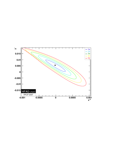
Figure 1: Confidence level of the average of the BaBar and Belle measurements of $x^{\prime 2}$ and $y^{\prime}$ (from hfagc ).

II.3 Mixing parameters from the $D\to K_{S}\,\pi^{+}\pi^{-}$ Dalitz analysis

Similar to the measurement of the CKM angle $\gamma$ from $B^{\pm}\to D(K_{S}\pi^{+}\pi^{-})K^{\pm}$, one can also search for $D^{0}$ – $\,\overline{\!D}{}{}^{0}$ mixing in the same $D$ decay. The Dalitz plot analysis is based on writing the amplitudes as

$$\langle K_{S}\pi^{+}\pi^{-}|\,{\cal H}\,|D_{0}(t)\rangle$$ (28)

$${}=A_{K_{S}\pi^{+}\pi^{-}}\big{[}e^{-(\Gamma_{1}/2+im_{1})t}+e^{-(\Gamma_{2}/2+im_{2})t}\big{]}/2$$

$${}+(q/p)\,\bar{A}_{K_{S}\pi^{+}\pi^{-}}\big{[}e^{-(\Gamma_{1}/2+im_{1})t}-e^{-(\Gamma_{2}/2+im_{2})t}\big{]}/2,$$

and similarly for $\,\overline{\!D}{}{}^{0}(t)$. Denoting $m_{\pm}=m_{K_{S}\pi^{\pm}}$, with no direct $CP$ violation, $A(m_{+},m_{-})=\bar{A}(m_{-},m_{+})$. The amplitude is modelled by a sum of resonances, $\sum_{j}a_{j}e^{i\delta_{j}}{\cal A}^{j}$, where ${\cal A}^{j}$ is the model for each resonance that depends on $m_{+}$ and $m_{-}$, while $a_{j}$ and $\delta_{j}$ are its amplitude and strong phase. Thus, the rate depends on interferences involving rapidly varying known strong phases related to the resonances (i.e., $\Gamma_{K^{*}}\ll m_{D}$), and is sensitive to $x$ and $y$, including the sign of $x/y$. With the time dependence of rates to $CP$ eigenstates (e.g., $\rho^{0}K_{S}$), all signs can be resolved (except the unphysical $\{x,\,y,\,q/p\}\to\{-x,\,-y,\,-q/p\}$).

The analysis relies on the amplitude throughout the Dalitz plot, but its modelling has only been tested with the rates so far. In the region of the Dalitz plot corresponding to large $K^{**}$ masses ($K^{**}$ denotes heavy kaon states which decay to $K_{S}\pi$) the ratio of the DCS and CF rates is significantly enhanced in the Belle model Abe:2007rd compared to that for $D\to K\pi$. While this is possible theoretically, it is less pronounced in the BaBar model Poluektov:2006ia . Data on $CP$-tagged $D\to K_{S}\pi^{+}\pi^{-}$ decays expected soon from CLEO-c could help reduce the uncertainties. (With more data, one may also attempt a model independent analysis, as for the extraction of the CKM angle $\gamma$ Giri:2003ty .)

The first significant result is from Belle Abe:2007rd

$$x=0.0080\pm 0.0034\,,\quad y=0.0033\pm 0.0028\,,$$ (29)

which is $2.7\sigma$ from the no-mixing hypothesis. The 95% CL intervals are $0<x<0.016$ and $-0.0035<y<0.010$. The preliminary result allowing for all but direct $CP$ violation (the analog of the 5-parameter fit for $K\pi$ with $A_{D}=0$, advocated above) is consistent with this result, and yields alan

$$x = 0.0081\pm 0.0034,\qquad|q/p|=0.95^{+0.22}_{-0.20}\,,$$ (30)

$$y = 0.0037\pm 0.0029,\quad\arg(q/p)=-0.03\pm 0.19,$$

where $\arg(q/p)$ is to be understood in the phase convention in which $CP\,|D^{0}\rangle=|\,\overline{\!D}{}{}^{0}\rangle$. This shows no hint of $CP$ violation yet.

II.4 Other measurements and some interpretation

Several other measurements are sensitive to $D^{0}$ – $\,\overline{\!D}{}{}^{0}$ mixing. The “wrong sign” semileptonic $D^{0}$ rate (the phenomenon by which $B^{0}$ mixing was discovered) has only quadratic sensitivity to $x$ and $y$, giving $x^{2}+y^{2}=(3.5\pm 7.7)\times 10^{-4}$ hfagc . In the limit of very large data sets, measurements with linear sensitivity are expected to give the best constraints.

Other Dalitz analyses, such as $D^{0}\to K^{+}\pi^{-}\pi^{0}$ Brandenburg:2001ze and measurements of $D^{0}\to K^{+}\pi^{-}\pi^{+}\pi^{-}$ may also prove useful in pinning down the mixing parameters by providing complementary information to the measurements discussed above.

Combining all experimental results obtained without allowing for $CP$ violation, HFAG finds a $5.7\sigma$ signal for $D^{0}$ – $\,\overline{\!D}{}{}^{0}$ mixing, with the projections hfagc

$$x=0.0087^{+0.0030}_{-0.0034}\,,\quad y=0.0066\pm 0.0021\,.$$ (31)

As the experimental uncertainties decrease, it will be interesting to allow for $CP$ violation in mixing (i.e., $|q/p|\neq 1$ and $\sin\phi\neq 0$) in the fits. If the $y$ term dominates $y_{CP}$ in Eq. (II.1) and $y^{\prime}$ dominates $y^{\prime\pm}$ in Eq. (II.2) then the $CP$ violating ratios Nir:2007ac

$${A_{\Gamma}\over y_{CP}} \approx {|q/p|^{2}-1\over|q/p|^{2}+1}-{x\over y}\tan\phi\,,$$

$${y^{\prime+}-y^{\prime-}\over y^{\prime+}+y^{\prime-}} \approx {|q/p|^{2}-1\over|q/p|^{2}+1}-{x^{\prime}\over y^{\prime}}\tan\phi\,,$$ (32)

give simple constraints on $|q/p|$ and $\phi$. This would of course be taken into account in a fit that allows $CP$ violation and includes all correlations between the measurements. While the fit assuming no $CP$ violation giving Eq. (31) has a good $\chi^{2}$, I would caution about over-interpreting it until we see how the difference between $y_{CP}$ in Eq. (II.1) and $y$ in Eq. (29) will change as the uncertainties decrease.

Given that the measured values of the $D^{0}$ – $\,\overline{\!D}{}{}^{0}$ mixing parameters may be due to long distance hadronic physics, to set constraints on new physics Ciuchini:2007cw , one has to assume that there is no cancellation between the NP and the SM contributions, and can only demand that the NP contribution does not exceed the measured values. This situation could change when $\Delta\Gamma$ and $\Delta m$ become better known, and especially if $CP$ violation is observed. Thus, it will be very interesting to robustly establish the values of the mixing parameters as more experimental results appear.

II.5 Calculations of $\Delta\Gamma_{D}$ and $\Delta m_{D}$

The reason it is notoriously hard to calculate $x$ and $y$ in the SM is that the charm quark is neither heavy nor light enough to trust the theoretical tools applicable in these two limits. The lowest order short-distance calculation of the box diagram gives tiny results,

$$x_{\rm box}\propto{m_{s}^{2}\over m_{W}^{2}}\times{m_{s}^{2}\over m_{c}^{2}}\,,\qquad y_{\rm box}\propto{m_{s}^{2}\over m_{c}^{2}}\,x_{\rm box}\,,$$ (33)

yielding few $\times 10^{-5}$ and few $\times 10^{-7}$, respectively. The $m_{s}^{4}$ suppression of $x_{\rm box}$ arises, because at short distances, above the chiral symmetry breaking scale, each power of $SU(3)$ breaking ($U$-spin breaking) required by Eq. (16) is proportional to $m_{s}^{2}$ instead of $m_{s}$ Georgi:1992as . An additional $m_{s}^{2}$ suppression of $y_{\rm box}/x_{\rm box}$ arises from the helicity suppression of the decay of a scalar meson into a massless fermion pair; this is why at leading order in the OPE, $y_{\rm box}\ll x_{\rm box}$.

Table 1: Enhancement of $\Delta m$ and $\Delta\Gamma$ relative to the box diagram (4-quark operator) at higher orders in the OPE ($\Lambda$ is a hadronic scale around 1GeV and $\beta_{0}=11-2n_{f}/3=9$).

Ratio	4-quark	6-quark	8-quark
$\displaystyle{\Delta m\over\Delta m_{\rm box}}$	1	$\displaystyle{\Lambda^{2}\over m_{s}m_{c}}$	$\displaystyle{\alpha_{s}\over 4\pi}\,\Big{(}{\Lambda^{2}\over m_{s}m_{c}}\Big{)}^{2}$
$\displaystyle{\Delta\Gamma\over\Delta m}$	$\displaystyle{m_{s}^{2}\over m_{c}^{2}}$	$\displaystyle{\alpha_{s}\over 4\pi}$	$\displaystyle\beta_{0}\,{\alpha_{s}\over 4\pi}$

It was recognized by Georgi that higher order contributions to $x$ and $y$ in the OPE have fewer powers of $m_{s}$ suppressions, since the chiral suppressions can be lifted by quark condensates instead of mass insertions Georgi:1992as . The parametric enhancement of the subleading terms are summarized in Table 1 Falk:2001hx , which shows that the 8-quark operator contributions to $x$ and $y$ are only suppressed by $m_{s}^{2}$, the minimal possible power. Thus, these higher dimension operators give the dominant contributions. Using naive dimensional analysis ($\Lambda\sim 4\pi f_{\pi}$) and different assumptions to estimate the matrix elements, one can find smaller Ohl:1992sr or larger enhancements Bigi:2000wn , yielding up to

$$x\sim y\sim 10^{-3}\,.$$ (34)

Since there are several unknown matrix elements which are hard to estimate, these results are at best useful to understand the orders of magnitudes of $x$ and $y$, but not for obtaining reliable SM predictions (even at the factor of 2–3 level).

In a long-distance analysis, instead of assuming that the $D$ meson is heavy enough for duality to hold between the partonic rate and the sum over hadronic final states, one examines certain exclusive decay modes. There is a contribution to $y$ from all final states common to $D^{0}$ and $\,\overline{\!D}{}{}^{0}$ decay,

$$y={\sum_{n}\rho_{n}\langle\,\overline{\!D}{}{}^{0}|\,{\cal H}_{w}|n\rangle\langle n|\,{\cal H}_{w}|D^{0}\rangle\over\sum_{n}\Gamma(D^{0}\to n)}\,,$$ (35)

where $\rho_{n}$ is the phase space available to the state $n$ (we neglect $CP$ violation, and choose $\Gamma_{12}$ to be real). We denote by $y_{F,R}$ the expression in Eq. (35) with the sum over $n$ restricted to states $F$ (e.g., certain number of pseudoscalar or vector mesons) in the $SU(3)$ representation $R$, $n\in F_{R}$. The $y_{F,R}$ are the “would-be” values of $y$, if $D$ only decayed to $F_{R}$. In the $SU(3)$ limit, $y_{F,R}=0$. Since $D$ decays are not dominated by a few final states and there are cancellations between states within a given $SU(3)$ multiplet, to make a reliable estimate one would need to know the contributions of many states with high precision. In the absence of sufficiently precise data on the rates and strong phases, one has to use assumptions.

The importance of $SU(3)$ cancellations in the magnitudes and phases of matrix elements can be illustrated by $D$ decays to a pair of charged $\pi$’s and $K$’s. The $SU(3)$ breaking is very large in ${\cal B}(D^{0}\to K^{+}K^{-})/{\cal B}(D^{0}\to\pi^{+}\pi^{-})\approx 2.8$, which is unity in the $SU(3)$ limit. This was the basis for the claim that $SU(3)$ is not applicable to $D$ decays, so $x,y\sim 10^{-2}$ is possible Wolfenstein:1985ft . (However, as we show below, these states alone are unlikely to give so large $x$ and $y$, due to their small rates.) The value of $y$ corresponding to decays to $\pi^{+}\pi^{-}$, $\pi^{\pm}K^{\mp}$, and $K^{+}K^{-}$ is

$$y_{\pi K} \propto {\cal B}(D^{0}\to\pi^{+}\pi^{-})+{\cal B}(D^{0}\to K^{+}K^{-})$$

$$- 2\cos\delta\,\sqrt{{\cal B}(D^{0}\to K^{-}\pi^{+})\,{\cal B}(D^{0}\to K^{+}\pi^{-})}\,,$$

where $\delta$ is the strong phase between the CF and DCS amplitudes defined after Eq. (19), which vanishes in the $SU(3)$ limit. The experimental central values pdg yield $(5.2-4.7\cos\delta)\times 10^{-3}$. For small $\delta$, there is a significant cancellation, and the result is consistent with zero within $1\sigma$, even though the individual rates badly violate $SU(3)$. One cannot use, however, this exclusive approach to reliably predict $x$ or $y$, since the estimates are very sensitive to $SU(3)$ breaking in poorly known strong phases and DCS rates.

The cancellations that give $y_{F,R}=0$ in the $SU(3)$ limit depend on both the matrix elements and the phase space, $\rho_{n}$, in Eq. (35). We cannot estimate model independently the $SU(3)$ violation in matrix elements, but that in the phase space is calculable, as it mainly depends on the hadron masses in the final states, and can be computed with mild assumptions about the momentum dependence of the matrix elements. Incorporating the true values of $\rho_{n}$ in Eq. (35) is a calculable source of $SU(3)$ breaking. This contribution to $y$ due to $SU(3)$ violation in phase space is negligible for two-body pseudoscalar final states, but can be of the order of a percent for final states with masses near $m_{D}$.

To illustrate some aspects of this analysis Falk:2001hx ; Ligeti:2002gc , consider the above example of the $U$-spin doublet of charged kaons and pions,

$$y_{\pi K} = \sin^{2}\theta_{C}\,\big{[}\Phi(\pi^{+},\pi^{-})+\Phi(K^{+},K^{-})$$ (37)

$${}-2\Phi(K^{+},\pi^{-})\big{]}\,\big{/}\,\Phi(K^{+},\pi^{-})\,,$$

where $\Phi$ is the phase space. This model sets $\delta=0$, so it gives $y_{\pi K}\sim-0.01\sin^{2}\theta_{C}$, a tiny result. For representations in which some states are not allowed by phase space, $SU(3)$ breaking is large. For example, for 4 pseudoscalar mesons the phase space depends very strongly on the number of kaons and vanishes for $D\to 4K$ ($m_{4K}>m_{D}$), giving $y_{4P}={\cal O}(\sin^{2}\theta_{C})$. Clearly, this enhancement of $y$ is a “threshold effect”, which would be small if $m_{c}$ were heavier, but is significant for the physical value of $m_{c}$. Not all final states which may give large contributions were considered in Ref. Falk:2001hx ; e.g., ${\cal B}(D^{0}\to K^{-}a_{1}^{+})=(7.5\pm 1.1)\%$, although its phase space is very small. Since 4 pseudoscalars account for $\sim$10% of the $D$ width, the contribution of these states alone to $y$ can be near 0.01.

Thus, we conclude that $y\sim 0.01$ is natural in the SM. An order of magnitude smaller result would require significant cancellations, which would only be expected if they were enforced by the OPE.

To connect the calculation of $y$ to $x$, a dispersion relation can be proven in HQET, which relates $\Delta m$ to an integral of $\Delta\Gamma$ over the mass $M$ of a heavy “would-be $D$ meson” Falk:2004wg

$$\Delta m=-\frac{1}{2\pi}\,{\rm P}\!\int_{2m_{\pi}}^{\infty}{\rm d}M\,\frac{\Delta\Gamma(M)}{M-m_{D}}+\ldots\,.$$ (38)

Modelling that phase space is the only source of $SU(3)$ breaking, the calculation of $x$ based on this relation is more model dependent than that of $y$. Unlike the estimate of $y$, the hadronic matrix elements do not cancel in $x$, since some assumptions about the $M$-dependence of the rates has to be made. The most significant (tractable) contributions come again from 4-body final states, which can give $x$ comparable in magnitude to $y$ (thought typically $0.1<x/y\lesssim 1$) Falk:2004wg .

II.6 Summary for $D^{0}$ – $\,\overline{\!D}{}{}^{0}$ mixing

• The central values of recent experimental results may be due to SM physics.

• It is possible that $\Delta\Gamma/(2\Gamma)\sim 0.01$ in the SM (some calculable contributions are of this size).

• It is likely that $\Delta m\lesssim\Delta\Gamma$ in the SM (though this relies on significant assumptions).

• If $x<y$ then sensitivity to NP is reduced, even if NP dominates $M_{12}$.

• The SM predictions of $\Delta m$ and $\Delta\Gamma$ remain uncertain, so their measurements alone (especially if $\Delta m\lesssim\Delta\Gamma$) cannot be interpreted as NP.

• It is important to improve the constraints on both $\Delta\Gamma$ and $\Delta m$, and to look for $CP$ violation, which remains a potentially robust signal of NP.

III $B_{s}^{0}$ – $\,\overline{\!B}{}{}^{0}_{s}$ mixing

The $B_{s}^{0}$ and $\,\overline{\!B}{}{}^{0}_{s}$ mesons oscillate about 25 times before they decay, which made measuring the oscillation frequency very challenging. The measurement Abulencia:2006ze

$$\Delta m_{s}=(17.77\pm 0.10\pm 0.07)\,{\rm ps}^{-1}\,,$$ (39)

is a key to test and overconstrain the CKM matrix and the SM description of $CP$ violation. Amusingly, the experimental uncertainty $\sigma(\Delta m_{s})=0.7\%$ is already smaller than $\sigma(\Delta m_{d})=0.8\%$, which has been measured for over 20 years.

To interpret the result in Eq. (39) in terms of CKM parameters, the largest uncertainty comes from the hadronic matrix element $f_{B_{s}}\sqrt{B_{s}}$, whose error is around 15%. To reduce this (and because in the context of testing the SM one is more interested in the value of $|V_{td}V_{tb}|$ than $|V_{ts}V_{tb}|$), one considers the ratio $\Delta m_{s}/\Delta m_{d}$, which is precisely calculable in terms of $|V_{td}/V_{ts}|$ and $\xi=(f_{B_{s}}\sqrt{B_{s}})/(f_{B_{d}}\sqrt{B_{d}})$. Here $\xi$ quantifies $SU(3)$-breaking corrections to the ratio of matrix elements, which can be calculated more accurately in lattice QCD (LQCD) than the matrix elements separately (the calculation of chiral logs predicts $\xi\sim 1.2$ Bslogs ). CDF infers from its measurement of $\Delta m_{s}$ the ratio of CKM elements,

$$|V_{td}/V_{ts}|=0.206\pm 0.001\mbox{(exp)}\,^{+0.008}_{-0.006}\mbox{(theo)}\,,$$ (40)

where the error is dominated by the theoretical uncertainty of $\xi=1.21^{+0.047}_{-0.035}$ Okamoto:2005zg , used by CDF. The CDF, DØ, ALEPH, and DELPHI experiments have also measured the $B_{s}^{0}$ lifetimes in $CP$-even, $CP$-odd, and flavor specific final states, yielding hfag

$$\Delta\Gamma_{s}^{CP}=(0.071^{+0.053}_{-0.057})\,{\rm ps}^{-1},$$ (41)

where $\Delta\Gamma_{s}^{CP}=\Gamma_{CP+}-\Gamma_{CP-}=-\cos\phi_{12}\,\Delta\Gamma_{s}$ Grossman:1996er ; Dunietz:2000cr . This is similar to the measurement of $y_{CP}$ in Sec. II.1.

The mixing in the $B_{d}$ and $B_{s}$ systems are short distance dominated, so the theory errors in interpreting $\Delta m_{d,s}$ are suppressed compared to the measured values. (This is in contrast with $\Delta m_{D}$ and $\epsilon^{\prime}/\epsilon$, where due to hadronic uncertainties we only know at present that the NP contributions do not exceed the observations.) The interpretation of the measurement of $\Delta\Gamma_{s}^{CP}$ (or $\Delta\Gamma_{s}$) relies on the calculation of $\Gamma_{12}$, which is on the same footing as that of heavy hadron lifetimes. This makes it important to resolve whether the “$\Lambda_{b}$ lifetime problem” is a theoretical or an experimental one (i.e., theory predicts $\tau_{\Lambda_{b}}/\tau_{B_{s}}\sim 0.9$, while the world average is about 0.8, except a recent CDF measurement giving a ratio near 1).

To discuss possible NP contributions, we concentrate on NP in $\Delta F=2$ processes and assume that (i) the $3\times 3$ CKM matrix is unitary and (ii) tree-level decays are SM dominated Soares:1992xi . Then there are two new parameters for each meson mixing amplitude

$$M_{12}=\,\underbrace{M_{12}^{\rm SM}\,r_{s}^{2}\,e^{2i\theta_{s}}}_{{\rm easy~{}to~{}relate~{}to~{}data}}\,\equiv\,\underbrace{M_{12}^{\rm SM}\big{(}1+h_{s}\,e^{2i\sigma_{s}}\big{)}}_{\rm easy~{}to~{}relate~{}to~{}NP}.$$ (42)

We use the $h,\sigma$ parameterization, since any NP model would give an additive contribution to $M_{12}$. To constrain $h$ and $\sigma$, the measurements of $|V_{ub}/V_{cb}|$ and $\gamma$ (or $\pi-\beta-\alpha$) that come from tree-level processes and are therefore unaffected by the NP are crucial Ligeti:2004ak . One can then compare these with the $B\,\overline{\!B}{}$ mixing dependent observables sensitive to $h$ and $\sigma$, which include $\Delta m_{d,s}$, $S_{f_{i}}$, $A_{\rm SL}^{d,s}$, $\Delta\Gamma_{s}^{CP}$. (As mentioned above, the hadronic uncertainties are sizable in $A_{\rm SL}^{d,s}$ and $\Delta\Gamma_{s}^{CP}$, but in the SM $A_{\rm SL}^{d,s}\ll$ current bound, while for $\Delta\Gamma_{s}^{CP}$ they are comparable. If hadronic uncertainties are treated conservatively, improving the measurement of $\Delta\Gamma_{s}^{CP}$ will not yield a better constraint unless LQCD determines the bag parameters with smaller errors, while the bound from $A_{\rm SL}^{d,s}$ will improve independent of progress in LQCD.)

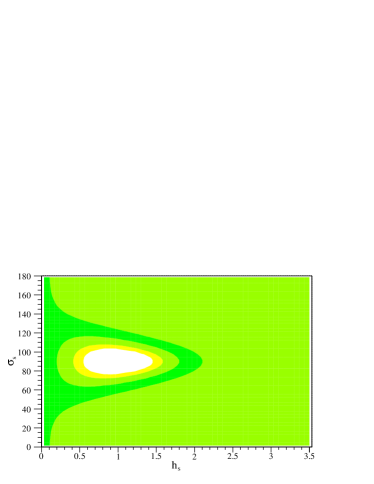
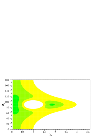
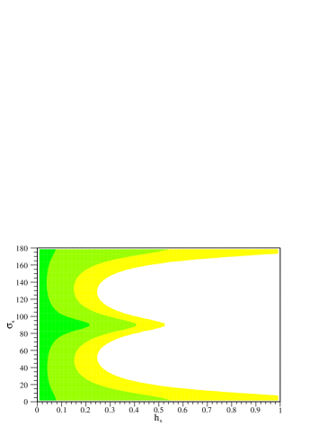
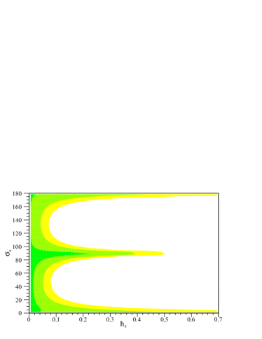
Figure 2: Constraints on $h_{s}$ and $\sigma_{s}$ before (top left) and after (top right) the $\Delta m_{s}$ and $\Delta\Gamma_{s}^{CP}$ measurements. The second row (note the different scales) shows the impact of a future masurement of $S_{\psi\phi}$ with $\sigma(S_{\psi\phi})=0.1$ (bottom left) and $0.03$ (bottom right), expected after 0.1 yr and 1 yr of nominal LHCb data. The dark green, light green, and yellow areas have CL $>$ 0.90, 0.32, and 0.05, respectively, indicating the theory uncertainty, $1\sigma$, and $2\sigma$ regions (from Ligeti:2006pm ).

The NP parameters modify the SM predictions as

$$\Delta m_{s} = \Delta m_{s}^{\rm SM}\,\big{|}1+h_{q}e^{2i\sigma_{q}}\big{|},$$

$$\Delta\Gamma_{s}^{CP} = |\Delta\Gamma_{s}^{\rm SM}|\,\cos^{2}\!\big{[}\arg\big{(}1+h_{s}e^{2i\sigma_{s}}\big{)}\big{]}.$$ (43)

The top row in Fig. 2 shows the constraint on $h_{s}$ and $\sigma_{s}$ before (left) and after (right) the Tevatron measurements of $\Delta m_{s}$ and $\Delta\Gamma_{s}^{CP}$. To further restrict the parameter space, one needs measurements sensitive to the $CP$ violating phase in $B_{s}$ mixing, which will come from $S_{\psi\phi}$, the time dependent $CP$ asymmetry in $B_{s}\to J/\psi\,\phi$. This is the analog of $S_{\psi K}=\sin 2\beta$ in $B_{d}\to J/\psi K_{S}$. In the SM, $S_{\psi\phi}=\sin 2\beta_{s}$ for the $CP$-even part of the final state, where

$$\beta_{s}=\arg(-V_{ts}V_{tb}^{*}/V_{cs}V_{cb}^{*})={\cal O}(\lambda^{2})\,,$$ (44)

is the small angle in one of the “squashed” unitarity triangles, for which the CKM fit predicts $\sin 2\beta_{s}=0.0365^{+0.0021}_{-0.0020}$ ckmfitter . In the presence of NP

$$S_{\psi\phi}=\sin\!\big{[}2\beta_{s}-\arg\big{(}1+h_{s}e^{2i\sigma_{s}}\big{)}\big{]}.$$ (45)

Just like when the first $B$ factory results emerged in 2000 the first question was whether $\sin 2\beta$ was consistent with the constraints at that time (mainly from $\epsilon_{K}$, $|V_{ub}/V_{cb}|$, and $\Delta m_{B}$), in 2009 the question will be if the first measurements of $\sin 2\beta_{s}$ are consistent with its smallness predicted by the SM. It is not necessary to measure it with a sensitivity near the SM to make a significant impact, and CDF or DØ may also be able to do a first measurement Anikeev:2001rk ; Abazov:2007zj . Observing a sizable nonzero value of $S_{\psi\phi}$ would disprove both the SM and minimal flavor violation (MFV) scenarios.

The plots in the second row in Fig. 2 show the constraints on $h_{s}$ and $\sigma_{s}$ when the measurement of $S_{\psi\phi}$ will be available with an error of 0.1 (left) and 0.03 (right), which are expected with 0.1 and 1 year of nominal LHCb data. Such a relatively small data set will constrain $h_{s}$ below $0.1$, except if $\sigma_{s}$ is near 0 (mod $\pi/2$), where significant deviations from the SM will still be allowed, but only in a way consistent with MFV. These two plots do not contain a constraint from $\Delta\Gamma_{s}^{CP}$, which may be dominated by hadronic uncertainties by that time.

The parameter $h$ gives some measure of “fine tuning”. We expect generically $h\sim(4\pi v/\Lambda)^{2}$, so as long as $h\sim 1$ is allowed, the flavor scale can be $\Lambda_{\rm flavor}\sim 2\,{\rm TeV}\sim\Lambda_{\rm EWSB}$, while if future data constrain $h<0.1$ then $\Lambda_{\rm flavor}>7\,{\rm TeV}\gg\Lambda_{\rm EWSB}$. If NP is seen at the LHC and the constraints on the flavor scale are pushed up near 10 TeV, i.e., if $h<0.1$ can be achieved, we shall know that some additional mechanism is present suppressing FCNC’s.

Another interesting observable which can constrain NP Laplace:2002ik , and has recently been started to be constrained experimentally is $A_{\rm SL}^{d,s}$,

$$A_{\rm SL}(t) = {\Gamma[\,\overline{\!B}{}^{0}(t)\to\ell^{+}X]-\Gamma[B^{0}(t)\to\ell^{-}X]\over\Gamma[\,\overline{\!B}{}^{0}(t)\to\ell^{+}X]+\Gamma[B^{0}(t)\to\ell^{-}X]}$$ (46)

$$= {1-|q/p|^{4}\over 1+|q/p|^{4}}\approx 2\big{(}1-|q/p|\big{)},$$

which is actually time-independent, and measures the difference between the $B\to\,\overline{\!B}{}$ and $\,\overline{\!B}{}\to B$ probabilities old . In the SM, $A_{\rm SL}^{s}\sim 3\times 10^{-5}$ Beneke:2003az is unobservably small. In $K$ decay the similar asymmetry has been measured cplear , in agreement with the expectation that it is $4\,{\rm Re}\,\epsilon$. In the presence of NP Ligeti:2006pm ; Blanke:2006ig ; Grossman:2006ce

$$A^{s}_{\rm SL}={\rm Im}\big{\{}\Gamma_{12}^{s}/\big{[}M_{12}^{s,{\rm SM}}(1+h_{s}e^{2i\sigma_{s}})\big{]}\big{\}}.$$ (47)

Figure 3 shows the allowed region of $A^{s}_{\rm SL}$ as a function of $h_{s}$. Interestingly, $A^{s}_{\rm SL}$ can still be as much as ${\cal O}(10^{3})$ times its SM value, and $|A_{\rm SL}^{s}|>|A_{\rm SL}^{d}|$ is possible, contrary to the SM.

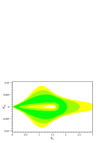
Figure 3: Allowed region of $A_{\rm SL}^{s}$ and $h_{s}$ (from Ligeti:2006pm ).

Due to the smallness of $\beta_{s}$ in the SM, $A_{\rm SL}^{s}$ and $S_{\psi\phi}$ are strongly correlated in the region of NP parameter space in which $h_{s},\sigma_{s}\gg\beta_{s}$ Ligeti:2006pm

$$A_{\rm SL}^{s}=-\left|\Gamma^{s}_{12}\over M^{s}_{12}\right|^{\rm SM}S_{\psi\phi}+{\cal O}\bigg{(}h_{s}^{2},\,{m_{c}^{2}\over m_{b}^{2}}\bigg{)}.$$ (48)

This correlation, which holds in any model where NP does not affect tree level processes, is plotted in Fig. 4, including theoretical uncertainties. Should the measured values violate this correlation, we would know that NP cannot be parameterized simply by Eq. (42).

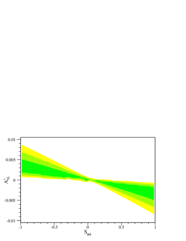
Figure 4: Correlation between $A_{\rm SL}^{s}$ and $S_{\psi\phi}$ (from Ligeti:2006pm ).

III.1 Summary for $B_{s}^{0}$ – $\,\overline{\!B}{}{}^{0}_{s}$ mixing

• Measurements at the Tevatron started to constrain new physics in $\Delta F=2$ $b\to s$ transitions.

• Nevertheless, significant non-SM contributions are still allowed.

• To make progress, measurements of $S_{\psi\phi}$ and $A_{\rm SL}^{s}$ are needed (but sensitivity at the SM level is not required to have important implications).

• LHCb can distinguish between MFV and non-MFV scenarios (observation of $S_{\psi\phi}\neq 0$ at the Tevatron would rule out the SM and MFV).

• If evidence for NP is found, the correlation of $S_{\psi\phi}$ and $A_{\rm SL}^{s}$ may help to understand its nature.

Table 2: SM expectations and measurements of $x$ and $y$ (neglecting $CP$ violation in mixing), and $(1-|q/p|^{4})/(1+|q/p|^{4})$.

$x=\Delta m/\Gamma$ $y=\Delta\Gamma/(2\Gamma)$ $A=(1-|q/p|^{4})/(1+|q/p|^{4})$ SM theory data SM theory data SM theory data $B_{d}$ ${\cal O}(1)$ $0.775$ $y_{s}\,|V_{td}/V_{ts}|^{2}$ $-0.005\pm 0.019$ $-(5.5\pm 1.5)10^{-4}$ $(-4.7\pm 4.6)\!\times\!10^{-3}$ $B_{s}$ $x_{d}\,|V_{ts}/V_{td}|^{2}$ $25.8$ ${\cal O}(-0.1)$ $-0.05\pm 0.04$ $-A_{d}\,|V_{td}/V_{ts}|^{2}$ $(0.3\pm 9.3)\!\times\!10^{-3}$ $K$ ${\cal O}(1)$ $0.948$ $-1$ $-0.998$ $4\,{\rm Re}\,\epsilon$ $(6.6\pm 1.6)\!\times\!10^{-3}$ $D$ $\lesssim 0.01$ $<0.016$ (95% CL) ${\cal O}(0.01)$ $0.011\pm 0.003$ ($y_{CP}$) $<10^{-4}$ ${\cal O}(0.5)$ bound only

IV Concluding remarks

Instead of a usual summary, Table 2 shows the SM predictions and the current experimental information on the mixing parameters, $x=\Delta m/\Gamma$, $y=\Delta\Gamma/(2\Gamma)$, and $A=(1-|q/p|^{4})/(1+|q/p|^{4})$. While $|q/p|$ is very near 1 in the $K^{0}$, $B_{d}^{0}$, and $B_{s}^{0}$ systems, we do not know this for the $D^{0}$ yet (it does hold in the SM). The correspondence between the lifetimes, $CP$ eigenstates, and mass eigenstates of the neutral mesons, in the limit neglecting $CP$ violation, is

$$K\!\! : \mbox{long-lived}=CP\mbox{-odd}=\mbox{heavy},$$ (49)

$$D\! : \mbox{long-lived}=CP\mbox{-odd }(3.5\sigma)=\mbox{light }(2\sigma),$$

$$B_{s}\!\! : \mbox{long-lived}=CP\mbox{-odd }(1.5\sigma)=\mbox{heavy in the SM},$$

$$B_{d}\!\! : \mbox{yet unknown; same as $B_{s}$ in SM for $m_{b}\!\gg\!\Lambda_{\rm QCD}$}.$$

Taking Belle’s $D\to K_{S}\pi^{+}\pi^{-}$ analysis as evidence for the sign of $x/y$ implies that the $CP$-odd $D^{0}$ state is the lighter one, contrary to the $K^{0}$ system (and probably the $B_{d,s}$ systems as well). This information is more amusing than useful, since it does not tell us which measurements give clean short-distance information.  Curiously, before 2006 we only knew experimentally the first line in (49).

As an aside, note that in the $B_{d}^{0}$ system it is hard, if not impossible, to identify the $CP$-even and odd states simply by their decays to $CP$ eigenstates. Although $B_{L,H}$ can be defined as almost pure $CP$ eigenstates, both $B_{L,H}$ can decay to the same $CP$ eigenstates, since the weak interaction responsible for the decays does not conserve $CP$. If the phase of the decay and the mixing amplitudes are not the same ($V_{tb}V_{td}^{*}$), i.e., if $\lambda\neq\pm 1$, then the untagged $B$ decay rate is

$$\Gamma(B\to f) \propto \left(1+{2\,{\rm Re}\,\lambda\over 1+|\lambda|^{2}}\right)e^{-\Gamma_{L}t}$$ (50)

$$+ \left(1-{2\,{\rm Re}\,\lambda\over 1+|\lambda|^{2}}\right)e^{-\Gamma_{H}t}\,,$$

indicating that both $B_{H}$ and $B_{L}$ can decay to the same final $CP$ eigenstate. It is not yet known if $CP$ violation is absent in any decay to a $CP$ eigenstate. It would be if $b\to d$ penguins (e.g., $B\to\phi\pi^{0}$) were dominated by the top loop, however, the $V_{tb}V_{td}^{*}$ and $V_{cb}V_{cd}^{*}$ terms are comparable. The best hope, in principle, may be $B\to\rho^{+}\rho^{-}$, if the data converge toward $\alpha$ near $90^{\circ}$ and small penguin to tree ratio.

Looking into the future, some of the most interesting measurements which I hope will emerge are as follows. In $D^{0}$ – $\,\overline{\!D}{}{}^{0}$ mixing:

• More robust measurements of $\Delta m$ and $\Delta\Gamma$;

• Will CPV be observed?  Is $|q/p|$ near 1?

• Result of $K\pi$ fit with $5$ parameters (allowing $CP$ violation in mixing, but not in decay).

In $B_{s}^{0}$ – $\,\overline{\!B}{}{}^{0}_{s}$ mixing:

• Better constraint on / measurement of $S_{\psi\phi}$;

• Improved bounds on $A_{\rm SL}$;

• Better lattice QCD results for $\Delta m$ and $\Delta\Gamma$.

Clearly, we can learn a lot from these measurements, so it will be exciting to see what they teach us over the next several years. Either new physics signals may be observed, or the flavor structure of the SM will have been tested (or that of the NP seen at the LHC constrained) at a whole new level, providing insights to the physics of flavor changing interactions.

- (1) A. Abulencia et al. [CDF Collaboration], Phys. Rev. Lett. 97, 242003 (2006) [hep-ex/0609040].
- (2) B. Aubert et al. [BaBar Collaboration], Phys. Rev. Lett. 98, 211802 (2007) [hep-ex/0703020].
- (3) M. Staric et al. [Belle Collaboration], Phys. Rev. Lett. 98, 211803 (2007) hep-ex/0703036.
- (4) M. Papucci, talk at this conference, http://www-f9.ijs.si/fpcp07/.
- (5) B. Grinstein, talk at this conference, http://www-f9.ijs.si/fpcp07/.
- (6) K. Agashe, M. Papucci, G. Perez and D. Pirjol, hep-ph/0509117; and references therein.
- (7) Y. Nir and N. Seiberg, Phys. Lett. B 309, 337 (1993) [hep-ph/9304307].
- (8) See, e.g., G. C. Branco, L. Lavoura and J. P. Silva, CP Violation, International Series of Monographs on Physics, Clarendon Press, Oxford, UK (1999).
- (9) Y. Grossman, Phys. Lett. B 380, 99 (1996) [hep-ph/9603244].
- (10) S. Bergmann, Y. Grossman, Z. Ligeti, Y. Nir and A. A. Petrov, Phys. Lett. B 486, 418 (2000) [hep-ph/0005181].
- (11) A. F. Falk, Y. Grossman, Z. Ligeti and A. A. Petrov, Phys. Rev. D 65, 054034 (2002) [hep-ph/0110317].
- (12) E. Golowich, S. Pakvasa and A. A. Petrov, hep-ph/0610039.
- (13) E. Barberio et al. [Heavy Flavor Averaging Group (HFAG)], http://www.slac.stanford.edu/xorg/hfag/charm/.
- (14) B. Aubert et al. [BaBar Collaboration], Phys. Rev. Lett. 91, 121801 (2003) [hep-ex/0306003]; S. E. Csorna et al. [CLEO Collaboration], Phys. Rev. D 65, 092001 (2002) [hep-ex/0111024]; J. M. Link et al. [FOCUS Collaboration], Phys. Lett. B 485, 62 (2000) [hep-ex/0004034]; E. M. Aitala et al. [E791 Collaboration], Phys. Rev. Lett. 83, 32 (1999) [hep-ex/9903012].
- (15) L. M. Zhang et al. [Belle Collaboration], Phys. Rev. Lett. 96, 151801 (2006) [hep-ex/0601029].
- (16) R. Godang et al. [CLEO Collaboration], Phys. Rev. Lett. 84, 5038 (2000) [hep-ex/0001060]; J. M. Link et al. [FOCUS Collaboration], Phys. Lett. B 618, 23 (2005) [hep-ex/0412034].
- (17) A. Schwartz, talk at this conference, http://www-f9.ijs.si/fpcp07/.
- (18) G. W. Meisner, B. B. Crawford, and F. S. Crawford, Phys. Rev. Lett. 17, 492 (1966); J. Canter et al., Phys. Rev. Lett. 17, 942 (1966); J. V. Jovanovich et al., Bull. Am. Phys. Soc. 11, 469 (1996); O. Piccioni et al., Bull. Am. Phys. Soc. 11, 767 (1996).
- (19) K. Abe et al. [Belle Collaboration], arXiv:0704.1000 [hep-ex].
- (20) A. Poluektov et al. [Belle Collaboration], Phys. Rev. D 73, 112009 (2006) [hep-ex/0604054]; B. Aubert et al. [BaBar Collaboration], hep-ex/0607104; compare Tables 1 in these or in Abe:2007rd .
- (21) A. Giri, Y. Grossman, A. Soffer and J. Zupan, Phys. Rev. D 68, 054018 (2003) [hep-ph/0303187].
- (22) G. Brandenburg et al. [CLEO Collaboration], Phys. Rev. Lett. 87, 071802 (2001) [hep-ex/0105002]; X. C. Tian et al. [Belle Collaboration], Phys. Rev. Lett. 95, 231801 (2005) [hep-ex/0507071]; B. Aubert et al. [BaBar Collaboration], Phys. Rev. Lett. 97, 221803 (2006) [hep-ex/0608006].
- (23) Y. Nir, JHEP 0705 (2007) 102 [hep-ph/0703235].
- (24) M. Ciuchini et al., hep-ph/0703204; E. Golowich, J. Hewett, S. Pakvasa and A. A. Petrov, arXiv:0705.3650 [hep-ph]; and references therein.
- (25) H. Georgi, Phys. Lett. B 297, 353 (1992) [hep-ph/9209291].
- (26) T. Ohl, G. Ricciardi and E. H. Simmons, Nucl. Phys. B 403, 605 (1993) [hep-ph/9301212].
- (27) I. I. Y. Bigi and N. G. Uraltsev, Nucl. Phys. B 592, 92 (2001) [hep-ph/0005089].
- (28) M. J. Savage, Phys. Lett. B 257, 414 (1991).
- (29) L. Wolfenstein, Phys. Lett. B 164, 170 (1985).
- (30) W. M. Yao et al. [Particle Data Group], J. Phys. G 33, 1 (2006).
- (31) Z. Ligeti, AIP Conf. Proc. 618, 298 (2002) [hep-ph/0205316].
- (32) Z. Ligeti, I. W. Stewart and M. B. Wise, Phys. Lett. B 420, 359 (1998) [hep-ph/9711248].
- (33) S. Nussinov and M. V. Purohit, Phys. Rev. D 65, 034018 (2002) [hep-ph/0108272].
- (34) A. F. Falk, Y. Grossman, Z. Ligeti, Y. Nir and A. A. Petrov, Phys. Rev. D 69, 114021 (2004) [hep-ph/0402204].
- (35) B. Grinstein et al., Nucl. Phys. B 380 (1992) 369 [hep-ph/9204207].
- (36) M. Okamoto, PoS LAT2005, 013 (2006) [hep-lat/0510113].
- (37) E. Barberio et al. [Heavy Flavor Averaging Group (HFAG)], arXiv:0704.3575 [hep-ex]; updates at http://www.slac.stanford.edu/xorg/hfag/.
- (38) I. Dunietz, R. Fleischer and U. Nierste, Phys. Rev. D 63, 114015 (2001) [hep-ph/0012219].
- (39) J. M. Soares and L. Wolfenstein, Phys. Rev. D 47, 1021 (1993); T. Goto, N. Kitazawa, Y. Okada and M. Tanaka, Phys. Rev. D 53, 6662 (1996) [hep-ph/9506311]; J. P. Silva and L. Wolfenstein, Phys. Rev. D 55, 5331 (1997) [hep-ph/9610208]; Y. Grossman, Y. Nir and M. P. Worah, Phys. Lett. B 407, 307 (1997) [hep-ph/9704287].
- (40) Z. Ligeti, Int. J. Mod. Phys. A 20, 5105 (2005) [hep-ph/0408267]; UTfit Collaboration (M. Bona et al.), JHEP 0603, 080 (2006) [hep-ph/0509219]; F. J. Botella, G. C. Branco, M. Nebot and M. N. Rebelo, Nucl. Phys. B 725, 155 (2005) [hep-ph/0502133].
- (41) Z. Ligeti, M. Papucci and G. Perez, Phys. Rev. Lett. 97, 101801 (2006) [hep-ph/0604112];
- (42) A. Hocker, H. Lacker, S. Laplace and F. Le Diberder, Eur. Phys. J. C 21 (2001) 225 [hep-ph/0104062]; J. Charles et al., Eur. Phys. J. C 41 (2005) 1 [hep-ph/0406184]; and updates at http://ckmfitter.in2p3.fr/.
- (43) K. Anikeev et al., “ physics at the Tevatron: Run II and beyond,” hep-ph/0201071 (2002).
- (44) V. M. Abazov et al. [DØ Collaboration], hep-ex/0702030.
- (45) S. Laplace, Z. Ligeti, Y. Nir and G. Perez, Phys. Rev. D 65 (2002) 094040 [hep-ph/0202010]; L. Randall and S. f. Su, Nucl. Phys. B 540, 37 (1999) [hep-ph/9807377]; R. N. Cahn and M. P. Worah, Phys. Rev. D 60, 076006 (1999) [hep-ph/9904480].
- (46) J. S. Hagelin, Nucl. Phys. B 193, 123 (1981); A. J. Buras, W. Slominski and H. Steger, Nucl. Phys. B 245, 369 (1984).
- (47) M. Beneke, G. Buchalla, A. Lenz and U. Nierste, Phys. Lett. B 576 (2003) 173 [hep-ph/0307344]; M. Ciuchini et al., JHEP 0308 (2003) 031 [hep-ph/0308029].
- (48) A. Angelopoulos et al. [CPLEAR Collaboration], Phys. Lett. B 444 (1998) 43.
- (49) M. Blanke, A. J. Buras, D. Guadagnoli and C. Tarantino, JHEP 0610, 003 (2006) [hep-ph/0604057].
- (50) Y. Grossman, Y. Nir and G. Raz, Phys. Rev. Lett. 97, 151801 (2006) [hep-ph/0605028];