QMUL-PH-07-10

We discuss the calculation of one-loop amplitudes in ${\cal N}\!=\!8$ supergravity using MHV diagrams. In contrast to MHV amplitudes of gluons in Yang-Mills, tree-level MHV amplitudes of gravitons are not holomorphic in the spinor variables. In order to extend these amplitudes off shell, and use them as vertices to build loops, we introduce certain shifts for the spinor variables associated to the loop momenta. Using this off-shell prescription, we rederive the four-point MHV amplitude of gravitons at one loop, in complete agreement with known results. We also discuss the extension to the case of one-loop MHV amplitudes with an arbitrary number of gravitons.

1 Introduction

Over the past years, several new techniques in perturbative quantum field theory have emerged, following Witten’s proposal that weakly-coupled Yang-Mills theory can be equivalently described by a twistor string theory [1] (see [2] for a review). The first twistor-inspired realisation of a diagrammatic method alternative to Feynman diagrams is the MHV diagram method introduced by Cachazo, Svrček and Witten (CSW) in [3]. In that paper, it was proposed that MHV scattering amplitudes of gluons appropriately continued off the mass shell, can be used as vertices, to be joined with scalar propagators, in a novel perturbative expansion of Yang-Mills theory. The proposal of CSW, originally applied to amplitudes at tree level, was strongly supported by the study of the multi-particle singularities of the amplitudes, which are neatly reproduced by a calculation based on MHV diagrams. Shortly after, several old and new amplitudes at tree level were computed in [4, 5, 6, 7], also with fermions and scalars on the external legs.

A key ingredient of the CSW approach is the introduction of an off-shell continuation of the Parke-Taylor formula for the MHV amplitude of gluons, which is necessary in order to lift the amplitude to a full-fledged vertex. This off-shell continuation, which we will discuss in the following sections, is based on a decomposition of momenta identical to that used in lightcone quantisation of Yang-Mills, where a generic momentum $L$ is written as $L=l+z\eta$. Here $\eta_{\alpha\dot{\alpha}}:=\eta_{\alpha}\tilde{\eta}_{\dot{\alpha}}$ is an arbitrary null vector determining a lightlike direction, and $l$ is also null. This resemblance is not accidental – indeed, it was shown in [8] (see also [9]) that a particular change of variables in the lightcone Yang-Mills path integral leads to a new action for the theory with an infinite number of MHV vertices. Mansfield used the holomorphicity of the MHV amplitudes of gluons to argue that the new vertices are precisely given by the Parke-Taylor formula continued off shell as proposed in [3]. This was also checked explicitly for the four- and five-point vertices in [10]. The same off-shell prescription was also recently seen to emerge from twistor actions in an axial gauge in [11].

Although initially limited to Yang-Mills theory, progress has also been made in other theories, specifically in gravity. This includes applications of the BCF recursion relation [12, 13] to amplitudes of gravitons, [14, 15, 16, 17], and (generalised) unitarity [18, 19]. An important step was made in [26], where MHV rules for tree-level gravity amplitudes were formulated. The strategy followed in that paper was to determine these MHV rules as a special case of a BCF recursion relation, following the insight of [28] for Yang-Mills theory. For example, consider the calculation of a next-to-MHV amplitude. By introducing shifts for the antiholomorphic spinors associated to the negative-helicity gluons, one obtains recursive diagrams immediately matching those of the CSW rules [28]. Moreover, since gluon MHV amplitudes are holomorphic in the spinor variables, these shifts are to all effects invisible in the gluon MHV vertex. Finally, the spinor associated to the internal leg joining the two vertices as dictated by the BCF recursion relation is nothing but that introduced in the CSW prescription. A similar picture emerged in gravity [26], with the noticeable difference that graviton MHV amplitudes depend explicitly upon antiholomorphic spinors, hence the precise form of the shifts of [28] is very relevant. We note in passing that these shifts break the reality condition $\bar{\lambda}=\pm\lambda^{\ast}$, thereby leading naturally to a formulation of (tree-level) MHV rules in complexified Minkowski space. The new tree-level MHV rules of [26] were successfully used to derive explicit expressions for several amplitudes in General Relativity.

At the quantum level, the first applications of MHV rules were considered in [29], where the infinite sequence of one-loop MHV amplitude in ${\cal N}=4$ super Yang-Mills was rederived using MHV diagrams (see [30] for a review). One of the main points of [29] is the derivation of an expression for the loop integration measure, to be reviewed in section 2, which made explicit the physical interpretation of the calculation as well as its relation to the unitarity-based approach of Bern, Dixon, Dunbar and Kosower [31, 32]. This integration measure turned out to be the product of a two-particle Lorentz-invariant phase space (LIPS) measure, and a dispersive measure. In brief, one could summarise the essence of the method by saying that, firstly, the LIPS integration computes the discontinuity of the amplitude, and then the dispersion integral reconstructs the full amplitude from its cuts. In [33], it was shown using the local character of MHV vertices and the Feynman Tree Theorem [34, 35] that one-loop Yang-Mills amplitudes calculated using MHV diagrams are independent of the choice of the reference spinor $\eta_{\alpha}$, and that, in the presence of supersymmetry, the correct collinear and soft singularities are reproduced, lending strong support to the correctness of the method at one loop. Other applications of the method include the infinite sequence of MHV amplitudes in ${\cal N}=1$ super Yang-Mills [36, 37] and the cut-constructible part of the same amplitudes in pure Yang-Mills [38], as well as the recent calculations [39, 40, 41] of Higgs plus multi-gluon scattering amplitudes at one loop using the $\phi$-MHV rules introduced in [42] and further discussed in [43]. Amplitudes in non-supersymmetric Yang-Mills were also recently studied in [44, 45, 46], where derivations of the finite all-minus and all-plus gluon amplitudes were presented.

In this paper we will discuss the MHV diagram calculation of the simplest one-loop amplitudes in gravity, namely the MHV amplitudes of gravitons in maximally supersymmetric ${\cal N}=8$ supergravity. The four-point amplitude, which we will reproduce in detail, was first obtained from the $\alpha^{\prime}\to 0$ limit of a string theory calculation in [47], and then rederived in [48] with the string-based method of [49], and also using unitarity. The infinite sequence of MHV amplitudes was later obtained in [50]. By construction, two-particle cuts and generalised cuts of a generic one-loop gravity amplitude obtained using an MHV diagram based approach automatically agree with those of the correct amplitude, in complete similarity to the Yang-Mills case (see the discussion in section 4 of [33]). As in Yang-Mills, the crux of the problem will be determining the off-shell continuation of the spinors associated to the loop legs, which will affect the rational terms in the amplitude; this off-shell continuation should be such that the final result is independent of the particular choice of the reference vector $\eta$, which is naturally introduced in the method. This is an important test which should be passed by any proposal for an MHV diagrammatic method.

We will suggest an off-shell continuation of the gravity MHV amplitudes which has precisely the effect of removing any unwanted $\eta$-dependence in the final result of the MHV diagram calculation, which correctly reproduces the known expression for the four-point MHV amplitude at one loop. Our “experimental” prescription for the off-shell continuation, discussed in section 2, is based on the introduction of certain shifts for the anti-holomorphic spinors associated to the internal (loop) legs. This prescription is unique and has the advantage of preserving momentum conservation at each MHV vertex (in a sense to be fully specified in section 2). The mechanism at the heart of the cancellation of $\eta$-dependence is that of the “box reconstruction” found in [29], where a generic two-mass easy box function is derived from summing over dispersion integrals of the four cuts of the function (the $s$- and $t$-channel cuts, and the cuts corresponding to the two massive corners). Each of the four terms separately contains $\eta$-dependent terms, but these cancel out when these terms are added. In section 3, we apply our off-shell continuation to calculate in detail the four-point MHV amplitude of gravitons at one loop. Section 4 illustrates the calculation for the case of five gravitons. Finally, we present our conclusions in section 5, where we outline the procedure to perform a calculation with an arbitrary number of external gravitons. Some technical details of the calculations are discussed in the appendices.

2 Off-shell continuation of gravity MHV amplitudes and shifts

The main goal of this section is to discuss (and determine) a certain off-shell continuation of the MHV amplitude of gravitons which we will use as an MHV vertex. We will shortly see that, compared to the Yang-Mills case, peculiar features arise in gravity, where the expression of the MHV amplitudes of gravitons contains both holomorphic and anti-holomorphic spinors.

We start by considering the decomposition of a generic internal (possibly loop) momentum $L$ [52, 29] which is commonly used in applications of the MHV diagram method,

$$L\ =\ l+z\eta\ .$$ (2.1)

Here $\eta$ is a fixed, arbitrary null vector and $z$ is a real number; furthermore, $l^{2}=0$. We focus on a generic MHV diagram contributing to the one-loop MHV amplitude of gravitons, see Figure 1. Using the parametrisation (2.1), momentum conservation in the loop, $L_{2}-L_{1}+P_{L}=0$, can be rewritten as

$$P_{L}+l_{2}-l_{1}-z\eta\ =\ 0\ ,$$ (2.2)

where

$$z\ :=\ z_{1}-z_{2}\ ,$$ (2.3)

and $P_{L}$ is the sum of the momenta on the left hand side of the diagram.

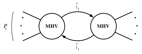
Figure 1: A generic MHV diagram contributing to the one-loop graviton MHV amplitude. The hatted loop momenta are defined below in (2.5).

The usual CSW off-shell prescription for calculating tree-level [3] and one-loop [29] amplitudes from MHV diagrams in Yang-Mills consists in decomposing any internal (off-shell) momentum $L$ as in (2.1), and using the holomorphic spinor $l_{\alpha}$ associated to the null momentum $l_{\alpha{\dot{\alpha}}}:=l_{\alpha}\widetilde{l}_{{\dot{\alpha}}}$ in the expression of the MHV vertices. In Yang-Mills, this prescription has been shown to work for a variety of cases at tree- [4, 5, 6, 7] and one-loop level [29, 36, 37, 38, 33, 44]. Moreover, Mansfield showed in [8] that it arises naturally in the framework of the lightcone quantisation of Yang-Mills theory, from which MHV rules are obtained via a particular change of variables in the functional integral.

Using $l_{1}$ and $l_{2}$ in the expressions of the vertices in place of the loop momenta $L_{1}$ and $L_{2}$ has the consequence of effectively “breaking” momentum conservation at each vertex – the momenta which are inserted in the expression of each MHV vertex do not sum to zero, as $l_{2}-l_{1}+P_{L}=z\eta\neq 0$. Interestingly, for tree-level Yang-Mills it was shown in [28] that momentum conservation can formally be reinstated by appropriately shifting the anti-holomorphic spinors of the momenta of the external negative-helicity particles. These shifts do not affect the Parke-Taylor expressions of the MHV vertices, as these only contain holomorphic spinors – they are invisible.

The situation in gravity is quite different. The infinite sequence of MHV amplitudes of gravitons was found by Berends, Giele and Kuijf in [53] and is given by an expression which contains both holomorphic and anti-holomorphic spinors (for a number of external gravitons larger than three). The new formula for the $n$-point graviton scattering amplitude found in [14] also contains holomorphic as well as anti-holomorphic spinors. Thus, it appears necessary to introduce a prescription for an off-shell continuation of anti-holomorphic spinors $\widetilde{l}_{{\dot{\alpha}}}$ related to the loop momenta. We look for this prescription in a way which allows us to solve a potential ambiguity which we now discuss.

We begin by observing that, a priori, several expressions for the same tree-level gravity MHV amplitude can be presented. For example, different realisations of the KLT relations [56] may be used, or different forms of the BCF recursion relations (two of which where considered in [14] and [15]). Upon making use of spinor identities and, crucially, of momentum conservation, one would discover that these different-looking expressions for the amplitudes are actually identical. However, without momentum conservation in place, these expressions are no longer equal. We conclude that if we do not maintain momentum conservation at each MHV vertex, we would face an ambiguity in selecting a specific form for the graviton MHV vertex – the expressions obtained by simply using the spinors $l_{i\alpha}$ and $\widetilde{l}_{i{\dot{\alpha}}}$ obtained from the null vectors $l_{i}=L_{i}-z_{i}\eta$, $i=1,2$ as in the Yang-Mills case, would in fact be different. Not surprisingly, the difference between any such two expressions amounts to $\eta$-dependent terms; stated differently, the expressions for the amplitudes naïvely continued off-shell would present us with spurious $\eta$-dependence. This ambiguity does not arise in the Yang-Mills case, where there is a preferred, holomorphic expression for the MHV amplitude of gluons, given by the Parke-Taylor formula.

We propose to resolve the ambiguity arising in the gravity case by resorting to certain shifts in the loop momenta, to be determined shortly, which have the effect of reinstating momentum conservation, in a way possibly reminiscent of the tree-level gravity MHV rules of [26]. As we shall see, these shifts determine a specific prescription for the off-shell continuation of the spinors associated to the loop legs.

Specifically, our procedure consists in interpreting the term $-z\eta$ in (2.2) as generated by a shift on the anti-holomorphic spinors of the loop momenta in the off-shell continuation of the MHV amplitudes. Absorbing this extra term into the definition of shifted momenta $\hat{l}_{1}$ and $\hat{l}_{2}$ allows us to preserve momentum conservation at each vertex also off shell. Indeed, we now write momentum conservation as

$$P_{L}+\hat{l}_{2}-\hat{l}_{1}\ =\ 0\ .$$ (2.4)

The hatted loop momenta are defined by a shift in the anti-holomorphic spinors,

$$\hat{l}_{1\alpha{\dot{\alpha}}}\ =\ l_{1\alpha}\hat{\widetilde{l}}_{1{\dot{\alpha}}}\ ,\quad\hat{l}_{2\alpha{\dot{\alpha}}}\ =\ l_{2\alpha}\hat{\widetilde{l}}_{2{\dot{\alpha}}}\ .$$ (2.5)

We find that the form of the shifts is natural and unique. Solving for the anti-holomorphic spinors $\hat{\widetilde{l}}_{1}$ and $\hat{\widetilde{l}}_{2}$, one gets

$$\hat{\widetilde{l}}_{1}\ =\ \widetilde{l}_{1}-z\,\frac{\langle l_{2}\eta\rangle}{\langle l_{1}l_{2}\rangle}\,\widetilde{\eta}\ ,$$

$$\hat{\widetilde{l}}_{2}\ =\ \widetilde{l}_{2}-z\,\frac{\langle l_{1}\eta\rangle}{\langle l_{1}l_{2}\rangle}\,\widetilde{\eta}\ .$$ (2.6)

It is easy to check that the contribution of the shifts is

$$l_{2\alpha}\delta\widetilde{l}_{2{\dot{\alpha}}}-l_{1\alpha}\delta\widetilde{l}_{1{\dot{\alpha}}}\ =\ -z\eta_{\alpha}\widetilde{\eta}_{{\dot{\alpha}}}\ ,$$ (2.7)

where we have used the Schouten identity $(\langle l_{1}\eta\rangle\,l_{2\alpha}-\langle l_{2}\eta\rangle\,l_{1\alpha})/\langle l_{1}l_{2}\rangle=\eta_{\alpha}$.

Our prescription (2) will then consist in replacing all the anti-holomorphic spinor variables associated to loop momenta with corresponding shifted spinors. For example, the spinor bracket $[l_{2}l_{1}]$ becomes

$$[\hat{l}_{2}\hat{l}_{1}]\ =\ [l_{2}l_{1}]-2z\,\frac{P_{L}\cdot\eta}{\langle l_{1}l_{2}\rangle}\ .$$ (2.8)

Notice also that

$$s_{\hat{l}_{1}-\hat{l}_{2}}\ :=\ (\hat{l}_{2}-\hat{l}_{1})^{2}=-\langle l_{1}l_{2}\rangle[\hat{l}_{2}\hat{l}_{1}]\ =\ P_{L}^{2}\ .$$ (2.9)

A few comments are now in order.

1. In [28], a derivation of tree-level MHV rules in Yang-Mills was discussed which makes use of shifts in the momenta of external legs. This approach was used in [26] where a long sought-after derivation of tree-level gravity MHV rules was presented. We differ from the approach of [28] and [26] in that we shift the momenta of the (off-shell) loop legs rather than the external momenta. It would clearly be interesting to find a first principle derivation of the shifts (2), perhaps from an action-based approach, along the lines of [8], as well as to relate our shifts to those employed at tree level in [26].

2. Our procedure of shifting the loop momenta in order to preserve momentum conservation off shell can also be applied to MHV diagrams in Yang-Mills. Indeed, using the Parke-Taylor expression for the MHV vertices would result in these shifts being invisible. We would like to point out that, in principle, one could use different expressions even for an MHV gluon scattering amplitude, possibly containing anti-holomorphic spinors. Had one chosen this second (unnecessarily complicated) path, our prescription (2) for shifts in anti-holomorphic spinors would guarantee that the non-holomorphic form of the vertex would always boil down to the Parke-Taylor form. Clearly, having to deal with holomorphic vertices, as in Yang-Mills, is a great simplification. The importance of holomorphicity of the MHV amplitudes is further appreciated in Mansfield’s derivation [8] of tree-level MHV rules in Yang-Mills.

In the next section we will test the ideas discussed earlier in a one-loop calculation in ${\cal N}=8$ supergravity, specifically that of a four-point MHV scattering amplitude of gravitons. We will then consider applications to amplitudes with arbitrary number of external particles.

3 Four-point MHV amplitude at one loop with MHV diagrams

In this section we will rederive the known expression for the four-point MHV scattering amplitude of gravitons ${\cal M}(1^{-}2^{-}3^{+}4^{+})$ using MHV rules. As in the Yang-Mills case, we will have to sum over all possible MHV diagrams, i.e. diagrams such that all the vertices have the MHV helicity configuration. Moreover, we will also sum over all possible internal helicity assignments, and over the particle species which can run in the loop. Specifically, we will focus on ${\cal N}=8$ supergravity, where all the one-loop amplitudes are believed to be expressible as sums of box functions only [19, 20, 18]. In this case, the result of [47, 48] is

$${\cal M}_{\rm 1-loop}^{{\cal N}=8}\ =\ {\cal M}^{\rm tree}\left[u\,F(1234)+t\,F(1243)+s\,F(1324)\right]\ ,$$ (3.1)

where ${\cal M}^{\rm tree}$ is the four-point MHV amplitude, and $F(ijkl)$ are zero-mass box functions with external, cyclically ordered null momenta $i$, $j$, $k$ and $l$. The kinematical invariants $s$, $t$, $u$ are defined as $s:=(k_{1}+k_{2})^{2}$, $t:=(k_{2}+k_{3})^{2}$, $u:=(k_{1}+k_{3})^{2}=-s-t$. We will see in our MHV diagrams approach that each box function appearing in (3.1) will emerge by summing over appropriate dispersion integrals of two-particle phase space integrals, similarly to the Yang-Mills case [29]. The result we will find is in complete agreement with the known expression found in [47, 48].

3.1 MHV diagrams in the $s$-, $t$-, and $u$-channels

We start by computing the MHV diagram in Figure 2. This diagram has a nontrivial $s$-channel cut, hence we will refer to it as to the “$s$-channel MHV diagram”. Its expression is given by

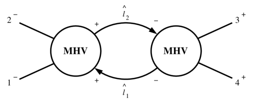
Figure 2: The $s$-channel MHV diagram.

$${\cal M}_{s}\ =\ \int\!d\mu_{k_{1}+k_{2}}\ {\cal M}(1^{-}2^{-}\hat{l}_{2}^{+}-\hat{l}_{1}^{+})\ {\cal M}(\hat{l}_{1}^{-}-\hat{l}_{2}^{-}3^{+}4^{+})\ .$$ (3.2)

The integration measure $d\mu_{P_{L}}$ is [29]

$$d\mu_{P_{L}}\ =\ \frac{d^{4}L_{1}}{L_{1}^{2}+i\varepsilon}\frac{d^{4}L_{2}}{L_{2}^{2}+i\varepsilon}\ \delta^{(4)}(L_{2}-L_{1}+P_{L})\ ,$$ (3.3)

where, for the specific case of (3.2), we have $P_{L}=k_{1}+k_{2}$. Notice the hats in (3.2), which stand for the shifts defined in (2). These shifts are such to preserve momentum conservation off shell, hence we can use any of the (now equivalent) forms of MHV amplitudes of gravitons as off-shell vertices. We choose the expression for the four-graviton MHV amplitude obtained by applying the KLT relation (C.3), thus getting

$${\cal M}(1^{-}2^{-}\hat{l}_{2}^{+}-\hat{l}_{1}^{+}) = -is_{12}\,{\cal A}(1^{-}2^{-}l_{2}^{+}-l_{1}^{+})\,{\cal A}(1^{-}2^{-}-l_{1}^{+}l_{2}^{+})\ ,$$ (3.4)

$${\cal M}(\hat{l}_{1}^{-}-\hat{l}_{2}^{-}3^{+}4^{+}) = -is_{\hat{l}_{1}-\hat{l}_{2}}\,{\cal A}(l_{1}^{-}-l_{2}^{-}3^{+}4^{+})\,{\cal A}(l_{1}^{-}-l_{2}^{-}4^{+}3^{+})\ ,$$ (3.6)

where ${\cal A}$’s are Yang-Mills amplitudes. We need not shift the $l$’s appearing inside the gauge theory amplitudes, as these are holomorphic in the spinor variables.

Using the Parke-Taylor formula for the MHV amplitudes and the result (2.9), the $s$-channel MHV diagram gives

$${\cal M}_{s}\ =\ -\frac{\langle 12\rangle^{8}}{\langle 12\rangle^{2}\langle 34\rangle^{2}}\,s^{2}\,\int\!d\mu_{k_{1}+k_{2}}\ \,\frac{\langle l_{1}l_{2}\rangle^{4}}{\langle 1l_{1}\rangle\langle 2l_{1}\rangle\langle 3l_{1}\rangle\langle 4l_{1}\rangle\langle 1l_{2}\rangle\langle 2l_{2}\rangle\langle 3l_{2}\rangle\langle 4l_{2}\rangle}\ .$$ (3.7)

Figure 3: The $t$-channel MHV diagram. The $u$-channel diagram is obtained by exchanging gravitons $1^{-}$ and $2^{-}$.

Two more MHV diagrams with a non-null two-particle cut contribute to the one-loop four-graviton amplitude, see Figure 3. Since these have a nontrivial $t$-channel, or $u$-channel two-particle cut, we will call them $t$-channel, and $u$-channel MHV diagram, respectively. For these diagrams, all particles in the ${\cal N}=8$ supergravity multiplet can run in the loop, and moreover we will have to sum over the two possible internal helicity assignments. Using supersymmetric Ward identities [55, 54] it is possible to write this sum over contributions from all particles running in the loop as the contribution arising from a scalar loop times a purely holomorphic quantity $\rho_{{\cal N}=8}$ [48], where

$$\rho_{{\cal N}=8}\ :=\ \frac{\langle 12\rangle^{8}\langle l_{1}l_{2}\rangle^{8}}{(\langle 1l_{2}\rangle\langle 2l_{1}\rangle\langle 1l_{1}\rangle\langle 2l_{2}\rangle)^{4}}\ .$$ (3.8)

It is then easy to check that the results in the $t$- and $u$-channels are exactly the same as the $s$-channel, with the appropriate relabeling of the external legs (apart from the overall factor $\langle 12\rangle^{8}$). For example, in the $t$-channel we find

$${\cal M}_{t}\ =\ -\frac{\langle 12\rangle^{8}}{\langle 23\rangle^{2}\langle 41\rangle^{2}}\,t^{2}\,\int\!d\mu_{k_{2}+k_{3}}\ \,\frac{\langle l_{1}l_{2}\rangle^{4}}{\langle 1l_{1}\rangle\langle 2l_{1}\rangle\langle 3l_{1}\rangle\langle 4l_{1}\rangle\langle 1l_{2}\rangle\langle 2l_{2}\rangle\langle 3l_{2}\rangle\langle 4l_{2}\rangle}\ .$$ (3.9)

Making use of momentum conservation, it is immediate to see that the prefactors of (3.7) and (3.9) are identical, $s^{2}/(\langle 12\rangle\langle 34\rangle)^{2}=t^{2}/(\langle 23\rangle\langle 41\rangle)^{2}$.

We will discuss the specific evaluation of the $s$-channel MHV diagram (3.7) and the $t$- and $u$-channel diagrams in section 3.3. Before doing so, we would like to first write the expressions of the remaining MHV diagrams, which have a null two-particle cut.

3.2 Diagrams with null two-particle cut

In the unitarity-based approach of BDDK, diagrams with a null two-particle cut are of course irrelevant, as they do not have a discontinuity. However in the MHV diagram method we have to consider them [29, 37, 38]. As also observed in the calculation of the gauge theory amplitudes considered in those papers, we will see that these diagrams give rise to contributions proportional to dispersion integrals of (one-mass or zero-mass) boxes in a channel with null momentum. For generic choices of $\eta$ the contribution of these diagrams is non-vanishing, and important in order to achieve the cancellation of $\eta$-dependent terms. For specific, natural choices of $\eta$ [29], one can see that these diagrams actually vanish by themselves; see appendix A for a discussion of this point.

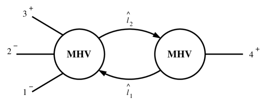
Figure 4: One of the MHV diagrams with a null two-particle cut.

To be specific, let us consider the diagram with particles 1, 2 and 3 on the left, and particle 4 on the right (see Figure 4). The remaining three diagrams (with particle 4 replaced by particles 1, 2, and 3, respectively) are obtained by relabeling the external particles and summing over the particles running in the loop, when required.

The action of the shifts (2) allows us to preserve momentum conservation off shell in the form

$$k_{1}+k_{2}+k_{3}+\hat{l}_{2}-\hat{l}_{1}\ =\ 0\ ,$$ (3.10)

on the left, and

$$k_{4}-\hat{l}_{2}+\hat{l}_{1}\ =\ 0\ ,$$ (3.11)

on the right. Equations (3.10) and (3.11) again imply that global momentum conservation $\sum_{i=1}^{4}k_{i}=0$ is also preserved.

The expression for the diagram in Figure 4 is given by

$${\cal M}_{k_{4}^{2}}\ =\ \int\!d\mu_{k_{4}}\ {\cal M}(1^{-}2^{-}3^{+}\hat{l}_{2}^{+}-\hat{l}_{1}^{+})\ {\cal M}(\hat{l}_{1}^{-}-\hat{l}_{2}^{-}4^{+})\ .$$ (3.12)

In order to obtain an expression for the five-point tree-level vertex entering (3.12), we apply the KLT relation (C.4), whereas for the three-point vertex we simply use (C.1). Thus, we get

$${\cal M}_{k_{4}^{2}}\ =\ \int\!d\mu_{k_{4}}\ \left[s_{12}s_{3\hat{l}_{2}}\,{\cal A}(1^{-}2^{-}3^{+}l_{2}^{+}-l_{1}^{+}){\cal A}(2^{-}1^{-}l_{2}^{+}3^{+}-l_{1}^{+})\right.$$

$$\left.\ \ \ +\,s_{13}s_{2\hat{l}_{2}}\,{\cal A}(1^{-}3^{+}2^{-}l_{2}^{+}-l_{1}^{+}){\cal A}(3^{+}1^{-}l_{2}^{+}2^{-}-l_{1}^{+})\right]\left[{\cal A}(l_{1}^{-}-l_{2}^{-}4^{+})\right]^{2}\ ,$$ (3.13)

where the vector $\hat{l}_{2}$ is shifted.

We can now rewrite (3.2) as

$${\cal M}_{k_{4}^{2}}\ = \ \frac{\langle 12\rangle^{8}}{\langle 12\rangle\langle 13\rangle\langle 32\rangle}\int\!d\mu_{k_{4}}\ \left[\langle 13\rangle[21]\langle 2l_{2}\rangle[\hat{l}_{2}3]-\langle 12\rangle[31]\langle 3l_{2}\rangle[\hat{l}_{2}2]\right]\cdot$$ (3.14)

$$\cdot \ \ \frac{\langle l_{1}l_{2}\rangle^{5}}{\langle 1l_{1}\rangle\langle 1l_{2}\rangle\langle 2l_{1}\rangle\langle 2l_{2}\rangle\langle 3l_{1}\rangle\langle 3l_{2}\rangle\langle 4l_{1}\rangle^{2}\langle 4l_{2}\rangle^{2}}\ \ .$$

Notice that apparently (3.14) contains unphysical double poles in $\langle 4l_{1}\rangle$ and $\langle 4l_{2}\rangle$, generated by the presence of the three-point vertex $\left[{\cal A}(l_{1}^{-}-l_{2}^{-}4^{+})\right]^{2}$ in (3.2). What we are going to show is that thanks to momentum conservation – now always preserved in terms of the shifted momenta – these double poles disappear. Furthermore, we will show that the integrand has exactly the same form as that in (3.7), obtained from diagrams with a two-particle cut.

We start by factorising out of the integrand (3.14) the quantity

$$Q\>=\ \frac{\langle l_{1}l_{2}\rangle^{4}}{\prod_{i=1}^{4}\langle il_{2}\rangle\ \prod_{j=1}^{4}\langle jl_{1}\rangle}\ .$$ (3.15)

We are then left with

$$\frac{\langle 12\rangle^{8}}{\langle 12\rangle\langle 13\rangle\langle 32\rangle}\,\left[\langle 13\rangle[21]\langle 2l_{2}\rangle[\hat{l}_{2}3]-\langle 12\rangle[31]\langle 3l_{2}\rangle[\hat{l}_{2}2]\right]\,\frac{\langle l_{1}l_{2}\rangle}{\langle 4l_{1}\rangle\langle 4l_{2}\rangle}\ .$$ (3.16)

By using momentum conservation (3.11) on the right hand side MHV vertex, we can rewrite (3.16) as

$$\frac{\langle 12\rangle^{8}}{\langle 12\rangle\langle 13\rangle\langle 32\rangle}\,\left[\langle 13\rangle[21][34]\frac{\langle 2l_{2}\rangle}{\langle 4l_{2}\rangle}-\langle 12\rangle[31][24]\frac{\langle 3l_{2}\rangle}{\langle 4l_{2}\rangle}\right]\ .$$ (3.17)

Using momentum conservation $\sum_{i=1}^{4}k_{i}=0$ in the form

$$\langle 3l_{2}\rangle[31]\ =\ -\langle 4l_{2}\rangle[41]-\langle 2l_{2}\rangle[21]\ ,$$ (3.18)

we get

$$\frac{\langle 12\rangle^{8}}{\langle 12\rangle\langle 13\rangle\langle 32\rangle}\,\left[\langle 12\rangle[24][41]+(\langle 13\rangle[34]+\langle 12\rangle[24])[21]\frac{\langle 2l_{2}\rangle}{\langle 4l_{2}\rangle}\right]\ =\ \frac{\langle 12\rangle^{8}}{\langle 12\rangle\langle 13\rangle\langle 32\rangle}\langle 12\rangle[24][41]\ .$$ (3.19)

The surprise is that the coefficient (3.19) is actually the negative of the prefactor which multiplies the integral in the expression (3.7) for the MHV diagrams corresponding to the $s$-channel. We can thus rewrite (3.14) as

$${\cal M}_{k_{4}^{2}}\ =\ \frac{\langle 12\rangle^{8}}{\langle 12\rangle^{2}\langle 34\rangle^{2}}\,s^{2}\,\int\!d\mu_{k_{4}}\ \,\frac{\langle l_{1}l_{2}\rangle^{4}}{\langle 1l_{1}\rangle\langle 2l_{1}\rangle\langle 3l_{1}\rangle\langle 4l_{1}\rangle\langle 1l_{2}\rangle\langle 2l_{2}\rangle\langle 3l_{2}\rangle\langle 4l_{2}\rangle}\ ,$$ (3.20)

which is the opposite of the right hand side of (3.7) – except for the integration measure $d\mu_{k_{4}^{2}}$ appearing in (3.20), which is different from that in (3.7) (as the momentum flowing in the cut is different). As we shall see in the next section, the relative minus sign found in (3.20) compared to (3.7) is precisely needed in order to reconstruct box functions from summing dispersive integrals (see (3.60)), one for each cut, as it was found in [29].

3.3 Explicit evaluation of the one-loop MHV diagrams

In the last sections we have encountered a peculiarity of the gravity calculation, namely the fact that the expression for the integrand of each MHV diagram contributing to the four-point graviton MHV amplitude turns out to be the same – compare, for example, (3.7), (3.9), (3.20), which correspond to the $s$-, $t$-, and $k_{4}^{2}$-channel MHV diagram, respectively. Therefore we will focus on the expression of a generic contribution of these MHV diagrams, for example from (3.7),

$${\cal M}\ =\ -\frac{\langle 12\rangle^{8}}{\langle 12\rangle^{2}\langle 34\rangle^{2}}\,s^{2}\,\int\!d\mu_{P_{L}}\ \,\frac{\langle l_{1}l_{2}\rangle^{4}}{\langle 1l_{1}\rangle\langle 2l_{1}\rangle\langle 3l_{1}\rangle\langle 4l_{1}\rangle\langle 1l_{2}\rangle\langle 2l_{2}\rangle\langle 3l_{2}\rangle\langle 4l_{2}\rangle}\ ,$$ (3.21)

and perform the relevant phase space and dispersion integrals.

In order to evaluate (3.21), we need to perform the PV reduction of the phase-space integral of the quantity $Q$ defined in (3.15). To carry out this reduction efficiently, we use the trick of performing certain auxiliary shifts, which allow us to decompose (3.15) in partial fractions. Each term produced in this way will then have a very simple PV reduction.

Firstly, we write $Q$ as

$$Q\ :=\langle l_{1}l_{2}\rangle^{4}\,\ X\,Y\,\ ,$$ (3.22)

where

$$X = \frac{1}{\prod_{i=1}^{4}\langle il_{2}\rangle}\ ,$$ (3.23)

$$Y = \frac{1}{\prod_{j=1}^{4}\langle jl_{1}\rangle}\ ,$$ (3.24)

and perform the following auxiliary shift

$$\hat{\lambda}_{l_{2}}\ =\ \lambda_{l_{2}}+\omega\lambda_{l_{1}}\ ,$$ (3.25)

on the quantity $X$ in (3.23) (we will later apply the same procedure on $Y$). We call $\hat{X}$ the corresponding shifted quantity,

$$\hat{X}\ =\ \frac{1}{\prod_{i=1}^{4}(\langle il_{2}\rangle+\omega\langle il_{1}\rangle)}\ .$$ (3.26)

Next, we decompose $\hat{X}$ in partial fractions, and finally set $\omega=0$. After using the Schouten identity, we find that $X$ can be recast as

$$X\ =\ \frac{1}{\langle l_{1}l_{2}\rangle^{3}}\sum_{i=1}^{4}\,\frac{\langle il_{1}\rangle^{3}}{\prod_{m\neq i}\langle im\rangle}\,\frac{1}{\langle il_{2}\rangle}\ .$$ (3.27)

One can proceed in a similar way for $Y$ defined in (3.24), and, in conclusion, (3.15) is re-expressed as

$$Q\ =\ \sum_{i,j=1}^{4}\,\frac{1}{\prod_{m\neq i}\langle im\rangle}\,\frac{1}{\prod_{l\neq j}\langle jl\rangle}\,\frac{1}{\langle l_{1}l_{2}\rangle^{2}}\,\frac{\langle il_{1}\rangle^{3}\,\langle jl_{2}\rangle^{3}}{\langle il_{2}\rangle\,\langle jl_{1}\rangle}\ .$$ (3.28)

We now set

$$Q\ =\ \sum_{i,j=1}^{4}\,\frac{1}{\prod_{m\neq i}\langle im\rangle}\,\frac{1}{\prod_{l\neq j}\langle jl\rangle}\ K\ ,$$ (3.29)

where

$$K\ :=\ \frac{1}{\langle l_{1}l_{2}\rangle^{2}}\,\frac{\langle il_{1}\rangle^{3}\,\langle jl_{2}\rangle^{3}}{\langle il_{2}\rangle\,\langle jl_{1}\rangle}\ ,$$ (3.30)

and substitute the Schouten identity for the factor $(\langle il_{1}\rangle\langle jl_{2}\rangle)^{2}$ in $K$. By multiplying for appropriate anti-holomorphic inner products (of unshifted spinors), we are able to reduce $K$ to the sum of three terms as follows:

$$K\ =\ \frac{\langle i|\,l_{2}P_{L;z}\,|i\rangle\langle j|\,l_{2}P_{L;z}\,|j\rangle}{(P_{L;z}^{2})^{2}}+2\langle ij\rangle\frac{\langle j|\,l_{2}P_{L;z}\,|i\rangle}{P_{L;z}^{2}}+\langle ij\rangle^{2}R(ji)\ ,$$ (3.31)

where

$$P_{L;z}\ :=\ P_{L}-z\eta\ ,$$ (3.32)

and $z$ is defined in (2.3). The first term in (3.31) gives two-tensor bubble integrals, the second linear bubbles, and the third term generates the usual $R$-function, familiar from the Yang-Mills case. This is defined by

$$R(ji)\ =\ \frac{\langle jl_{2}\rangle\langle il_{1}\rangle}{\langle jl_{1}\rangle\langle il_{2}\rangle}\ .$$ (3.33)

We can then decompose the $R$ function as

$$R(ji)\ = \ \frac{2\left[(l_{1}j)(l_{2}i)+(l_{1}i)(l_{2}j)-(l_{1}l_{2})(ij)\right]}{(l_{1}-j)^{2}(l_{2}+j)^{2}}\$$

$$= \ -1+\frac{1}{2}\left[\frac{P_{L;z}i}{l_{2}i}-\frac{P_{L;z}j}{l_{1}j}\right]+\frac{2(iP_{L;z})(jP_{L;z})-P_{L;z}^{2}(ij)}{4(l_{2}i)(l_{1}j)}\ .$$ (3.34)

The phase-space integral of the first term on the right hand side of (3.3) corresponds to a scalar bubble, whereas the second and the third one correspond to triangles; finally, the phase-space integral of the last term in (3.3) gives rise to a box function. The last term is usually called $R^{\rm eff}(ji)$,

$$R^{\rm eff}(ji)\ :=\ \frac{N(P_{L;z})}{(l_{1}-j)^{2}\,(l_{2}+i)^{2}}\ ,$$ (3.35)

where

$$N(P_{L;z})\ :=\ -2(iP_{L;z})\,(jP_{L;z})+P_{L;z}^{2}(ij)\ .$$ (3.36)

We now show the cancellation of bubbles and triangles, which leaves us just with box functions.

To start with, we pick all contributions to (the phase-space integral of) (3.29) corresponding to scalar, linear and two-tensor bubbles, which we identify using (3.31). These are given by

$$Q_{\rm bubbles}\ =\ \sum_{i,j=1}^{4}\,\frac{1}{\prod_{m\neq i}\langle im\rangle}\,\frac{1}{\prod_{l\neq j}\langle jl\rangle}\ \left[\frac{\langle i|\,l_{2}P_{L;z}\,|i\rangle\langle j|\,l_{2}P_{L;z}\,|j\rangle}{(P_{L;z}^{2})^{2}}+2\langle ij\rangle\frac{\langle j|\,l_{2}P_{L;z}\,|i\rangle}{P_{L;z}^{2}}-\langle ij\rangle^{2}\right]\ .$$ (3.37)

Explicitly, the phase-space integrals of linear and two-tensor bubbles are given by

$$I^{\mu}\ =\ \int\!d\textrm{LIPS}(l_{2},-l_{1};P_{L;z})\ l_{2}^{\mu}\ =\ -\frac{1}{2}\,P_{L;z}^{\mu}\ ,$$ (3.38)

and

$$I^{\mu\nu}\ =\ \int\!\ d\textrm{LIPS}(l_{2},-l_{1};P_{L,z})\ l_{2}^{\mu}\,l_{2}^{\nu}\ =\ \frac{1}{3}\left[P_{L;z}^{\mu}P_{L;z}^{\nu}-\frac{1}{4}\eta^{\mu\nu}P_{L;z}^{2}\right]\ .$$ (3.39)

Thus, we find that the bubble contributions arising from (3.37) give a result proportional to

$$C = \sum_{i,j=1}^{4}\,\frac{\langle ij\rangle^{2}}{\prod_{m\neq i}\langle im\rangle\prod_{l\neq j}\langle jl\rangle}\,\ .$$ (3.40)

Using the Schouten identity, it is immediate to show that $C=0$. We remark that the previous expression vanishes also for a fixed value of $i$.

We now move on to consider the triangle contributions. From (3.29) and (3.3), we get

$$Q_{\rm triangles}\ =\ \sum_{i,j=1}^{4}\,\frac{1}{\prod_{m\neq i}\langle im\rangle}\,\frac{1}{\prod_{l\neq j}\langle jl\rangle}\ \frac{\langle ij\rangle^{2}}{2}\left[\frac{P_{L;z}i}{l_{2}i}-\frac{P_{L;z}j}{l_{1}j}\right]\ .$$ (3.41)

We observe that the combination

$$\int\!d{\rm LIPS}\ \left[\frac{P_{L;z}j}{l_{1}j}-\frac{P_{L;z}i}{l_{2}i}\right]\ =\ -\frac{4\pi\lambda}{\epsilon}\ ,$$ (3.42)

is independent of $i$ and $j$ [37], hence we can bring the corresponding term in (3.41) outside the summation, obtaining again a contribution proportional to the coefficient (3.40), which vanishes; this proves the cancellation of triangles. We conclude that each one-loop MHV diagram is written just in terms of box functions, and is explicitly given by

$${\cal M}\ =\ -\frac{\langle 12\rangle^{8}}{\langle 12\rangle^{2}\langle 34\rangle^{2}}\,s^{2}\,\int\!d\mu_{P_{L}}\,\,\sum_{i\neq j}\,\frac{\langle ij\rangle^{2}}{\prod_{m\neq i}\langle im\rangle\,\prod_{l\neq j}\langle jl\rangle}\frac{N(P_{L;z})}{(l_{1}-j)^{2}\,(l_{2}+i)^{2}}\ .$$ (3.43)

We remind that $P_{L}$ is the sum of the (outgoing) momenta in the left hand side MHV vertex. To get the full amplitude at one loop we will then have to sum over all possible MHV diagrams.

The next task consists in performing the loop integration. To do this, we follow steps similar to those discussed in [29], namely:

1. We rewrite the integration measure as the product of a Lorentz-invariant phase space measure and an integration over the $z$-variables (one for each loop momentum) introduced by the off-shell continuation,

$$d\mu_{P_{L}}\ :=\ \frac{d^{4}L_{1}}{L_{1}^{2}}\frac{d^{4}L_{2}}{L_{2}^{2}}\ \delta^{(4)}(L_{2}-L_{1}+P_{L})\ =\ \frac{dz_{1}}{z_{1}}\frac{dz_{2}}{z_{2}}\,d{\rm LIPS}(l_{2},-l_{1};P_{L;z})\ .$$ (3.44)

2. We change variables from $(z_{1},z_{2})$ to $(z,z^{\prime})$, where $z^{\prime}:=z_{1}+z_{2}$ and $z$ is defined in (2.3), and perform a trivial contour integration over $z^{\prime}$.

3. We use dimensional regularisation on the phase-space integral of the boxes,

$${\cal P}\ =\ \int\!d^{D}{\rm{LIPS}}(l_{2},-l_{1};P_{L})\ \frac{N(P_{L})}{(l_{1}-j)^{2}\,(l_{2}+i)^{2}}\ .$$ (3.45)

This evaluates to all orders in $\epsilon$ to

$${\cal P}\ =\ \frac{\pi^{\frac{3}{2}-\epsilon}}{\Gamma(\frac{1}{2}-\epsilon)}\,\frac{1}{\epsilon}\,\left|\frac{P_{L}^{2}}{4}\right|^{-\epsilon}\,{}_{2}F_{1}(1,-\epsilon,1-\epsilon,aP_{L}^{2})\ ,$$ (3.46)

where

$$a\ :=\ \frac{P^{2}+Q^{2}-s-t}{P^{2}Q^{2}-st}\ .$$ (3.47)

The phase space integral in (3.46) is computing a particular discontinuity of the box diagram represented in in Figure 5, with $p=i$ and $q=j$, where the cut momentum is $P_{L}$.

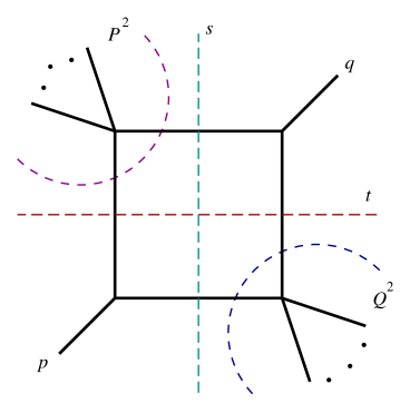
Figure 5: A generic two-mass easy box function. $p$ and $q$ are the massless legs, $P$ and $Q$ the massive ones, and $s:=(P+p)^{2}$, $t:=(P+q)^{2}$.

4. We perform the final $z$-integral by defining the new variable

$$s^{\prime}\ :=\ P_{L;z}^{2}\ =\ P_{L}^{2}-2zP_{L}\cdot\eta\ .$$ (3.48)

One notices that [29]

$$\frac{dz}{z}\ :=\ \frac{ds^{\prime}}{s^{\prime}-P_{L}^{2}}\ ,$$ (3.49)

hence the $z$-integral leads to a dispersion integral in the $P_{L}^{2}$-channel. At this point we select a specific value for $\eta$, namely we choose it to be equal to the momentum of particles $j$ or $i$. Specifically, performing the phase-space integration and the dispersive integral for a box in the $P_{L}^{2}$-channel, we get

$$\int\!d\mu_{P_{L}}\,\frac{N(P_{L;z})}{(l_{1}-j)^{2}\,(l_{2}+i)^{2}} = -\frac{c_{\Gamma}}{\epsilon^{2}}\,(-P_{L}^{2})^{-\epsilon}\,{}_{2}F_{1}(1,-\epsilon,1-\epsilon,aP_{L}^{2})$$ (3.50)

$$:= F_{P_{L}^{2}}(p,P,q,Q)\ ,$$ (3.51)

where

$$c_{\Gamma}\ :=\ {\Gamma(1+\epsilon)\Gamma^{2}(1-\epsilon)\over(4\pi)^{2-\epsilon}\Gamma(1-2\epsilon)}\ .$$ (3.52)

The subscript $P_{L}$ refers to the dispersive channel in which (3.50) is evaluated; the arguments of $F_{P_{L}^{2}}$ correspond to the ordering of the external legs of the box function.

We can rewrite (3.43) as

$${\cal M}\ =\ -2\,\frac{\langle 12\rangle^{8}}{\langle 12\rangle^{2}\langle 34\rangle^{2}}\,s^{2}\,\int\!d\mu_{P_{L}}\,\,\sum_{i<j}\,\frac{\langle ij\rangle^{2}}{\prod_{m\neq i}\langle im\rangle\,\prod_{l\neq j}\langle jl\rangle}\frac{N(P_{L;z})}{(l_{1}-j)^{2}\,(l_{2}+i)^{2}}\ ,$$ (3.53)

or, in terms of the $R^{\rm eff}$ functions introduced in (3.35),

$${\cal M} = -2\,\frac{\langle 12\rangle^{8}}{\langle 12\rangle^{2}\langle 34\rangle^{2}}\,s^{2}\,\int\!d\mu_{P_{L}}\,\,\bigg{[}\frac{R^{\rm eff}(13)+R^{\rm eff}(24)}{\langle 12\rangle\langle 14\rangle\langle 32\rangle\langle 34\rangle}+\frac{R^{\rm eff}(23)+R^{\rm eff}(14)}{\langle 12\rangle\langle 13\rangle\langle 42\rangle\langle 43\rangle}$$ (3.55)

$$\hskip 102.43008pt+\ \frac{R^{\rm eff}(12)+R^{\rm eff}(34)}{\langle 13\rangle\langle 14\rangle\langle 23\rangle\langle 24\rangle}\bigg{]}\ .$$

For the sake of definiteness, we now specify the PV reduction we have performed to the $s$-channel MHV diagram ($P_{L}\ =\ k_{1}+k_{2}$), and analyse in detail the contributions to the different box functions. In this case, the first two $R$-functions contribute to the box $F(1234)$, and the second two to the box $F(1243)$. Specifically, from these terms we obtain

$${\cal M}^{\rm tree}\left[u\,F_{s}(1234)\,+\,t\,F_{s}(1243)\right]\ ,$$ (3.56)

where the subscript indicates the channel in which the dispersion integral is performed ($s:=s_{12}$), and

$${\cal M}^{\rm tree}\ :=\ \frac{\langle 12\rangle^{7}\,[12]}{\langle 13\rangle\langle 14\rangle\langle 23\rangle\langle 24\rangle\langle 34\rangle^{2}}\$$ (3.57)

is the tree-level four-graviton MHV scattering amplitude.

The last two terms in (3.55) give a contribution to particular box diagrams where one of the external legs happens to have a vanishing momentum.

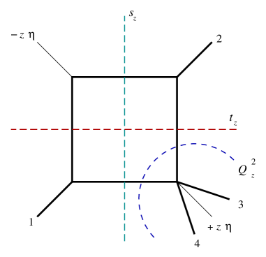
Figure 6: Cut-box function, where – before dispersive integration – one of the external legs has a momentum proportional to $z\eta$.

In principle, these boxes are reconstructed, as all the others, by summing over dispersion integrals in their cuts (note that in this case there is one cut missing, corresponding to the $\eta^{2}$-channel). However, one can see that these box diagrams give a vanishing contribution already at the level of phase space integrals, when $\eta$ is chosen, for each box, in exactly the same way as in the Yang-Mills calculation of [29]. For example, consider the box diagram in Figure 6, for which these natural choices are $\eta=k_{1}$ or $\eta=k_{2}$. Prior to the dispersive integration, this box has three nontrivial cuts: $s_{z}=(k_{1}-z\eta)^{2}$, $t_{z}=(k_{2}-z\eta)^{2}$, and $Q_{z}^{2}=(k_{3}+k_{4}+z\eta)^{2}$. Using (3.46) to perform the phase space integrals, one encounters two distinct cases: either the quantity $aP_{L;z}^{2}$ is finite but $P_{L;z}^{2}\to 0$ ($P_{L;z}$ is the momentum flowing in the cut); or $aP_{L;z}^{2}\to\infty$. It is then easy to see that in both cases the corresponding contribution vanishes. The conclusion is that such boxes can be discarded altogether. For the same reason these diagrams were discarded in the Yang-Mills case.

Next, we consider the $t$-channel MHV diagram. In this case the second term in (3.55) gives contribution to vanishing boxes like that depicted in Figure 6, the first and last terms instead give the contribution:

$${\cal M}^{\rm tree}\Big{[}u\,F_{t}(1234)\,+\,s\,F_{t}(1324)\Big{]}\ .$$ (3.58)

Similarly, for the $u$-channel we obtain:

$${\cal M}^{\rm tree}\Big{[}s\,F_{u}(1324)\,+\,t\,F_{u}(1243)\Big{]}\ .$$ (3.59)

Again the subscript indicates the channel in which the dispersion integral is performed ($t:=s_{23}$ and $u:=s_{13}$).

As in the Yang-Mills case, we have to sum over all possible MHV diagrams. In particular, we will also have to include the $k_{1}^{2}$-, $k_{2}^{2}$-, $k_{3}^{2}$- and $k_{4}^{2}$-channel MHV diagrams. In section 3.2 we have seen that, prior to the phase space and dispersive integration, these diagrams produce expressions identical up to a sign to those in the $s$-, $t$-, and $u$-channels. Hence they will give rise to dispersion integrals of the same cut-boxes found in those channels, this time in their $P^{2}$- and $Q^{2}$-cuts. They appear with the same coefficient, but opposite sign. We can thus collect dispersive integrals in different channels of the same box function, which appear with the same coefficient, and use the result proven in [29]

$$F\ =\ F_{s}+F_{t}-F_{P^{2}}-F_{Q^{2}}\ ,$$ (3.60)

in order to reconstruct each box function from the four dispersion integrals in its $s$-, $t$-, $P^{2}$- and $Q^{2}$- channels. For completeness, we quote from [33] the all orders in $\epsilon$ expression for a generic two-mass easy box function,

$$F=-{c_{\Gamma}\over\epsilon^{2}}\left[\Big{(}{-s\over\mu^{2}}\Big{)}^{-\epsilon}\,\mbox{}_{2}F_{1}\left(1,-\epsilon,1-\epsilon,as\right)\,+\,\Big{(}{-t\over\mu^{2}}\Big{)}^{-\epsilon}\mbox{}_{2}F_{1}\left(1,-\epsilon,1-\epsilon,at\right)\right.$$

(3.61)

$$\!-\,\left.\Big{(}{-P^{2}\over\mu^{2}}\Big{)}^{-\epsilon}\,\mbox{}_{2}F_{1}\left(1,-\epsilon,1-\epsilon,aP^{2}\right)\,-\,\Big{(}{-Q^{2}\over\mu^{2}}\Big{)}^{-\epsilon}\,\mbox{}_{2}F_{1}\left(1,-\epsilon,1-\epsilon,aQ^{2}\right)\right]\,,$$ (3.62)

where $c_{\Gamma}$ is defined in (3.52).

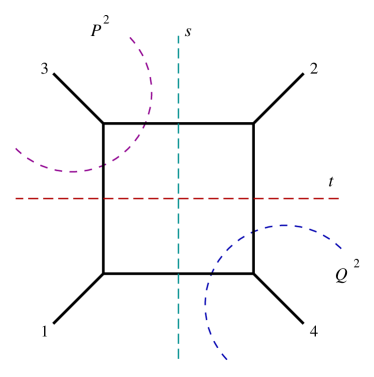
Figure 7: The box function $F(1324)$, appearing in the four-point amplitude (3.64).

As an example, we discuss in more detail how the box $F(1324)$ (depicted in Figure 7) is reconstructed. Due to the degeneracy related to the particular case of four particles, both the $R$-functions $R(12)$ and $R(34)$ give contribution to this box (see the third term in the result (3.55)). Let us focus on the contribution from the function $R(12)$, corresponding to the box in Figure 7. This box function gets contributions from MHV diagrams in the channels $u=s_{13}$, $t=s_{32}$, $k_{3}^{2}$ and $k_{4}^{2}$. They all appear with the same coefficient, given by the third term in (3.55), the last two contributions having opposite sign, as shown (we note that for all the others diagrams this term in the result gives contribution to vanishing boxes, as the one in Figure 6). These four contributions to the box $F(1324)$ correspond to its cuts in the $s=s_{13}$-, $t=s_{32}$-, $P^{2}=k_{3}^{2}$- and $Q^{2}\!=\!k_{4}^{2}$-channels. By summing over these four dispersion integrals using (3.60), we immediately reconstruct the box function $F(1324)$, which appear with a coefficient

$${\cal M}^{\rm tree}(1^{-}2^{-}3^{+}4^{+})\,s\,F(1324)\ .$$ (3.63)

This procedure can be applied in an identical fashion to reconstruct the other box functions. Summing over the contributions from all the different channels, and using (3.60) to reconstruct all the box functions we arrive at the final result

$${\cal M}^{1-{\rm loop}}(1^{-}2^{-}3^{+}4^{+})\ =\ {\cal M}^{\rm tree}(1^{-}2^{-}3^{+}4^{+})\,\left[\,u\,F(1234)\,+\,t\,F(1243)\,+\,s\,F(1324)\,\right]\ .$$ (3.64)

This is in complete agreement with the result of [48] found using the unitarity-based method.

4 Five-point amplitudes

We would like to discuss how the previous calculations can be extended to the case of scattering amplitudes with more than four particles. To be specific, we consider the five-point MHV amplitude of gravitons ${\cal M}(1^{-}2^{-}3^{+}4^{+}5^{+})$. Clearly, increasing the number of external particles leads to an increase in the algebraic complexity of the problem. However, the same basic procedure discussed in the four-particle case can be applied; in particular, we observe that the shifts (2) can be used for any number of external particles. This set of shifts allows one to use any on-shell technique of reduction of the integrand. In appendix B we propose a reduction technique alternative to that used in this and in section 3, which can easily be applied to the case of an arbitrary number of external particles.

We now consider the MHV diagrams contributing to the five-particle MHV amplitude. We start by computing the MHV diagrams which have a non-null two-particle cut. Firstly, consider the diagram pictured in Figure 8. Its expression is given by

Figure 8: MHV diagram contributing to the five-point MHV amplitude discussed in the text.

$${\cal M}^{1-{\rm loop}}_{(123)(45)}\ =\ \int\!d\mu_{P_{123}}\ {\cal M}(1^{-}2^{-}3^{+}l_{2}^{+}-l_{1}^{+})\ {\cal M}(l_{1}^{-}-l_{2}^{-}4^{+}5^{+})\ ,$$ (4.1)

where $d\mu_{P_{L}}$ is given by (3.3) and $P_{123}:=k_{1}+k_{2}+k_{3}$. We make use of the off-shell continuation for the anti-holomorphic spinors of the loop momenta given by (2), which guarantees momentum conservation off shell – irrespectively of the number of the particles in the vertex, as the shifts act only on the two loop legs.

In order to evaluate (4.1), we need expressions for the four- and five-point tree-level gravity MHV vertices; these can be obtained by using the KLT relations (C.3) and (C.4). Thus, we find

$${\cal M}(1^{-}2^{-}3^{+}\hat{l}_{2}^{+}-\hat{l}_{1}^{+}) = i\,s_{12}s_{3\hat{l}_{2}}{\cal A}(1^{-}2^{-}3^{+}l_{2}^{+}-l_{1}^{+})\,{\cal A}(2^{-}1^{-}l_{2}^{+}3^{+}-l_{1}^{+})$$ (4.2)

$$+ i\,s_{13}s_{2\hat{l}_{2}}{\cal A}(1^{-}3^{+}2^{-}l_{2}^{+}-l_{1}^{+}){\cal A}(3^{+}1^{-}l_{2}^{+}2^{-}-l_{1}^{+})\ ,$$

$${\cal M}(\hat{l}_{1}^{-}-\hat{l}_{2}^{-}4^{+}5^{+}) = -i\,s_{\hat{l}_{1}-\hat{l}_{2}}{\cal A}(l_{1}^{-}-l_{2}^{-}4^{+}5^{+}){\cal A}(l_{1}^{-}-l_{2}^{-}5^{+}4^{+})\ ,$$ (4.4)

where ${\cal A}$ are Yang-Mills amplitudes. Plugging the Parke-Taylor formula for the Yang-Mills MHV amplitudes appearing in (4.2), we get

$${\cal M}^{1-{\rm loop}}_{(123)(45)}\ = \ \frac{\langle 12\rangle^{8}}{\langle 12\rangle\langle 13\rangle\langle 23\rangle\langle 45\rangle^{2}}\int\!d\mu_{P_{123}}\ \ s_{\hat{l}_{1}-\hat{l}_{2}}\,\left[\langle 13\rangle[21]\langle 2l_{2}\rangle[\hat{l}_{2}3]-\langle 12\rangle[31]\langle 3l_{2}\rangle[\hat{l}_{2}2]\right]\cdot$$ (4.5)

$$\cdot \ \ \frac{\langle l_{1}l_{2}\rangle^{5}}{\langle 1l_{1}\rangle\langle 1l_{2}\rangle\langle 2l_{1}\rangle\langle 2l_{2}\rangle\langle 3l_{1}\rangle\langle 3l_{2}\rangle\langle 4l_{1}\rangle\langle 4l_{2}\rangle\langle 5l_{1}\rangle\langle 5l_{2}\rangle}\ \ .$$

With shifted spinors defined as in (2), momentum conservation is expressed as

$$k_{1}+k_{2}+k_{3}+\hat{l}_{2}-\hat{l}_{1}\ =\ 0\ .$$ (4.6)

This allows us to rewrite

$$\langle l_{1}l_{2}\rangle[\hat{l}_{2}3]\ =\ -\langle l_{1}1\rangle[13]-\langle l_{1}2\rangle[23]\ ,$$ (4.7)

and similarly for the term in the first line of (4.5) containing $[\hat{l}_{2}2]$. As in (2.9), we can also write $s_{\hat{l}_{1}-\hat{l}_{2}}=P_{L}^{2}=P_{123}^{2}$. Next, using relations such as (4.7), the dependence on the shifted momenta can be completely eliminated. Each of the four terms generated in this way will be of the same form as (3.7), but now with different labels of the particles. (4.5) then becomes,

$${\cal M}^{1-{\rm loop}}_{(123)(45)} = \frac{\langle 12\rangle^{8}}{\langle 23\rangle\langle 45\rangle^{2}}\int\!d\mu_{P_{123}}\ P_{123}^{2}\left[\frac{[21]}{\langle 12\rangle}\left([13]\,Q_{i=1,3,4,5;j=2,3,4,5}+[23]\,Q_{i,j=1,3,4,5}\right)\right.$$

$$\qquad\qquad\qquad\qquad\quad\ \ \left.+\ \frac{[31]}{\langle 13\rangle}\big{(}[21]\,Q_{i=1,2,4,5;j=2,3,4,5}+[23]\,Q_{i,j=1,2,4,5}\big{)}\right]\ ,$$

where, similarly to (3.15), the $Q$ functions are defined as

$$Q\ =\ \frac{\langle l_{1}l_{2}\rangle^{4}}{\prod_{i}\langle il_{2}\rangle\ \prod_{j}\langle jl_{1}\rangle}\ .$$ (4.9)

Next, we decompose the integrand in (LABEL:gat) in partial fractions, in order to allow for a simple PV reduction, as done earlier in the four-particle case. It is easy to see that the outcome of this procedure is a sum of four terms, each of which has the same form as (3.28). Specifically, the box functions contributions is

$$\left.{\cal M}_{(123)(45)}\right|_{\rm box} = \frac{\langle 12\rangle^{8}}{\langle 23\rangle\langle 45\rangle^{2}}P_{123}^{2}\,\int\!d\mu_{P_{123}}\left[\frac{[21][13]}{\langle 12\rangle}A_{i=1,3,4,5;j=2,3,4,5}+\frac{[21][23]}{\langle 12\rangle}A_{i,j=1,3,4,5}\right.$$

$$\qquad\qquad\qquad\qquad\quad\ \,\left.+\,\frac{[31][21]}{\langle 13\rangle}A_{i=1,2,4,5;j=2,3,4,5}+\frac{[31][23]}{\langle 13\rangle}\,A_{i,j=1,2,4,5}\right]$$

where we have defined

$$A\ :=\ \sum_{i,j}\,\frac{\langle ij\rangle^{2}}{\prod_{m\neq i}\langle im\rangle\,\prod_{l\neq j}\langle jl\rangle}\frac{N(P_{L;z})}{(l_{1}-j)^{2}\,(l_{2}+i)^{2}}\ .$$ (4.11)

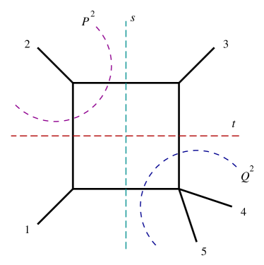
Figure 9: One of the box functions appearing in the expression of the one-loop amplitude ${\cal M}^{1-{\rm loop}}(1^{-}2^{-}3^{+}4^{+}5^{+})$.

Performing integrations in (LABEL:5p) using the result (3.50), we see that the various terms appearing in (LABEL:5p) give $P_{123}^{2}$-channel dispersion integrals of cut-boxes. A similar procedure will be followed for all the remaining MHV diagrams. One then sums over all MHV diagrams, collecting contributions to the same box function arising from the different diagrams.

As an example, let us focus on the reconstruction of the box integral in Figure 9. One needs to sum the three contributions from the function $R(31)$ in the first three terms of (LABEL:5p), and the contribution from the function $R(13)$ in the second term of (LABEL:5p). These will appear with a coefficient

$$\frac{\langle 12\rangle^{8}}{\langle 12\rangle^{2}\langle 23\rangle^{2}}\frac{[45]\ \ s_{12}s_{23}}{\langle 14\rangle\langle 15\rangle\langle 34\rangle\langle 35\rangle\langle 45\rangle}\ ,$$ (4.12)

which is precisely what expected from the result derived in [50].

One should then consider the contributions to this box function from the MHV diagrams in the null-cuts. In appendix A we argue, following [29], that specific choices of $\eta$ allow to completely discard such diagrams. Using this procedure, we have checked that our result for the five-point amplitude ${\cal M}^{1-{\rm loop}}(1^{-}2^{-}3^{+}4^{+}5^{+})$ precisely agrees with that of [50].

5 General procedure for ${n}$-point amplitudes and
conclusions

Finally, we outline a step-by-step procedure which can be applied to deal with MHV diagrams corresponding to MHV amplitudes with an arbitrary number of particles.

The building blocks of the new set of diagrammatic rules are gravity MHV amplitudes, appropriately continued to off-shell vertices. MHV amplitudes of gravitons are not holomorphic in the spinor variables, hence in section 2 we have supplied a prescription for associating spinors – specifically the anti-holomorphic spinors – to the loop momenta. This prescription is defined by certain shifts (2), which we rewrite here for convenience:

$$\hat{\tilde{l}}_{1}\ =\ \tilde{l}_{1}-z\,\frac{\langle l_{2}\eta\rangle}{\langle l_{1}l_{2}\rangle}\,\tilde{\eta}\ ,$$

$$\hat{\tilde{l}}_{2}\ =\ \tilde{l}_{2}-z\,\frac{\langle l_{1}\eta\rangle}{\langle l_{1}l_{2}\rangle}\,\tilde{\eta}\ .$$ (5.1)

These shifts are engineered in such a way to preserve momentum conservation at the MHV vertices, and therefore give us the possibility of choosing as MHV vertex any of the equivalent forms of the tree-level amplitudes. The calculation of a one-loop MHV amplitude with an arbitrary number of external legs is a straightforward generalisation of the four- and five-graviton cases discussed earlier, and proceeds along the following steps:

1. Write the expressions for all relevant MHV diagrams, using tree-level MHV vertices with shifted loop momenta given by (2). The expression for these vertices can be obtained by e.g. applying the appropriate KLT relations. When required, sum over the particles of the supermultiplet which can run in the loop.

2. If a diagram has a null two-particle cut, one applies momentum conservation of the three-point amplitude in order to cancel the presence of unphysical double poles. Our calculations (and similar ones in Yang-Mills [29, 37, 38]) show that these diagrams give a zero contribution upon choosing the gauge in an appropriate way; thus they can be discarded (see appendix A for a discussion of this point).

3. Use momentum conservation (with the shifts in place) in order to eliminate any dependence on shifted momenta. Once the integral is expressed entirely in terms of unshifted quantities, one can apply any reduction technique in order to produce an expansion in terms of boxes and, possibly, bubbles and triangles (which in ${\cal N}=8$ should cancel [19]).

4. Perform the dispersive integrations as in section 3.3, sum contributions from all MHV diagrams which can be built from MHV vertices, and finally reconstruct each box as a sum of four dispersion integrals – in its $s$-, $t$-, $P^{2}$- and $Q^{2}$-channels, using (3.60).

Clearly, it would be desirable to derive our prescription to continue off shell the loop momenta from first principles. In particular, it would be very interesting to find a derivation of the MHV diagram method in gravity similar to that of [8, 9], by performing an appropriate change of variables which would map the lightcone gravity action of [57] into an infinite sum of vertices, local in lightcone time, each with the MHV helicity structure. It would also be interesting if the MHV diagram description for gravity could be related, at least heuristically, to twistor string formulations of supergravity theories, such as those considered in [58]. We also notice that using the same shifts as in (5.1), one should be able to perform a calculation of one-loop MHV amplitudes of gravitons in theories with less supersymmetry. For pure gravity, rational terms in the amplitudes are not a priori correctly reproduced by the MHV diagram method, similarly to non-supersymmetric Yang-Mills. For instance, pure gravity has an infinite sequence of all-plus graviton amplitudes which are finite and rational. As for the the all-plus gluon amplitudes in non-supersymmetric Yang-Mills theory, it is conceivable that the all-plus graviton amplitudes arise in the MHV diagram method through violations of the $S$-matrix equivalence theorem in dimensional regularisation [45], or from four-dimensional helicity-violating counterterms as in [46].

A Comments on diagrams with null cuts

In this appendix we would like to reconsider the contributions to the MHV amplitudes arising from MHV diagrams with a null two-particle cut.

An example is the MHV diagram in Figure 10, contributing to the five-point MHV amplitude discussed in section 4. The expression for this diagrams is

$${\cal M}^{1-{\rm loop}}\ =\ \int\!d\mu_{k_{5}}\ {\cal M}(-\hat{l}_{1}^{+}1^{-}2^{-}3^{+}\hat{l}_{2}^{+}4^{+})\ {\cal M}(\hat{l}_{1}^{-}-\hat{l}_{2}^{-}5^{+})\ .$$ (A.1)

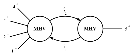
Figure 10: MHV diagram with null two-particle cut contributing to the five-point graviton MHV amplitude at one loop.

Using KLT relations for six- (C) and for three-graviton amplitudes (C.1), we can write (A.1) as a sum of two terms plus permutations of the particles ${\cal P}(123)$. Similarly to section 3.2, momentum conservation $k_{5}-\hat{l}_{2}+\hat{l}_{1}=0$ allows to prove easily the cancellation of unphysical double poles appearing because of the presence of a three-point graviton vertex. Furthermore, all the dependence on hatted quantities can be eliminated using momentum conservation in the form

$$\langle l_{1}l_{2}\rangle[\hat{l}_{2}i]\ =\ \langle l_{1}5\rangle[5i]\ ,\qquad\langle l_{2}l_{1}\rangle[\hat{l}_{1}j]\ =\ -\langle l_{2}5\rangle[5j]\ .$$ (A.2)

Following this procedure, the starting expression (A.1) is decomposed into a sum of terms, on which one easily applies PV reduction techniques. Similarly to the four-point case, one can see that only box functions in null cuts are produced.

The remark we would like to make now is that such terms actually vanish with appropriate choices of the null reference vector $\eta$, as observed in the Yang-Mills case in [29]. The same choice of $\eta$ has been used in [37, 36, 38] in deriving gluon amplitudes in Yang-Mills theory, and recently in [39, 40, 41] in deriving one-loop $\phi$-MHV amplitudes, i.e. amplitudes with gluons in an MHV helicity configuration and a complex scalar $\phi$ coupled to the gluons via the interaction $\phi\,{\rm Tr}F_{\mu\nu}F^{\mu\nu}$.

In [29], it was found how a generic two-mass easy box function is reconstructed by summing over four dispersion integrals, as in (3.60). These dispersion integrals are performed in the four channels $s$, $t$, $P^{2}$ and $Q^{2}$ of the box function. As explained in that paper, the evaluation of these integrals is greatly facilitated by choosing the reference vector $\eta$ appearing in (2.1) to be one of the two massless momenta, $p$ and $q$, of the box function (see Figure 5 for the labeling of the momenta in a generic two-mass easy box). By performing this choice, one finds that the contribution of a single dispersion integral of a cut-box in a generic cut $s_{\rm cut}$ is proportional, to all orders in the dimensional regularisation parameter $\epsilon$, to [33]

$$-\frac{c_{\Gamma}}{\epsilon^{2}}(-s_{\rm cut})^{-\epsilon}\,{}_{2}F_{1}(1,-\epsilon,1-\epsilon,as_{\rm cut})\ ,$$ (A.3)

where $c_{\Gamma}$ is defined in (3.52) and $a$ is defined in (3.47). In the four-point box function, one obviously has $P^{2}=Q^{2}=0$. Using (A.3), it is then immediate to see that the dispersion integrals in these two channels vanish because of the presence of the factor $(-s_{\rm cut})^{-\epsilon}$. Therefore, when summing over all the possible MHV diagrams, it is in fact enough to consider only the MHV diagrams with non-vanishing cuts.

Finally, we notice that for arbitrary choices of $\eta$, this would no longer be true; the MHV diagrams in null channels would be important to restore $\eta$-independence in the final expressions of one-loop amplitudes.

As a side remark, it instructive to apply the above comments to rederive with MHV diagrams, almost instantly, the expression to all orders in the dimensional regularisation parameter, $\epsilon$, of the one-loop four-gluon amplitude in ${\cal N}=4$ super Yang-Mills. In this case, the result comes from summing two dispersion integrals, namely those in the $s=(k_{1}+k_{2})^{2}$ and in the $t=(k_{2}+k_{3})^{2}$ channels; indeed, the specific choices of $\eta$ mentioned above allow us to discard the MHV diagrams with null two-particle cut. In the four-particle case, the expression for $a$ in (3.47) simplifies to $a|_{P^{2}=Q^{2}=0}=1/s+1/t$. One then quickly obtains, to all orders in $\epsilon$ [33],

$${\cal A}^{1-{\rm loop}}\ =\ 2{\cal A}^{\rm tree}\,\frac{c_{\Gamma}}{\epsilon^{2}}\left[(-s)^{-\epsilon}{}_{2}F_{1}\left(1,-\epsilon,1-\epsilon,1+\frac{s}{t}\right)+(-t)^{-\epsilon}{}_{2}F_{1}\left(1,-\epsilon,1-\epsilon,1+\frac{t}{s}\right)\right]\ .$$ (A.4)

(A.4) agrees with the known result [47].

B Reduction technique of the $R$-functions

In dealing with expressions of gravity amplitudes derived using the MHV diagram method, one often encounters products of “$R$-functions”, where

$$R(ij)\ =\ \frac{\langle il_{2}\rangle\langle jl_{1}\rangle}{\langle il_{1}\rangle\langle jl_{2}\rangle}\ .$$ (B.1)

The appearance of products of these functions is related to the structure of tree-level gravity amplitudes, which can be expressed, using KLT relations, as sums of products of two Yang-Mills amplitudes. Here we would like to discuss how to reduce products of $R$-functions to sums of $R$-functions and bubbles.

To begin with, we observe some useful properties of these functions:

$$R(ab)R(bc)\ =\ R(ac)\ \Rightarrow\ R(ab)R(ba)\ =\ 1\ ,$$ (B.2)

(B.3)

$$R(ab)R(cd)\ =\ R(ad)R(cb)\ \Rightarrow\ R(ab)R(da)\ =\ R(db)\ .$$ (B.4)

Let us now consider a generic product $R(ij)R(hk)$ with $i\neq j\neq h\neq k$,

$$R(ij)R(hk)\ =\ \frac{\langle il_{2}\rangle\langle jl_{1}\rangle}{\langle il_{1}\rangle\langle jl_{2}\rangle}\frac{\langle hl_{2}\rangle\langle kl_{1}\rangle}{\langle hl_{1}\rangle\langle kl_{2}\rangle}\ .$$ (B.5)

Using Schouten’s identity in the form

$$\frac{\langle al\rangle}{\langle bl\rangle\langle cl\rangle}\ =\ \frac{\langle ac\rangle}{\langle bc\rangle}\frac{1}{\langle cl\rangle}+\frac{\langle ba\rangle}{\langle bc\rangle}\frac{1}{\langle bl\rangle}\ ,$$ (B.6)

one can separate contributions from different poles. Applying this to the two ratios $\langle kl_{1}\rangle/(\langle il_{1}\rangle\langle hl_{1}\rangle)$ and $\langle hl_{2}\rangle/(\langle jl_{2}\rangle\langle kl_{2}\rangle)$, we get

$$R(ij)R(hk)\ =\ \frac{\langle ik\rangle\langle jh\rangle}{\langle ih\rangle\langle jk\rangle}R(ij)+\frac{\langle hk\rangle}{\langle ih\rangle\langle jk\rangle}\left[\langle kh\rangle\frac{\mathcal{K}(ij)}{\mathcal{K}(kh)}+\langle hj\rangle\frac{\mathcal{K}(ij)}{\mathcal{K}(jh)}+\langle ik\rangle\frac{\mathcal{K}(ij)}{\mathcal{K}(ki)}\right]\ ,$$ (B.7)

where we have defined

$$\mathcal{K}(ij)\ :=\ \langle il_{2}\rangle\langle jl_{1}\rangle\ .$$ (B.8)

Notice that $R(ij)$ can be expressed in terms of $\mathcal{K}_{ij}$ as

$$R(ij)\ =\ \frac{\mathcal{K}(ij)}{\mathcal{K}(ji)}$$ (B.9)

We can use again the same decomposition on a generic term

$$\frac{\mathcal{K}(ij)}{\mathcal{K}(hk)}\ =\ \frac{\langle il_{2}\rangle\langle jl_{1}\rangle}{\langle hl_{2}\rangle\langle kl_{1}\rangle}\frac{\langle hl_{1}\rangle}{\langle hl_{1}\rangle}\frac{\langle kl_{2}\rangle}{\langle kl_{2}\rangle}\ ,$$ (B.10)

to get

$$\frac{\mathcal{K}(ij)}{\mathcal{K}(hk)}\ =\ \frac{\langle kj\rangle\langle hi\rangle}{\langle kh\rangle\langle hk\rangle}R(kh)+\frac{1}{\langle kh\rangle\langle hk\rangle}\left[\langle jh\rangle\langle ik\rangle+\langle jh\rangle\langle hi\rangle\frac{\langle kl_{2}\rangle}{\langle hl_{2}\rangle}+\langle kj\rangle\langle ik\rangle\frac{\langle hl_{1}\rangle}{\langle kl_{1}\rangle}\right]\ .$$ (B.11)

By substituting this expression into (B.7), we see that we are left with a bubble plus the sum of $R$-functions. Using the Schouten identity, we arrive at the final result

$$R(ij)R(hk)\ =\ -1+\frac{\langle hk\rangle\langle ij\rangle}{\langle ih\rangle\langle jk\rangle}\left[R(hj)+R(ik)\right]+\frac{\langle ik\rangle\langle jh\rangle}{\langle ih\rangle\langle jk\rangle}\left[R(ij)+R(hk)\right]\ .$$ (B.12)

This formula allows us to perform immediately PV reductions of $R$-functions. Further reducing the $R$-functions as usual (3.3), we are then left with bubbles, triangles and boxes.

C KLT relations

For completeness, in this appendix we include the field theory limit expressions of the KLT relations [56] for the case of four-, five- and six-point amplitudes. These are,

$${\cal M}(1,2,3) = -i{\cal A}(1,2,3)\,{\cal A}(1,2,3)\ ,$$ (C.1)

$${\cal M}(1,2,3,4) = -is_{12}\ {\cal A}(1,2,3,4){\cal A}(1,2,4,3)\ ,$$ (C.3)

$${\cal M}(1,2,3,4,5) = is_{12}s_{34}\ {\cal A}(1,2,3,4,5){\cal A}(2,1,4,3,5)$$ (C.4)

$$+ is_{13}s_{24}\ {\cal A}(1,3,2,4,5){\cal A}(3,1,4,2,5)\ ,$$

$${\cal M}(1,2,3,4,5,6) = -is_{12}s_{45}\ {\cal A}(1,2,3,4,5,6)\big{[}s_{35}{\cal A}(2,1,5,3,4,6)$$

$$+ (s_{34}+s_{35})\ {\cal A}(2,1,5,4,3,6)\big{]}$$

$$+ {\cal P}(2,3,4)\ .$$

In these formulae, ${\cal M}$ (${\cal A}$) denotes a tree-level gravity (Yang-Mills, colour-ordered) amplitude, $s_{ij}:=(k_{i}+k_{j})^{2}$, and ${\cal P}(2,3,4)$ stands for permutations of $(2,3,4)$. The form of KLT relations for a generic number of particles can be found in [50].

References

- [1] E. Witten, Perturbative gauge theory as a string theory in twistor space, Commun. Math. Phys. 252, 189 (2004), hep-th/0312171.
- [2] F. Cachazo and P. Svrček, Lectures on twistor strings and perturbative Yang-Mills theory, PoS RTN2005, 004 (2005), hep-th/0504194.
- [3] F. Cachazo, P. Svrček and E. Witten, MHV vertices and tree amplitudes in gauge theory, JHEP 0409 (2004) 006, hep-th/0403047.
- [4] G. Georgiou and V. V. Khoze, Tree amplitudes in gauge theory as scalar MHV diagrams, JHEP 0405 (2004) 070 hep-th/0404072.
- [5] J. B. Wu and C. J. Zhu, MHV vertices and fermionic scattering amplitudes in gauge theory with quarks and gluinos, JHEP 0409 (2004) 063 hep-th/0406146.
- [6] J. B. Wu and C. J. Zhu, MHV vertices and scattering amplitudes in gauge theory, JHEP 0407 (2004) 032, hep-th/0406085.
- [7] G. Georgiou, E. W. N. Glover and V. V. Khoze, Non-MHV tree amplitudes in gauge theory, JHEP 0407 (2004) 048, hep-th/0407027.
- [8] P. Mansfield, The Lagrangian origin of MHV rules, JHEP 0603 (2006) 037, hep-th/0511264.
- [9] A. Gorsky and A. Rosly, From Yang-Mills Lagrangian to MHV diagrams, JHEP 0601 (2006) 101, hep-th/0510111.
- [10] J. H. Ettle and T. R. Morris, Structure of the MHV-rules Lagrangian, JHEP 0608, 003 (2006), hep-th/0605121.
- [11] R. Boels, L. Mason and D. Skinner, From twistor actions to MHV diagrams, Phys. Lett. B 648 (2007) 90, hep-th/0702035.
- [12] R. Britto, F. Cachazo and B. Feng, New recursion relations for tree amplitudes of gluons, Nucl. Phys. B 715, 499 (2005) hep-th/0412308.
- [13] R. Britto, F. Cachazo, B. Feng and E. Witten, Direct proof of tree-level recursion relation in Yang-Mills theory, Phys. Rev. Lett. 94 (2005) 181602, hep-th/0501052.
- [14] J. Bedford, A. Brandhuber, B. Spence and G. Travaglini, A recursion relation for gravity amplitudes, Nucl. Phys. B 721, 98 (2005), hep-th/0502146.
- [15] F. Cachazo and P. Svrček, Tree level recursion relations in general relativity, hep-th/0502160.
- [16] A. Brandhuber, S. McNamara, B. Spence and G. Travaglini, Recursion relations for one-loop gravity amplitudes, JHEP 0703 (2007) 029, hep-th/0701187.
- [17] P. Benincasa, C. Boucher-Veronneau and F. Cachazo, Taming tree amplitudes in general relativity, hep-th/0702032.
- [18] N. E. J. Bjerrum-Bohr, D. C. Dunbar and H. Ita, Six-point one-loop N = 8 supergravity NMHV amplitudes and their IR behaviour, Phys. Lett. B 621 (2005) 183, hep-th/0503102.
- [19] N. E. J. Bjerrum-Bohr, D. C. Dunbar, H. Ita, W. B. Perkins and K. Risager, The no-triangle hypothesis for N = 8 supergravity, JHEP 0612 (2006) 072, hep-th/0610043.
- [20] Z. Bern, N. E. J. Bjerrum-Bohr and D. C. Dunbar, Inherited twistor-space structure of gravity loop amplitudes, JHEP 0505 (2005) 056, hep-th/0501137.
- [21] M. B. Green, J. G. Russo and P. Vanhove, Non-renormalisation conditions in type II string theory and maximal supergravity, hep-th/0610299.
- [22] Z. Bern, L. J. Dixon and R. Roiban, Is N = 8 supergravity ultraviolet finite?, hep-th/0611086.
- [23] M. B. Green, J. G. Russo and P. Vanhove, Ultraviolet properties of maximal supergravity, hep-th/0611273.
- [24] Z. Bern, J. J. Carrasco, L. J. Dixon, H. Johansson, D. A. Kosower and R. Roiban, Three-loop superfiniteness of N = 8 supergravity, hep-th/0702112.
- [25] G. Chalmers, On the finiteness of N = 8 quantum supergravity, hep-th/0008162.
- [26] N. E. J. Bjerrum-Bohr, D. C. Dunbar, H. Ita, W. B. Perkins and K. Risager, MHV-vertices for gravity amplitudes, JHEP 0601 (2006) 009, hep-th/0509016.
- [27] S. Giombi, R. Ricci, D. Robles-Llana and D. Trancanelli, A note on twistor gravity amplitudes, JHEP 0407 (2004) 059, hep-th/0405086.
- [28] K. Risager, A direct proof of the CSW rules, JHEP 0512 (2005) 003, hep-th/0508206.
- [29] A. Brandhuber, B. Spence and G. Travaglini, One-Loop Gauge Theory Amplitudes in N=4 super Yang-Mills from MHV Vertices, Nucl. Phys. B 706 (2005) 150, hep-th/0407214.
- [30] A. Brandhuber and G. Travaglini, Quantum MHV diagrams, hep-th/0609011.
- [31] Z. Bern, L. J. Dixon, D. C. Dunbar and D. A. Kosower, Fusing gauge theory tree amplitudes into loop amplitudes, Nucl. Phys. B 435 (1995) 59, hep-ph/9409265.
- [32] Z. Bern, L. J. Dixon, D. C. Dunbar and D. A. Kosower, One loop n point gauge theory amplitudes, unitarity and collinear limits, Nucl. Phys. B 425 (1994) 217, hep-ph/9403226.
- [33] A. Brandhuber, B. Spence and G. Travaglini, From trees to loops and back, JHEP 0601 (2006) 142, hep-th/0510253.
- [34] R. P. Feynman, Quantum Theory Of Gravitation, Acta Phys. Polon. 24 (1963) 697.
- [35] R. P. Feynman, Closed Loop And Tree Diagrams, in J. R. Klauder, Magic Without Magic, San Francisco 1972, 355-375; in Brown, L. M. (ed.): Selected papers of Richard Feynman, 867-887
- [36] C. Quigley and M. Rozali, One-Loop MHV Amplitudes in Supersymmetric Gauge Theories, JHEP 0501 (2005) 053, hep-th/0410278.
- [37] J. Bedford, A. Brandhuber, B. Spence and G. Travaglini, A Twistor Approach to One-Loop Amplitudes in Supersymmetric Yang-Mills Theory, Nucl. Phys. B 706 (2005) 100, hep-th/0410280.
- [38] J. Bedford, A. Brandhuber, B. Spence and G. Travaglini, Non-supersymmetric loop amplitudes and MHV vertices, Nucl. Phys. B 712 (2005) 59, hep-th/0412108.
- [39] S. D. Badger and E. W. N. Glover, One-loop helicity amplitudes for H gluons: The all-minus configuration, Nucl. Phys. Proc. Suppl. 160 (2006) 71, hep-ph/0607139.
- [40] S. D. Badger, E. W. N. Glover and K. Risager, One-loop phi-MHV amplitudes using the unitarity bootstrap, 0704.3914 [hep-ph].
- [41] S. D. Badger, E. W. N. Glover and K. Risager, Higgs amplitudes from twistor inspired methods, 0705.0264 [hep-ph].
- [42] L. J. Dixon, E. W. N. Glover and V. V. Khoze, MHV rules for Higgs plus multi-gluon amplitudes, JHEP 0412 (2004) 015, hep-th/0411092.
- [43] S. D. Badger, E. W. N. Glover and V. V. Khoze, MHV rules for Higgs plus multi-parton amplitudes, JHEP 0503 (2005) 023, hep-th/0412275.
- [44] A. Brandhuber, B. Spence and G. Travaglini, Amplitudes in pure Yang-Mills and MHV diagrams, JHEP 0702 (2002) 88, hep-th/0612007.
- [45] J. H. Ettle, C. H. Fu, J. P. Fudger, P. R. W. Mansfield and T. R. Morris, S-Matrix Equivalence Theorem Evasion and Dimensional Regularisation with the Canonical MHV Lagrangian, hep-th/0703286.
- [46] A. Brandhuber, B. Spence, G. Travaglini and K. Zoubos, One-loop MHV Rules and Pure Yang-Mills, 0704.0245 [hep-th].
- [47] M. B. Green, J. H. Schwarz and L. Brink, N=4 Yang-Mills And N=8 Supergravity As Limits Of String Theories, Nucl. Phys. B 198 (1982) 474.
- [48] D. C. Dunbar and P. S. Norridge, Calculation of graviton scattering amplitudes using string based methods, Nucl. Phys. B 433, 181 (1995), hep-th/9408014.
- [49] Z. Bern and D. A. Kosower, The Computation of loop amplitudes in gauge theories, Nucl. Phys. B 379 (1992) 451.
- [50] Z. Bern, L. J. Dixon, M. Perelstein and J. S. Rozowsky, Multi-leg one-loop gravity amplitudes from gauge theory, Nucl. Phys. B 546 (1999) 423, hep-th/9811140.
- [51] Z. Bern, Perturbative quantum gravity and its relation to gauge theory, Living Rev. Rel. 5, 5 (2002) gr-qc/0206071.
- [52] D. A. Kosower, Next-to-maximal helicity violating amplitudes in gauge theory, Phys. Rev. D 71 (2005) 045007, hep-th/0406175.
- [53] F. A. Berends, W. T. Giele and H. Kuijf, On relations between multi-gluon and multigraviton scattering, Phys. Lett. B 211 (1988) 91.
- [54] M. L. Mangano and S. J. Parke, Multiparton amplitudes in gauge theories, Phys. Rept. 200 (1991) 301, hep-th/0509223.
- [55] M. T. Grisaru, H. N. Pendleton and P. van Nieuwenhuizen, Supergravity And The S Matrix, Phys. Rev. D 15 (1977) 996.
- [56] H. Kawai, D. C. Lewellen and S. H. H. Tye, A Relation Between Tree Amplitudes Of Closed And Open Strings, Nucl. Phys. B 269 (1986) 1.
- [57] J. Scherk and J. H. Schwarz, Gravitation In The Light - Cone Gauge, Gen. Rel. Grav. 6 (1975) 537.
- [58] M. Abou-Zeid, C. M. Hull and L. J. Mason, Einstein supergravity and new twistor string theories, hep-th/0606272.