Quiver Gauge Theory and Noncommutative Vortices

Abstract

We construct explicit BPS and non-BPS solutions of the Yang-Mills equations on noncommutative spaces ${\mathbb{R}}^{2n}_{\theta}\times G/H$ which are manifestly $G$-symmetric. Given a $G$-representation, by twisting with a particular bundle over $G/H$, we obtain a $G$-equivariant U($k$) bundle with a $G$-equivariant connection over ${\mathbb{R}}^{2n}_{\theta}\times G/H$. The U($k$) Donaldson-Uhlenbeck-Yau equations on these spaces reduce to vortex-type equations in a particular quiver gauge theory on ${\mathbb{R}}^{2n}_{\theta}$. Seiberg-Witten monopole equations are particular examples. The noncommutative BPS configurations are formulated with partial isometries, which are obtained from an equivariant Atiyah-Bott-Shapiro construction. They can be interpreted as D0-branes inside a space-filling brane-antibrane system.
Talk by O.L. at the 21st Nishinomiya-Yukawa Memorial Symposium, Kyoto, 15 Nov. 2006

1 Twisted dimensional reduction

It is an old dream to “explain” the standard model of particle physics by dimensional reduction of a higher-dimensional gauge theory. After the reduction, the field dependence on the extra coordinates must of course disappear from the four-dimensional Lagrangian. Usually, this is achieved, in a rather crude way, by simply discarding the fields’ dependence on the extra coordinates. However, independence is by no means necessary: it suffices to prescribe some dependence, like, e.g., in warped compactifications. If the extra spacetime dimensions admit isometries, it is particularly elegant to compensate these by gauge transformations. In this way, the Lie derivative with respect to a Killing vector becomes a gauge generator. The bonus is a unification of gauge and Higgs sectors in the higher-dimensional gauge theory.

The natural setting for spacetime isometries are coset spaces $G/H$, and thus one is led to a reduction ${\mathcal{M}}\times\frac{G}{H}\ \longrightarrow\ {\mathcal{M}}$ where the manifold ${\mathcal{M}}$ is to be specified later. Such a “coset-space dimensional reduction” [1] was first suggested by Witten,[2] Forgacs and Manton,[3, 4] and has since been extended supersymmetrically[5] and embedded into superstring theory.[6]  In the present talk, for Lie groups $G$ of rank one and rank two, we shall apply this scheme to perform a $G$-equivariant reduction of Yang-Mills theory over $G/H$ to a quiver gauge theory on ${\mathcal{M}}$,[7, 8, 9, 10] formulate its BPS equations and show how to construct a certain class of solutions, which admit a D-brane interpretation. These solutions, however, only exist when the system is subjected to a noncommutative deformation. Therefore, about half-way into the talk we specialize to ${\mathcal{M}}={\mathbb{C}}^{n}$ and apply a Moyal deformation. Most material presented here has appeared in Refs. Lechtenfeld:2003cq,Popov:2005ik,Lechtenfeld:2006wu, some is work in progress.

2 Kähler times coset space $G/H$

To be concrete, let us consider U($k$) Yang-Mills theory on ${\mathcal{M}}_{2n}\times\frac{G}{H}$, with ${\mathcal{M}}_{2n}$ being a real $2n$-dimensional Kähler manifold with Kähler form  $\omega$  and metric  $g$. For cosets, we shall examine the following four examples:
$G/H$: ${\mathbb{C}}P^{1}$ ${\mathbb{C}}P^{1}\times{\mathbb{C}}P^{1}$ ${\mathbb{C}}P^{2}$ $Q_{3}$ $\|$ $\|$ $\|$ $\|$  $\frac{\mathrm{SU}(2)}{\mathrm{U}(1)}$  $\frac{\mathrm{SU}(2)\times\mathrm{SU}(2)}{\mathrm{U}(1)\times\mathrm{U}(1)}$  $\frac{\mathrm{SU}(3)}{\mathrm{S}(\mathrm{U}(2)\times\mathrm{U}(1))}$  $\frac{\mathrm{SU}(3)}{\mathrm{U}(1)\times\mathrm{U}(1)}$ $d{=}2$ $d{=}4$ $d{=}4$ $d{=}6$
These are homogeneous but not necessarily symmetric spaces ($Q_{3}$ is not). Furthermore, they are Kähler, with Kähler forms $\beta\wedge\bar{\beta}$ factorized into canonical one-forms.

3 Donaldson-Uhlenbeck-Yau equations

To formulate U($k$) Yang-Mills theory on ${\mathcal{M}}_{2n}\times\frac{G}{H}$, we introduce a rank-$k$ hermitian vector bundle

$$\begin{CD}{\mathcal{E}}\\ @V{}V{{\mathbb{C}}^{k}}V\\ {\mathcal{M}}_{2n}\times\frac{G}{H}\end{CD}$$ (1)

with structure group $\mathrm{U}(k)$ and a connection ${\mathcal{A}}$ which gives rise to the curvature or field strength  ${\mathcal{F}}\ =\ \mathrm{d}{\mathcal{A}}+{\mathcal{A}}\wedge{\mathcal{A}}$  subject to the Bianchi identity  $D_{\!{\mathcal{A}}}\,{\mathcal{F}}=0$  where $D_{\!{\mathcal{A}}}$ is the gauge covariant derivative.

The (vacuum) Yang-Mills equations read

$$D_{\!{\mathcal{A}}}\,(*{\mathcal{F}})\ =\ 0$$ (2)

where ‘$*$’ denotes the Hodge dual. With respect to the Kähler form $\Omega=\omega+\beta{\wedge}\bar{\beta}$ of the total space, the field strength decomposes as

$${\mathcal{F}}\ =\ {\mathcal{F}}^{(2,0)}\ +\ {\mathcal{F}}^{(1,1)}\ +\ {\mathcal{F}}^{(0,2)}\ .$$ (3)

So-called stable bundles ${\mathcal{E}}$ solve the Donaldson-Uhlenbeck-Yau equations [14, 15]

$${\mathcal{F}}^{(2,0)}\ =\ 0\ =\ {\mathcal{F}}^{(0,2)}\qquad\text{and}\qquad*\Omega\wedge{\mathcal{F}}\ =\ 0\qquad\qquad\text{(DUY)}$$ (4)

which are first-order conditions on the connection ${\mathcal{A}}$. Their importance derives from the fact that the $n^{2}{-}n{+}1$ DUY equations imply the $2n$ full Yang-Mills equations (2). Hence, for obtaining classical solutions it suffices to solve the DUY equations rather than the full second-order field equations (but it is by no means necessary). As a special case, on ${\mathcal{M}}_{4}$ ($n{=}2$) the 3 DUY equations reduce to the famous self-duality equations $F=*F$ which yield instantons and monopoles.

4 $G$-equivariant bundle construction

In order to implement the coset-space reduction, we must construct a $G$-equivariant bundle over the coset space. A rank-$d$ vector bundle  ${\mathcal{L}}\buildrel{\mathbb{C}}^{d}\over{\longrightarrow}G/H$  with structure group U($d$) is $G$-equivariant if the left translations $L_{g}$ on ${\mathcal{L}}$ (with $g\in G$) are compatible with the right U($d$) action and the following diagram is commutative,

$$\begin{CD}{\mathcal{L}}@>{L_{g}}>{}>{\mathcal{L}}\\ @V{}V{\pi}V@V{\pi}V{}V\\ \frac{G}{H}@>{l_{g}}>{}>\frac{G}{H}\end{CD}\quad,$$ (5)

where $l_{g}$ is the left translation on the coset space. Since $L_{h}\in\mathrm{U}(d)$ for $h\in H$, this defines a representation $\rho:H\hookrightarrow\mathrm{U}(d)$. For simplicity, we take $\rho$ to be irreducible.

As a next step, we extend the bundle ${\mathcal{L}}$ by a rank-$k$ vector bundle $E$ over ${\mathcal{M}}_{2n}$,

$$\begin{CD}{\mathcal{L}}\\ @V{}V{{\mathbb{C}}^{d}}V\\ \frac{G}{H}\end{CD}\qquad\longrightarrow\quad\begin{CD}E\otimes{\mathcal{L}}\\ @V{}V{{\mathbb{C}}^{k}\otimes{\mathbb{C}}^{d}}V\\ {\mathcal{M}}_{2n}\times\frac{G}{H}\end{CD}\qquad,$$ (6)

to a bundle over the total space with a trivial $G$-action on $E$. Further, we form a Whitney sum of $m{+}1$ such bundles with data $(k_{i},d_{i},\rho_{i})$ for $i=0,1,\dots,m$. The $G$-equivariant total bundle

$${\mathcal{E}}\ =\ \bigoplus_{i=0}^{m}E_{i}\otimes{\mathcal{L}}_{i}$$ (7)

comes with a structure group $\prod_{i}\mathrm{U}(k_{i})\times\mathrm{U}(d_{i})$ and admits $G$-equivariant connections ${\mathcal{A}}$ (i.e. connections compatible with equivariance).

5 $G$-equivariant connection

Finally, we twist each subbundle  $E_{i}\buildrel{\mathbb{C}}^{k_{i}}\over{\longrightarrow}{\mathcal{M}}_{2n}$  with a connection  $A^{i}\in u(k_{i})$  by the homogeneous bundle  ${\mathcal{L}}_{i}\buildrel{\mathbb{C}}^{d_{i}}\over{\longrightarrow}G/H$  with a connection $a^{i}$ in the Lie$H$-irrep $\rho_{i}$. Hence, the connection on $E_{i}\otimes{\mathcal{L}}_{i}$ reads

$${\mathcal{A}}^{i}\ =\ A^{i}\otimes\boldsymbol{1}_{d_{i}}\ +\ \boldsymbol{1}_{k_{i}}\otimes a^{i}\qquad\text{for}\quad i=0,1,\ldots,m\ .$$ (8)

It is important to realize that the $G$-action connects different $H$-irreps, $\rho_{i}\buildrel g\over{\to}\rho_{j}$, so that the total connection

$${\mathcal{A}}\ =\ \bigoplus_{i=0}^{m}{\mathcal{A}}^{i}\ +\ \text{``off-diagonal''}$$ (9)

is not block-diagonal. $G$-equivariance then dictates the decomposition of the connection into $k_{i}d_{i}{\times}k_{j}d_{j}$ blocks as

$${\mathcal{A}}\ =\ \begin{pmatrix}A^{0}{\otimes}\boldsymbol{1}_{d_{0}}+\boldsymbol{1}_{k_{0}}{\otimes}\,a^{0}&\phi_{01}\otimes\beta_{01}&\cdots&\phi_{0m}\otimes\beta_{0m}\\[16.0pt] \phi_{10}\otimes\beta_{10}&A^{1}{\otimes}\boldsymbol{1}_{d_{1}}+\boldsymbol{1}_{k_{1}}{\otimes}\,a^{1}&\cdots&\phi_{1m}\otimes\beta_{1m}\\[16.0pt] \vdots&\vdots&\ddots&\vdots\\[16.0pt] \phi_{m0}\otimes\beta_{m0}&\phi_{m1}\otimes\beta_{m1}&\cdots&A^{m}{\otimes}\boldsymbol{1}_{d_{m}}+\boldsymbol{1}_{k_{m}}{\otimes}\,a^{m}\end{pmatrix}$$ (10)

with size $k_{i}{\times}k_{j}$ Higgs fields

$$\phi_{ij}\ =\ \phi^{\dagger}_{ji}\ \in\mathrm{Hom}({\mathbb{C}}^{k_{j}},{\mathbb{C}}^{k_{i}})$$ (11)

in the bi-fundamental representation of $\mathrm{U}(k_{i})\times\mathrm{U}(k_{j})$ and size $d_{i}{\times}d_{j}$ one-forms  $\beta_{ij}=-\beta^{\dagger}_{ji}$  on $\frac{G}{H}$ built from the components of $\beta$ and $\bar{\beta}$.

This construction breaks the original gauge group

$$\mathrm{U}({\textstyle\sum}_{i}k_{i}d_{i})\ \longrightarrow\ \prod_{i}\mathrm{U}(k_{i})$$ (12)

via the Higgs effect. In the following we choose the collection  $\{\rho_{i}\}$  to descend from some $G$-irrep ${\mathcal{D}}$, i.e.

$${\mathcal{D}}|_{{}_{H}}\ =\ \bigoplus_{i=0}^{m}\rho_{i}\ .$$ (13)

It should be noted that the coset generators connect only particular pairs $(\rho_{j},\rho_{i})$ so that many one-forms $\beta_{ij}$ actually vanish.

6 The quiver diagram

The connection  ${\mathcal{A}}\ \sim\ \{A^{i},\phi_{ij}\}$  realizes a quiver gauge theory: For each $H$-irrep $\rho_{i}$ draw one vertex, which carries a multiplicity space ${\mathbb{C}}^{k_{i}}$ and a connection $A^{i}\in u(k_{i})$; for each nonzero one-form $\beta_{ij}:\rho_{j}\to\rho_{i}$ draw an arrow from vertex $j$ to vertex $i$, which carries a Higgs field $\phi_{ij}:{\mathbb{C}}^{k_{j}}\to{\mathbb{C}}^{k_{i}}$. Abbreviating $\phi_{ij}\otimes\beta_{ij}=:\Phi_{ij}$ we obtain pictorially

$$\cdots\ \buildrel i\over{\bullet}\ \ \buildrel\Phi_{ij}\over{\longleftarrow}\ \ \buildrel j\over{\bullet}\ \cdots$$ (14)

as the building block for a quiver diagram. The most general such diagram may in fact be obtained from the above construction by deleting some of the vertices (and connecting arrows).[10] In the following, we discuss examples based on $G$ of rank one and rank two.

7 Rank-one example

We come to the basic example of

$$\frac{G}{H}\ \cong\ \frac{\mathrm{SU}(2)}{\mathrm{U}(1)}\ \cong\ S^{2}_{R}\qquad\text{with}\qquad\beta\ =\ \frac{2R^{2}\mathrm{d}y}{R^{2}+y\bar{y}}\ ,$$ (15)

where $R$ is the radius of the two-sphere and $y$ denotes its (complex) stereographic coordinate.

The homogeneous bundle in question is the $q$-monopole bundle

$${\mathcal{L}}^{q}\ =\ {\mathcal{L}}^{\otimes q}\qquad\text{with}\qquad\begin{CD}{\mathcal{L}}{=}S^{3}\\ @V{}V{S^{1}}V\\ S^{2}_{R}\end{CD}$$ (16)

and transition functions $(\frac{y}{\bar{y}})^{\frac{q}{2}}=\mathrm{e}^{\,\mathrm{i}\,q\varphi}$. The $q$-monopole connection and field strength read

$$a_{q}\ =\ \frac{q}{2}\,\frac{\bar{y}\mathrm{d}y-y\mathrm{d}\bar{y}}{R^{2}+y\bar{y}}\qquad\longrightarrow\qquad f_{q}\ =\ -\frac{q}{4R^{2}}\,\beta\wedge\bar{\beta}\qquad\text{with}\quad c_{1}\!=\mathrm{deg}\,{\mathcal{L}}^{q}=q\ .$$ (17)

Let us pick an $\mathrm{SU}(2)$-irrep  ${\mathcal{D}}=\underline{$m{+}1$}$  (i.e. spin $\frac{m}{2}$) so that the $\mathrm{U}(1)$ irreps are characterized by charges $q_{i}=m{-}2i$ for $i=0,1,\ldots,m$, and $\beta_{ij}=0$ except for $\beta_{i\ i-1}=-\beta$ and $\beta_{i\ i+1}=\bar{\beta}$. Labelling the vertices from the highest $\mathrm{SU}(2)$ weight downwards, we get chains

$$\!\!E_{m}\buildrel\phi_{m\,m-1}\over{\longleftarrow}\!\!\cdots\buildrel\phi_{21}\over{\longleftarrow}E_{1}\buildrel\phi_{10}\over{\longleftarrow}E_{0}\qquad\text{and}\qquad{\mathcal{L}}^{-m}\buildrel\beta\over{\longleftarrow}\cdots\buildrel\beta\over{\longleftarrow}{\mathcal{L}}^{m-2}\buildrel\beta\over{\longleftarrow}{\mathcal{L}}^{m}$$ (18)

which are represented diagrammatically by the linear (or $A_{m+1}$) quiver

$$\begin{CD}\buildrel m\over{\bullet}@<{\ \!\Phi_{m\,m-1}\!}<{}<\cdots @<{\ \Phi_{32}\ }<{}<\buildrel 2\over{\bullet}@<{\ \Phi_{21}\ }<{}<\buildrel 1\over{\bullet}@<{\ \Phi_{10}\ }<{}<\buildrel 0\over{\bullet}\end{CD}\quad.$$ (19)

8 Rank-two examples

More instructive are the three rank-two examples listed in §2. First, in the product case of ${\mathbb{C}}P^{1}\times{\mathbb{C}}P^{1}\ \cong\ \frac{\mathrm{SU}(2)}{\mathrm{U}(1)}\times\frac{\mathrm{SU}(2)}{\mathrm{U}(1)}$ the $G$-irrep is given by a pair of spins, ${\mathcal{D}}\ =\ (\underline{$m_{1}{+}1$}\,,\,\underline{$m_{2}{+}1$})$ . It is obvious that the corresponding quiver becomes a product of two chains (see right). Second, for the nonsymmetric coset $\setcounter{MaxMatrixCols}{11}\begin{CD}\bullet @<{}<{}<\bullet @<{}<{}<\bullet @<{}<{}<\cdots @<{}<{}<\bullet\\ @V{}V{}V@V{}V{}V@V{}V{}V&&@V{}V{}V\\ \bullet @<{}<{}<\bullet @<{}<{}<\bullet @<{}<{}<\cdots @<{}<{}<\bullet\\ @V{}V{}V@V{}V{}V@V{}V{}V&&@V{}V{}V\\ \vdots&&\vdots&&\vdots&&&&\vdots\\ @V{}V{}V@V{}V{}V@V{}V{}V&&@V{}V{}V\\ \bullet @<{}<{}<\bullet @<{}<{}<\bullet @<{}<{}<\cdots @<{}<{}<\bullet\end{CD}$

$$Q_{3}\ \cong\ \frac{\mathrm{SU}(3)}{\mathrm{U}(1)\times\mathrm{U}(1)}\ \cong\ \frac{G}{\mathrm{maximal~{}torus}}$$ (20)

the $\rho_{i}$ are labelled by the eigenvalues of the $\mathrm{SU}(3)$ Cartan generators, and thus the quiver is simply based on the weight diagram of the $\mathrm{SU}(3)$ representation ${\mathcal{D}}$. We order the weights descending from the highest one, and our arrows agree with the action of the lowering operators. Third, the case of

$${\mathbb{C}}P^{2}\ \cong\ \frac{\mathrm{SU}(3)}{\mathrm{S}(\mathrm{U}(2)\times\mathrm{U}(1))}$$ (21)

calls for a decomposition  ${\mathcal{D}}=\bigoplus_{i}\underline{$d_{i}$}_{\ q_{i}}$  of the $\mathrm{SU}(3)$ representation into ‘isospin’ irreps $\underline{$d_{i}$}$ with ‘hypercharge’ $q_{i}$ and a $(d_{i},q_{i})$ plot for the quiver vertices. Since each vertex represents a full isospin multiplet, we may alternatively obtain the corresponding quiver diagram for ${\mathbb{C}}P^{2}$ from the $Q_{3}$ quiver by collapsing all vertices of a ‘horizontal’ $\mathrm{SU}(2)$-irrep to single vertex.

Clearly, the novel features of the rank-two situation are, firstly, the appearance of multiple arrows due to weight degeneracy and, secondly, the occurrence of nontrivial Higgs-field relations, such as $\Phi_{32}\Phi_{21}=\Phi_{31}$, due to the commutativity of the quiver diagrams.

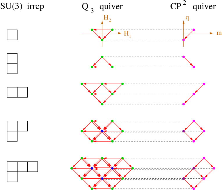
Figure 1: SU(3) irreps, weights and quiver diagrams

9 Nonabelian coupled vortex equations

The condition of $G$-equivariance together with the data $\{{\mathcal{D}},k_{i}\}$ uniquely determine the dependence of ${\mathcal{A}}$ and ${\mathcal{F}}$ on the coset coordinates. Therefore, the Yang-Mills and DUY equations dimensionally reduce to equations for $A^{i}$ (or $F^{i}$) $\in u(k_{i})$ and $\phi_{ij}\in\text{Hom}({\mathbb{C}}^{k_{j}},{\mathbb{C}}^{k_{i}})$ on ${\mathcal{M}}_{2n}$ only, with the indices $i,j=0,1,\ldots,m$ running over the vertices of the quiver and index pairs $(i,j)$ labelling the blocks in (10). For explicitness, we introduce local holomorphic coordinates $\{z^{a}\}$ with $a=1,2,\dots,n$ on ${\mathcal{M}}_{2n}$, so that the $\mathrm{U}(k_{i})$ connection and field strength take the form

$$A^{i}\ =\ A^{i}_{a}\,\mathrm{d}z^{a}+A^{i}_{\bar{a}}\,\mathrm{d}{\bar{z}}^{\bar{a}}\qquad\longrightarrow\qquad F^{i}\ =\ F^{i}_{ab}\,\mathrm{d}z^{a}{\wedge}\mathrm{d}z^{b}+2F^{i}_{a{\bar{b}}}\,\mathrm{d}z^{a}{\wedge}\mathrm{d}{\bar{z}}^{\bar{b}}+F^{i}_{{\bar{a}}{\bar{b}}}\,\mathrm{d}{\bar{z}}^{\bar{a}}{\wedge}\mathrm{d}{\bar{z}}^{\bar{b}}$$ (22)

with  $(A^{i}_{a})^{\dagger}=-A^{i}_{\bar{a}}$  and  $(F^{i}_{ab})^{\dagger}=F^{i}_{{\bar{a}}{\bar{b}}}$,  $(F^{i}_{a{\bar{b}}})^{\dagger}=F^{i}_{{\bar{a}}b}$  etc.. For the rank-one case with  ${\mathcal{D}}=\underline{$m{+}1$}$  and redenoting  $\phi_{ij}=:\phi_{i,j}$, the DUY equations on  ${\mathcal{M}}_{2n}\times{\mathbb{C}}P^{1}$  descend to

$$F^{i}_{ab}\ =\ 0\ =\ F^{i}_{{\bar{a}}{\bar{b}}}\quad,\qquad D_{\bar{a}}\,\phi_{i,i+1}\ =\ 0\ =\ D_{a}\,\phi_{i+1,i}\quad,$$ (23)

$$g^{a{\bar{b}}}\,F^{i}_{a{\bar{b}}}\ =\ {\textstyle\frac{1}{2R^{2}}}\bigl{(}{m{-}2i}\ +\ \phi_{i,i-1}\phi_{i-1,i}\ -\ \phi_{i,i+1}\phi_{i+1,i}\bigr{)}\ ,$$ (24)

where $D$ denotes the gauge covariant derivative, and $\phi_{0}=\phi_{m+1}=0$. We call this set of relations the “nonabelian chain vortex equations” with data $({\mathcal{M}}_{2n},R,m,\{k_{i}\})$.

10 Seiberg-Witten monopole equations

The simplest nontrivial case occurs for  ${\mathcal{M}}_{4}$ (i.e. $n{=}2$), a spin-$\frac{1}{2}$ representation (i.e. $m{=}1$) and the breaking $\mathrm{U}(2)\to\mathrm{U}(1)\times\mathrm{U}(1)$. Dropping irrelevant indices, $\boldsymbol{1}$s and $\otimes$s, the connection becomes

$${\mathcal{A}}\ =\ \begin{pmatrix}A^{0}(z)+a_{+1}(y)&\phi(z)\,\bar{\beta}(y)\\[24.0pt] -\bar{\phi}(z)\,\beta(y)&A^{1}(z)+a_{-1}(y)\end{pmatrix}\ .$$ (25)

The DUY equations then imply  $A^{0}=-A^{1}=:A$  and simplify to

$$F_{ab}\ =\ 0\ =\ F_{{\bar{a}}{\bar{b}}}\quad,\qquad\partial_{\bar{a}}\,\phi+2A_{\bar{a}}\,\phi\ =\ 0\quad,\qquad g^{a{\bar{b}}}\,F_{a{\bar{b}}}\ =\ {\textstyle\frac{1}{2R^{2}}}\bigl{(}1-\phi\,\bar{\phi}\bigr{)}\ ,$$ (26)

which are known as the “perturbed abelian Seiberg-Witten monopole equations”.[16] On ${\mathcal{M}}_{4}={\mathbb{R}}^{4}$, the latter admit only trivial solutions; one of the reasons why we shall now apply a noncommutative deformation.[17]

11 Moyal deformation

For the remainder of the talk we specialize to  ${\mathcal{M}}_{2n}={\mathbb{C}}^{n}$  in order to Moyal deform the base manifold. This deformation is realized by the Moyal-Weyl map sending

Schwartz functions $$f \qquad\longmapsto\qquad \widehat{f}$$ compact operators (27)

coordinates $$z^{a} \bar{z}^{\bar{b}} \qquad\longmapsto\qquad \widehat{z}^{a} \widehat{\bar{z}}\vphantom{z}^{\bar{b}}$$ and operators and (28)

subject to  $[\widehat{z}^{a},\widehat{\bar{z}}\vphantom{z}^{\bar{b}}]=\theta^{a{\bar{b}}}$  with an antisymmetric matrix $(\theta^{a{\bar{b}}})$. We can always rotate the coordinates such that

$$\theta^{a{\bar{b}}}\ =\ 2\delta^{ab}\,\theta^{a}\qquad\text{for}\quad\theta^{a}\in{\mathbb{R}}_{+}\quad\text{with}\quad a,b=1,\dots,n\ .$$ (29)

This defines the noncommutative space  ${\mathbb{C}}^{n}_{\theta}$, with isometry $\mathrm{USp}(n)$ and carrying $n$ copies of the Heisenberg algebra,

$$\bigl{[}{\textstyle\frac{\widehat{z}^{a}}{\sqrt{2\theta^{a}}}}\,,\,{\textstyle\frac{\widehat{\bar{z}}\vphantom{z}^{\bar{b}}}{\sqrt{2\smash{\theta^{b}}}}}\bigr{]}\ =\ \delta^{ab}\ .$$ (30)

To represent this algebra, we need to introduce an auxiliary Fock space ${\mathcal{H}}$. Finally, we remark that derivatives and integrals are represented as follows ($\theta^{a{\bar{b}}}\,\theta_{{\bar{b}}c}=\delta^{a}_{c}$),

$$\partial_{\bar{b}}f\ \longmapsto\ \theta_{{\bar{b}}c}\,[\widehat{z}^{c},\widehat{f}]\qquad\text{and}\qquad\smallint\!\mathrm{d}\mathrm{V}\,f\ \longmapsto\ (2\pi)^{n}\mathrm{Pf}(\theta)\,\mathrm{tr}_{\mathcal{H}}\widehat{f}\ .$$ (31)

12 Noncommutative chain vortex system

How do the nonabelian chain vortex equations (23, 24) change under the Moyal deformation? Dropping the hats from now on, we define “covariant coordinates”

$$X^{i}_{a}\ :=\ A^{i}_{a}\ +\ \theta_{a{\bar{b}}}\,{\bar{z}}^{\bar{b}}\qquad\text{and}\qquad X^{i}_{\bar{a}}\ :=\ A^{i}_{\bar{a}}\ +\ \theta_{{\bar{a}}b}\,z^{b}$$ (32)

and express the field strengths and Higgs gradients through them,

$$F^{i}_{ab}\ =\ [X^{i}_{a},X^{i}_{b}]\ ,\quad F^{i}_{a{\bar{b}}}\ =\ [X^{i}_{a},X^{i}_{\bar{b}}]\ +\ \theta_{a{\bar{b}}}\quad\text{and}\quad D_{\bar{a}}\,\phi_{i,i+1}\ =\ X^{i}_{\bar{a}}\,\phi_{i,i+1}-\phi_{i,i+1}X^{i+1}_{\bar{a}}\ .$$ (33)

With this, the DUY/vortex equations (23, 24) reduce to algebraic equations for $\{X^{i},\phi_{i,i+1}\}$:

$$[X^{i}_{a},X^{i}_{b}]\ =\ 0\ =\ [X^{i}_{\bar{a}},X^{i}_{\bar{b}}]\quad,\qquad X^{i}_{\bar{a}}\,\phi_{i,i+1}\ -\ \phi_{i,i+1}X^{i+1}_{\bar{a}}\ =\ 0\quad,$$ (34)

$$\delta^{ab}\,\bigl{(}[X^{i}_{a},X^{i}_{\bar{b}}]+\theta_{a{\bar{b}}}\bigr{)}\ =\ {\textstyle\frac{1}{4R^{2}}}\bigl{(}m{-}2i\ +\ \phi_{i,i-1}\phi_{i-1,i}\ -\ \phi_{i,i+1}\phi_{i+1,i}\bigr{)}\ .$$ (35)

13 BPS solutions

We remain with the $\frac{G}{H}={\mathbb{C}}P^{1}$ case and consider momentarily the particular situation of $k_{1}=\ldots=k_{m}=:r$, i.e. gauge group  $\mathrm{U}(k_{0})\times\mathrm{U}(r)^{m}$. In this context, a good ansatz is

$$A^{i}_{a}\ =\ 0\qquad\text{and}\qquad\phi_{i,i+1}\sim\ \boldsymbol{1}_{r}\qquad\text{for}\quad i=1,2,\dots,m$$ (36)

but $$A^{0}_{a}\ =\ \theta_{a{\bar{b}}}\,\bigl{(}T\,{\bar{z}}^{b}\,T^{\dagger}\ -\ {\bar{z}}^{b}\bigr{)}\qquad\text{and}\qquad\phi_{0,1}\ =\ \sqrt{m}\;T\ ,$$ (37)

with a partial isometry realized by a $k_{0}{\times}r$ matrix $T$ (Toeplitz operator) obeying

$$T^{\dagger}T\ =\ \boldsymbol{1}_{r}\ ,\qquad T\,T^{\dagger}\ =\ \boldsymbol{1}_{k_{0}}-P\ ,\qquad P^{2}=P=P^{\dagger}\quad\text{with}\quad\text{rk}(P)=:N\ .$$ (38)

Suitable operators $T$ obtain from an $\mathrm{SU}(2)$-equivariant generalization of the ABS construction [18]. With this ansatz, the field strengths and Higgs gradients become

$$F^{i}_{\cdot\cdot}=0\qquad\text{except}\qquad F^{0}_{a{\bar{b}}}=\theta_{a{\bar{b}}}\,P\qquad\text{and}\qquad D_{\bar{a}}\,\phi_{i,i+1}=0=D_{a}\,\phi_{i,i+1}\ .$$ (39)

Finally, plugging the ansatz into the noncommutative chain vortex system (34, 35), we observe that all equations are fulfilled provided

$$\sum_{a=1}^{n}\frac{1}{\theta^{a}}\ =\ \frac{m}{2R^{2}}\ ,$$ (40)

a nontrivial relation between the deformation strength and the size of the coset space!

14 Non-BPS solutions

Turning on more than one quiver vertex in the ansatz above fails to produce a nontrivial solution to the noncommutative DUY/vortex equations. Nevertheless, let us consider the general situation of $\prod_{i}\mathrm{U}(k_{i})$ as the gauge group and generalize the ansatz (36, 37) to

$$A^{i}_{a}\ =\ \theta_{a{\bar{b}}}\,\bigl{(}T_{i}^{\phantom{\dagger}}{\bar{z}}^{b}\,T_{i}^{\dagger}-{\bar{z}}^{b}\bigr{)}\qquad\text{and}\qquad\phi_{i,i+1}\ =\ \alpha_{i+1}\,T_{i}^{\phantom{\dagger}}\,T_{i+1}^{\dagger}\quad\text{with}\quad\alpha_{i}\in{\mathbb{C}}\ ,$$ (41)

where $m{+}1$ partial isometries are realized by $k_{i}{\times}r$ matrices $T_{i}$ (Toeplitz operators):

$$T_{i}^{\dagger}T_{i}^{\phantom{\dagger}}\ =\ \boldsymbol{1}_{r}\ ,\qquad T_{i}^{\phantom{\dagger}}T_{i}^{\dagger}\ =\ \boldsymbol{1}_{k_{i}}-P_{i}^{\phantom{\dagger}}\ ,\qquad P_{i}^{2}=P_{i}^{\phantom{\dagger}}=P_{i}^{\dagger}\quad\text{of rank}\ N_{i}\ .$$ (42)

This ansatz implies

$$F^{i}_{ab}\ =\ 0\ =\ F^{i}_{{\bar{a}}{\bar{b}}}\ ,\quad F^{i}_{a{\bar{b}}}\ =\ \theta_{a{\bar{b}}}\,P_{i}\ ,\quad D_{\bar{a}}\,\phi_{i,i+1}\ =\ 0\ =\ D_{a}\,\phi_{i,i+1}$$ (43)

$$\text{and}\qquad|\alpha_{i}|^{-2}\,\phi_{i,i-1}\,\phi_{i-1,i}\ =\ \boldsymbol{1}_{k_{i}}-P_{i}\ =\ |\alpha_{i+1}|^{-2}\,\phi_{i,i+1}\,\phi_{i+1,i}\ ,$$ (44)

which finally contradicts (35) if more than one projector is nonzero.

Surprisingly, however, it does solve the full noncommutative Yang-Mills equations! The energy of the so-constructed non-BPS configurations is given by

$$E\ =\ 2\pi R^{2}\bigl{(}\prod_{a=1}^{n}2\pi\theta^{a}\bigr{)}\sum_{i=0}^{m}\,\text{Tr}_{\mathcal{H}}\,\bigl{[}\lambda_{i}\,P_{i}\ +\ \mu_{i}\,(\boldsymbol{1}_{k_{i}}{-}P_{i})\bigr{]}$$ (45)

$$\text{with}\qquad\textstyle\lambda_{i}\ =\ \sum_{b}\frac{1}{(\theta^{b})^{2}}\ +\ \frac{(m{-}2i)^{2}}{4\,R^{4}}\qquad\text{and}\qquad\mu_{i}\ =\ \frac{(m{-}2i{+}|\alpha_{i}|^{2}{-}|\alpha_{i+1}|^{2})^{2}}{4\,R^{4}}\ ,$$ (46)

where $\alpha_{0}=\alpha_{m+1}=0$. Finite energy requires $\mu_{i}=0$ for $i=0,1,\ldots,m$, which determines $|\alpha_{i+1}|^{2}=(i{+}1)(m{-}1)$. The BPS solution (39) with (40) is seen as a special case: Putting $P_{1}=\ldots=P_{m}=0$ (and $\mu_{i}=0$) yields

$$E_{\text{BPS}}\ =\ 2\pi R^{2}\bigl{(}\prod_{a=1}^{n}2\pi\theta^{a}\bigr{)}\,\lambda_{0}\,\text{Tr}_{\mathcal{H}}\,P_{0}\qquad\text{with}\qquad\lambda_{0}\ =\ 2\sum_{b\leq c}(\theta^{b}\theta^{c})^{-1}\ .$$ (47)

15 D-brane interpretation

Our construction and the constructed classical field configurations allow for a D-brane interpretation. For simplicity, let us stay with the $\frac{G}{H}={\mathbb{C}}P^{1}$ case. One has a higher-dimensional and a lower-dimensional picture:

“Upstairs” on ${\mathbb{C}}^{n}_{\theta}\times S^{2}$ we began with $k$ coincident D($2n{+}2$)-branes wrapping the $S^{2}$. The $\mathrm{SU}(2)$-equivariance condition splits $k\to\{k_{i}\}$ and wraps the $S^{2}$ with charge-$q_{i}$ monopole fields, for $i=0,\ldots,m$.

“Downstairs” on ${\mathbb{C}}^{n}_{\theta}$ we find $m{+}1$ subsets of D($2n$)-branes carrying magnetic fluxes $q_{i}$. On each subset of these space-filling branes live Chan-Paton gauge fields $A^{i}\in\mathrm{End}(E_{k_{i}})$, and neighboring subsets are connected by Higgs fields $\phi_{i,i+1}\in\mathrm{Hom}(E_{k_{i+1}},E_{k_{i}})$ which correspond to massless open-string excitations.

This chain of brane subsets is marginally bound but stabilized by the magnetic fluxes. The BPS vortex configurations we have constructed are bound states of $mN$ D0-branes inside the D($2n$)-brane system. The energy and topological charge of such a BPS state is most elegantly computed via equivariant K-homology.

The aforesaid generalizes to quivers based on higher-rank Lie groups and their corresponding vortex-type equations, but some new features will arise due to nontrivial Higgs-field relations and quiver vertex degeneracies.

References

- [1] D. Kapetanakis and G. Zoupanos, \PRP219,1992,1.
- [2] E. Witten, \PRL38,1977,121.
- [3] P. Forgacs and N. S. Manton, \CMP72,1980,15.
- [4] N. S. Manton, \NPB193,1981,502.
- [5] P. Manousselis and G. Zoupanos, \PLB504,2001,122 [hep-ph/0010141].
-
[6]
G. Lopes Cardoso, G. Curio, G. Dall’Agata, D. Lüst, P. Manousselis and
G. Zoupanos, \NPB652,2003,5 [hep-th/0211118]. - [7] O. García-Prada, \CMP156,1993,527; \JLInt. J. Math.,5,1994,1.
-
[8]
L. Álvarez-Cónsul and O. García-Prada,
\JLInt. J. Math.,12,2001,159
[math.dg/0112159]. -
[9]
L. Álvarez-Cónsul and O. García-Prada,
\JLJ. Reine Angew. Math.,556,2003,1
[math.dg/0112160]. -
[10]
L. Álvarez-Cónsul and O. García-Prada,
\CMP238,2003,1
[math.dg/0112161]. -
[11]
O. Lechtenfeld, A. D. Popov and R. J. Szabo,
\JHEP0312,2003,022 [hep-th/0310267]. - [12] A. D. Popov and R. J. Szabo, \JMP47,2006,012306 [hep-th/0504025].
-
[13]
O. Lechtenfeld, A. D. Popov and R. J. Szabo,
\JHEP0609,2006,054 [hep-th/0603232]. -
[14]
S. K. Donaldson,
\JLProc. Lond. Math. Soc.,50,1985,1;
\JLDuke Math. J.,54,1987,231. -
[15]
K. K. Uhlenbeck and S.-T. Yau,
\JLCommun. Pure Appl. Math.,39,1986,257;
ibid. \andvol42,1989,703. - [16] E. Witten, \JLMath. Res. Lett.,1,1994,769 [hep-th/9411102].
-
[17]
A. D. Popov, A. G. Sergeev and M. Wolf,
\JMP44,2003,4527
[hep-th/0304263]. - [18] M. F. Atiyah, R. Bott and A. Shapiro, \JLTopology,3,1964,3.