Analytical approximation schemes for solving exact renormalization group equations in the local potential approximation

Abstract

The relation between the Wilson-Polchinski and the Litim optimized ERGEs in the local potential approximation is studied with high accuracy using two different analytical approaches based on a field expansion: a recently proposed genuine analytical approximation scheme to two-point boundary value problems of ordinary differential equations, and a new one based on approximating the solution by generalized hypergeometric functions. A comparison with the numerical results obtained with the shooting method is made. A similar accuracy is reached in each case. Both two methods appear to be more efficient than the usual field expansions frequently used in the current studies of ERGEs (in particular for the Wilson-Polchinski case in the study of which they fail).

,,

1 Introduction

The non-decoupling of the relevant scales on a wide and continuous range of magnitudes in many areas of physics has led to the invention (discovery) of the renormalisation group (RG) [1]. Whereas they have been discovered in the framework of the perturbative (quantum field) theory, the RG techniques tackle a nonperturbative physical phenomenon [2]. Nonperturbative approaches are difficult to implement and to control, and during a long time one has essentially carried on perturbative RG techniques (see, e.g., [3]). Nowadays, the huge growth of the computing capacity has greatly modified this behaviour pattern and, already since the beginning of the ninety’s, one has considered [4] with a greater acuteness the exact RG equations (ERGEs) originally introduced by Wilson [5], Wegner and Houghton [6] in the seventy’s and slightly reformulated by Polchinski [7] in the eighty’s (for some reviews on the ERGEs see [8]).

Initially, the ERGEs are integro-differential equations for the running action $S\left[\phi,t\right]$ [assuming that $\phi\left(x\right)$ generically stands for some field with as many indices as necessary and $t=-\ln\left(\Lambda/\Lambda_{0}\right)$ the logarithm of a running momentum scale $\Lambda$]. They have been extended to the running (average) effective action $\Gamma\left[\varphi,t\right]$ [9, 4]. Such general equations cannot be studied without the recourse to approximations or truncations. One of the most promising approximations is a systematic expansion in powers of the derivative of the field (derivative expansion) [10] which yields a set of coupled nonlinear partial differential equations the number of which grows quickly with the order of the expansion. In the simplest cases (e.g., for the scalar field), the determination of fixed points (and of their stability) amounts to study ordinary differential equations (ODEs) with a two-point boundary value problem that may be carried out numerically via a shooting (or a relaxation) method.

A pure numerical study is in general not easy to implement and to control. For example, in the shooting method, the discovery of the right adjustment of the parameters at the boundaries requires a good knowledge a priori of their orders of magnitude (initial guesses). It is thus interesting to develop concurrently some substitute analytical methods. A popular substitute to the ODEs of the derivative expansion is provided by an additionnal expansion in powers of the field which yields a set of coupled algebraic equations which may be solved analytically, at least with the help of a symbolic computation software. Various field expansions have been implemented with more or less success [11, 12, 13, 14]. Unfortunately, the methods proposed up to now, if they are easy to implement, do not work in all cases and especially in the most famous and simplest case of the Wilson-Polchinski ERGE [5, 7] (equation for the running action $S\left[\phi,t\right]$ with a smooth cutoff).

The object of this paper is to present two new substitute analytical methods for studying ODEs which, at least in the local potential approximation of the derivative expansion (LPA), works for the Wilson-Polchinski ERGE. One of the methods, recently proposed in [15], is a genuine analytical approximation scheme to two-point boundary value problems of ODEs. The other method is new. It is based on approximations of the solution looked for by generalized hypergeometric functions. It has a certain similarity with another new and interesting method based on the representation of the solution by Padé approximants just proposed in [16] by P. Amore and F. M. Fernandez independantly from the present work. We illustrate the effectiveness of the two methods with the explicit consideration of two ERGEs in the local potential approximation: the Wilson-Polchinski equation and the Litim optimized RG equation [17] for the running effective action (named the Litim equation in the following). Following a conjecture first stated in [18, 19], the equivalence of these two equations (in the LPA) has been proven by Morris [20] and recently been numerically illustrated [21] with an unprecedented accuracy for the scalar field in three dimensions ($d=3$). This particular situation provides us with the opportunity of testing efficiently the various methods of study at hand.

The following of the paper is divided in five sections. In section 2, we briefly present the direct numerical integration of the ODEs for the scalar model using the shooting method: determinations of the fixed point and the critical exponents for both the Wilson-Polchinski and Litim equations in the LPA (distinguishing between the even and odd symmetries). A brief presentation of the currently used field expansion is given in section 3. In section 4, we analyse several aspects of the method of [15] applying it to the study of the two equations. We calculate this way the fixed point locations with high precision and compare the results with the estimates obtained in section 2. We show how the leading and the subleading critical exponents may be estimated using this recent method. In section 5 we present a new approximate analytical method for ODEs which is based on the definition of the generalized hypergeometric functions. We show that it is well adapted to treat the Wilson-Polchinski case whereas the Litim case is less easily treated. We relate these effects to the convergence properties of the series in powers of the field. Finally we summarize this work and conclude in section 6.

2 Two-point boundary value problem in the LPA

In this section we briefly present the two-point boundary value problem to be solved in the LPA of the ERGE. The Wilson-Polchinski equation is first chosen as a paradigm in section 2.1. The principal numerical results obtained from the numerical integration of the ODE using the shooting method are given. In section (2.2), the Litim equation is also studied.

2.1 Wilson-Polchinski’s flow equation for the scalar-field

The original Wilson-Polchinski ERGE in the LPA expresses the evolution of the potential $U\left(\phi,t\right)$ as varying the logarithm of the momentum scale of reference $t=-\ln\left(\Lambda/\Lambda_{0}\right)$ (with $\phi\in\mathbb{R}$). In three dimensions, it reads:

$$\dot{U}=U^{\prime\prime}-\left(U^{\prime}\right)^{2}-\frac{1}{2}\phi U^{\prime}+3U\,,$$ (1)

in which $\dot{U}\equiv\partial U\left(\phi,t\right)/\partial t$, $U^{\prime}\equiv\partial U\left(\phi,t\right)/\partial\phi$, $U^{\prime\prime}\equiv\partial^{2}U\left(\phi,t\right)/\partial\phi^{2}$.

2.1.1 Fixed point equation

The fixed point equation corresponds to $\dot{U}=0$. It is a second order ODE for the function $U\left(\phi\right)$:

$$U^{\prime\prime}-\left(U^{\prime}\right)^{2}-\frac{1}{2}\phi U^{\prime}+3U=0\,,$$ (2)

the solution of which (denoted $U^{\ast}\left(\phi\right)$ below) depends on two integration constants which are fixed by two conditions. The first one comes from a property of symmetry assumed to be $U^{\ast}\left(-\phi\right)=U^{\ast}\left(\phi\right)$ which provides the following condition at the origin for $U^{\ast}\left(\phi\right)$:

$$U^{\ast\prime}\left(0\right)=0\,.$$ (3)

The second condition is the requirement that the solution we are interested in must be non singular in the entire range $\phi\in\left[0,\infty\right[$. Actually, the general solution of (2) involves a moving singularity [22] of the form:

$$U_{\text{sing}}=-\ln\left|\phi_{0}-\phi\right|\,,$$ (4)

depending on the arbitrary constant $\phi_{0}$. Pushing $\phi_{0}$ to infinity allows to get a non-singular potential since, in addition to the two trivial fixed points $U^{\ast}\equiv 0$ (Gaussian fixed point) and $U^{\ast}\equiv-\frac{1}{3}+\frac{{\phi}^{2}}{2}$ (high temperature fixed point), eq.(2) admits a non-singular solution which, for $\phi\rightarrow\infty$, has the form:

$$U_{\text{asy}}(\phi)=\frac{{\phi}^{2}}{2}+b\,{\phi}^{\frac{6}{5}}+\frac{18\,b^{2}\,{\phi}^{\frac{2}{5}}}{25}-\frac{1}{3}+\frac{108\,b^{3}}{625\,{\phi}^{\frac{2}{5}}}+O\left(\phi^{-4/5}\right)\,,$$ (5)

in which $b$ is the only remaining arbitrary integration constant. The non trivial (Wilson-Fisher [23]) fixed point solution which we are interested in must interpolate between eqs. (3) and (5). Imposing these conditions fixes uniquely the value $b^{\ast}$ of $b$ which corresponds to the fixed point solution we are looking for.

We have determined $b^{\ast}$ by using the shooting method [24]: starting from a value $\phi_{a}$ supposed to be large where the condition (5) is imposed (with a guess, or trying, value of $b\simeq b^{\ast}$), we integrate the differential equation (2) toward the origin where the condition (3) is checked (shooting to the origin), we adjust the value of $b$ to $b^{\ast}$ so as the latter condition is satisfied with a required accuracy. A study of the stability of the estimate of $b^{\ast}$ so obtained on varying the value $\phi_{a}$ provides some information on the accuracy of the calculation.

Rather than (5), it is more usual to characterize the fixed point solution from its small field behaviour:

$$U(\phi)=k-\frac{3\,k\,}{2}\phi^{2}+\frac{k\,\left(1+3\,k\right)\,}{4}\phi^{4}-\frac{k\,\left(1+3\,k\right)\,\left(1+24\,k\right)\,}{120}\phi^{6}+O\left(\phi^{8}\right)\,,$$ (6)

and to provide the value of either of the two (related) quantities:

$$k^{\ast} = U^{\ast}\left(0\right)\,,$$ (7)

$$r^{\ast} = U^{\ast\prime\prime}\left(0\right)=-3k^{\ast}\,.$$ (8)

In the shooting-to-origin method, the determination of $r^{\ast}$ (or $k^{\ast}$) is a byproduct of the adjustment of $b^{\ast}$.

The adjustment of $b^{\ast}$ may be bypassed by shooting from the origin toward $\phi_{a}$, then $r^{\ast}$ is adjusted in such a way as to reach the largest possible value of $\phi_{a}$. In that case $b^{\ast}$ is a byproduct of the adjustment.

Because the boundary condition at $\phi_{a}$ is under control, the shooting-to-origin method provides a better determination of $r^{\ast}$ than the shooting-from-origin method. However, this latter method is more flexible and may easily yield a rough estimate on $r^{\ast}$ which can be used as a guess in a more demanding management of the method. Notice that, due to the increase of the number of adjustable parameters, this way of determining a guess is no longer possible in a study involving several coupled EDOs. Consequently, the development of other methods as, for example, those two presented below is useful to this purpose (see also [16]).

$r^{\ast}$		$b^{\ast}$		$\phi_{a}$
$-0.228\,598\,202\,437\,022\,0$		$\allowbreak-2.\,\allowbreak 296\,3$		$10$
$-0.228\,598\,202\,437\,021\,9$		$\allowbreak-2.\,\allowbreak 311\,6$		$20$
$-0.228\,598\,202\,437\,021\,9$		$\allowbreak-2.\,\allowbreak 316\,2$		$40$

Table 1: The fixed point parameter $r^{\ast}$ is already well determined for rather small values of $\phi_{a}$ whereas $b^{\ast}$ [fixed point value of $b$ in (5)] still is not.

Table 1 displays the determinations of $r^{\ast}$ and $b^{\ast}$ for three values of $\phi_{a}$. One may observe that a high accuracy on $r^{\ast}$ is required to reach a yet small value of $\phi_{a}$ whereas $b^{\ast}$ is only poorly determined. Obviously, considering higher values of $\phi_{a}$ and/or higher order terms in eq. (5) allows to better determine $b^{\ast}$, one more term in (5) and $\phi_{a}=1000$ yields:

$$b^{\ast}=-2.318\,29\,,$$ (9)

but the estimate of $r^{\ast}$ is not improved compared to the values given in table 1 (the machine-precision was already reached). We finally extract from table 1 our best estimate of $r^{\ast}$ (or $k^{\ast}$) as obtained from the study of the fixed point equation (2) alone:

$$r^{\ast} = -0.228\,598\,202\,437\,022\pm 10^{-15}\,\,,$$ (10)

$$k^{\ast} = 0.076\,199\,400\,812\,340\,7\pm 10^{-16}\,.$$ (11)

Individually, these values do not define the potential function $U^{\ast}\left(\phi\right)$ the knowledge of which requires the numerical integration explicitly performed in the shooting method.

2.1.2 Eigenvalue equation

The critical exponents are obtained by linearizing the flow equation (1) near the fixed point solution $U^{\ast}\left(\phi\right)$. If one inserts:

$$U\left(\phi,t\right)=U^{\ast}\left(\phi\right)+\epsilon\,e^{\lambda t}g\left(\phi\right)\,,$$

into the flow equation and keeps the linear terms in $\epsilon$, one obtains the eigenvalue equation:

$$g^{\prime\prime}-2\,g^{\prime}U^{\ast\prime}-\frac{\phi}{2}\,g^{\prime}+\left(3-\lambda\right)\,g=0\,.$$ (12)

Again it is a second order ODE the solutions of which are characterized by two integration constants.

Since $U^{\ast}\left(\phi\right)$ is an even function of $\phi$, eq. (12) is invariant under a parity change. Then one of the integration constants is fixed by looking for either an even or an odd eigenfunction $g\left(\phi\right)$ which implies either $g^{\prime}\left(0\right)=0$ (even) or $g\left(0\right)=0$ (odd). The second integration constant is fixed at will due to the arbitrariness of the normalisation of an eigenfunction. Thus, assuming either $g\left(0\right)=1$ (even) or $g^{\prime}\left(0\right)=1$ (odd), the solutions of (12) depend only on $\lambda$ and on the fixed point parameter $k^{\ast}$. For example, these solutions have the following expansions about the origin $\phi=0$ :

$$g_{\text{even}}\left(\phi\right)=1+\frac{\left(\lambda-3\right)}{2}\phi^{2}\left[1+\frac{\,\,\left(\lambda-2-12\,k^{\ast}\right)}{12}\phi^{2}\right]+O\left(\phi^{6}\right)\,,$$

$$g_{\text{odd}}\left(\phi\right)=\phi+\frac{\,\left(2\,\lambda-5-12\,k^{\ast}\right)}{12}\phi^{3}+O\left(\phi^{5}\right)\,.$$

When the fixed point solution $U^{\ast}$ is known, the values of $\lambda$ [the only remaining unknown parameter in (12)] are determined by looking for the solutions which interpolate between either $g^{\prime}\left(0\right)=0$ (even) or $g\left(0\right)=0$ (odd) and the regular solution of (12)

which, for $\phi\rightarrow\infty$, is:

$$g_{\text{asy}}(\phi)=S_{0}{\phi}^{\frac{2\,\left(3-\lambda\right)}{5}}\left\{1+\left(3-\lambda\right)\left[\frac{12\,b^{\ast}\,}{25\,{\phi}^{\frac{4}{5}}}-\frac{36\,b^{\ast 2}\,\left(2\,\lambda-3\right)}{625\,{\phi}^{\frac{8}{5}}}+\frac{2\,\,\left(2\,\lambda-1\right)}{125\,{\phi}^{2}}+O\left({\phi}^{-\frac{12}{5}}\right)\right]\right\}\,,$$ (13)

in which $b^{\ast}$ is given by (9). The value of $S_{0}$ is related to the choice of the normalisation of the eigenfunction at the origin, it is a byproduct of the adjustment in a shooting-from-origin procedure.

In the even case, it is known that the first nontrivial positive eigenvalue $\lambda_{1}$ (there is also the trivial value $\lambda_{0}=d=3$), is related to the critical exponent $\nu$ which characterizes the Ising-like critical scaling of the correlation length $\xi$. One has $\nu=1/\lambda_{1}$ and the first negative eigenvalue, $\lambda_{2}$, is minus the Ising-like first correction-to-scaling exponent $\omega_{1}$ ($\omega_{1}=-\lambda_{2}$) and so on.

In the odd case, the two first (positive) eigenvalues are trivial in the LPA. One has:

$$\breve{\lambda}_{1} = \frac{d+2-\eta}{2}\,,$$ (14)

$$\breve{\lambda}_{2} = \frac{d-2+\eta}{2}\,,$$ (15)

in which $\eta$ is the critical exponent which governs the large distance behaviour of the correlation functions right at the critical point, it vanishes in the LPA. With the dimension $d=3$ and the approximation (LPA) presently considered, (14) and (15) reduce to $\breve{\lambda}_{1}=2.5$ and $\breve{\lambda}_{2}=0.5$. Consequently the first non-trivial eigenvalue is negative and defines the subcritical exponent $\theta_{5}=\breve{\omega}_{1}=-\breve{\lambda}_{3}$ sometimes considered to characterize the deviation of the critical behaviour of fluids from the pure Ising-like critical behaviour.

$\nu$		$b^{\ast}$		$\phi_{a}$
$0.649\,561\,773\,880\,11$		$-2.\,\allowbreak 318\,145$		$12$
$0.649\,561\,773\,880\,80$		$-2.318\,257$		$22$
$0.649\,561\,773\,880\,65$		$-2.318\,280$		$32$
$0.649\,561\,773\,880\,65$		$-2.318\,285$		$40$

Table 2: Values of the critical exponent $\nu$ determined together with $b^{\ast}$ (and thus $r^{\ast}$) whereas $\phi_{a}$ is varied. Compared to table 1, a better determination of $b^{\ast}$ is obtained [see the best value of $b^{\ast}$  given by eq. (9)].

To determine the eigenvalues we use again the shooting-to-origin method with the two equations (2, 12). However, in addition to $\lambda$, we leave also $b^{\ast}$ adjustable instead of fixing it to the value given in (9).

In the even case, the values we obtain for $\nu$ and $b^{\ast}$ are shown in table 2 for four values of $\phi_{a}$. Comparing with the values displayed in table 1 one observes a better convergence of $b^{\ast}$ to the best value (9) whereas $r^{\ast}$ remains unchanged compared to (10). As for the best estimate of $\nu$, it is:

$$\nu_{\mathrm{best}}=0.649\,561\,773\,880\pm 10^{-12}\,,$$ (16)

that is to say:

$$\lambda_{1\mathrm{best}}=1.539\,499\,459\,808\pm 10^{-12}\,.$$ (17)

We have proceeded similarly to determine the Ising-like subcritical exponent values displayed in table 3.

$\omega_{1}$		$\omega_{2}$		$\omega_{3}$		$\omega_{4}$		$\omega_{5}$		$\omega_{6}$
$0.655\,745\,939\,193$		$3.180\,006\,512\,059$		$5.912\,230\,612$		$8.796\,092\,825$		$11.798\,087\,66$		$14.896\,053\,176$

Table 3: Best estimates of the six first subcritical exponents for the Ising-like scalar model (i.e. even case), all digits are significant.

In the odd case, we obtain:

$$\breve{\omega}_{1}=1.886\,703\,838\,091\pm 10^{-12}\,.$$ (18)

Table 4 displays the values of the other subcritical exponents of the same family as $\breve{\omega}$ but with a lower accuracy. Of course, the values presently obtained are in agreement with the previous estimates [25, 21].

$\breve{\omega}_{2}$		$\breve{\omega}_{3}$		$\breve{\omega}_{4}$
$4.524\,390\,734$		$7.337\,650\,643$		$10.283\,900\,73$

Table 4: Best estimates of the odd-case subcritical exponents other than $\breve{\omega}_{1}$ for the scalar model.

2.2 Litim’s flow equation for the scalar field

Following a conjecture first stated in [18, 19], the equivalence in the LPA between the Wilson-Polchinski flow (1) and the Litim optimized ERGE [17] for the running effective action $\Gamma\left[\varphi,t\right]$ has been proven by Morris [20]. The Litim flow equation for the potential $V\left(\varphi,t\right)$ reads in three dimensions (compared to [20] an unimportant shift $V\rightarrow V-1/3$ is performed):

$$\dot{V}=1-\frac{1}{1+V^{\prime\prime}}-\frac{\varphi}{2}V^{\prime}+3V\,.$$ (19)

It is related to (1) via the following Legendre transformation:

$$\left.\begin{array}[]{l}\left[\frac{1}{2}\phi^{2}-U\left(\phi,t\right)\right]+\left[\frac{1}{2}\varphi^{2}+V\left(\varphi,t\right)\right]=\varphi\phi\\ \varphi=\phi-U^{\prime}\left(\phi,t\right)\end{array}\right\}\,.$$ (20)

The general solution of the fixed point equation ($\dot{V}=0$) involves the following moving “singularity” ($V^{\prime\prime}$ is singular) at the arbitrary point $\varphi_{0}$:

$$V_{\text{sing}}\left(\varphi\right)=-\frac{1}{3}+\frac{4}{3\sqrt{\varphi_{0}}}\left|\varphi_{0}-\varphi\right|^{3/2}\,.$$ (21)

2.2.1 Fixed point solution

The numerical study of the fixed point solution of (19) follows the lines described in the preceding sections. This may be done independently, but due to (20), one may already deduce from the previous study the expected results. Similarly to (5), the asymptotic behaviour of the non trivial fixed point potential is characterized by the integration constant $b_{L}$ in the following expression [deduced from (19)]:

$$V_{\mathrm{asy}}(\varphi)=b_{L}\,{\varphi}^{6}-\frac{1}{3}+\frac{1}{150\,b_{L}\,{\varphi}^{4}}-\frac{1}{6300\,b_{L}^{2}\,{\varphi}^{8}}+O\left({\varphi}^{-12}\right)\,.$$ (22)

It is easy to show from (5) and (20) that the value $b_{L}^{\ast}$ we are looking for is related to $b^{\ast}$ as follows:

$$b_{L}^{\ast}\,=-\frac{1}{6^{6}}\left(\frac{5}{b^{\ast}}\right)^{5},$$

then, from the previous result (9) we get:

$$b_{L}^{\ast}\simeq 0.001\,000\,25\,.$$ (23)

Similarly for the potential parameters

$$k_{L}^{\ast} = V^{\ast}\left(0\right)\,,$$

$$r_{L}^{\ast} = V^{\ast\prime\prime}\left(0\right)\,,$$

which correspond to $b_{L}^{\ast}$, they are related to the Wilson-Polchinski counterparts $k^{\ast}$ and $r^{\ast}$ as follows:

$$k_{L}^{\ast} = k^{\ast}\,,$$ (24)

$$r_{L}^{\ast} = \frac{r^{\ast}}{1-r^{\ast}}\,.$$ (25)

This latter relation, using (10), gives:

$$r_{L}^{\ast}\simeq-0.186\,064\,249\,470\,314\pm 10^{-15}\,.$$ (26)

As precedingly, those values do not provide the potential function $V^{\ast}\left(\varphi\right)$ the knowledge of which requires an explicit numerical integration.

2.2.2 Eigenvalue equation

A linearization of the flow equation (19) near the fixed point solution $V^{\ast}\left(\varphi\right)$:

$$V\left(\varphi,t\right)=V^{\ast}\left(\varphi\right)+\epsilon\,e^{\lambda t}h\left(\varphi\right)\,,$$

provides the Litim eigenvalue equation:

$$\left(3-\lambda\right)\,h-\frac{\varphi\,h^{\prime}}{2}+\frac{h^{\prime\prime}}{{\left(1+{V^{\ast}}^{\prime\prime}\right)}^{2}}=0\,.$$ (27)

Taking into account (22), one can show that (27) admits a regular solution which, for $\varphi\rightarrow\infty$, has the form:

$$h_{\mathrm{asy}}\left(\varphi\right)=S_{1}{\varphi}^{2\,\left(3-\lambda\right)}\left\{1-\left(\lambda-3\right)\,\left(2\,\lambda-5\right)\left[\frac{1}{2250\,b_{L}^{\ast 2}\,{\varphi}^{10}}-\frac{1}{47250\,b_{L}^{\ast 3}\,{\varphi}^{14}}+O\left(\varphi^{-18}\right)\right]\right\}\,,$$ (28)

in which $b_{L}^{\ast}$ is given by (23). In the following we may set $S_{1}=1$ since the normalisation of the eigenfunction may be chosen at will.

As precedingly, we must distinguish between the odd and even eigenfunction $h\left(\varphi\right)$. The shooting method gives the same values as in the Wilson-Polchinski case (see [18, 26, 27, 21]) and we do not present them again.

3 Expansion in powers of the field

In advanced studies of the derivative expansion [28] or other efficient approximations of the ERGE [29] and in the consideration of complex systems via the ERGEs [30], a supplementary truncation in powers of the field is currently used (see also [8]). With a scalar field, this expansion transforms the partial differential flow equations into ODEs whereas the fixed point or eigenvalue ODEs are transformed into algebraic equations. Provided auxiliary conditions are chosen, the latter equations are easy to solve analytically using a symbolic computation software. Actually the auxiliary conditions currently chosen are extremely simple: they consist in setting equal to zero the highest terms of the expansion so as to get a balanced system of equations.

A first kind of expansion, about the zero field –referred to as the expansion I in the following, has been proposed by Margaritis et al [11] and applied to the LPA of Wegner-Houghton’s ERGE [6] (the hard cutoff version of the Wilson-Polchinski equation). A second kind of expansion, relative to the (running) minimum of the potential (expansion II), has been proposed by Tetradis and Wetterich [12] and more particularly presented by Alford [13] using it, again, with the sharp cutoff version of the ERGE.

It is known that, for the Wegner-Houghton equation in the LPA, expansion I does not converge due to the presence of singularities in the complex plane of the expansion variable [31]. Expansions I and II have been more concretely studied and compared to each other by Aoki et al in [14] who also propose a variant to II (expansion III) by letting the expansion point adjustable. They showed, again on the LPA of the Wegner-Houghton equation, that expansion II is much more efficient than expansion I although it finally does not converge and expansion III is the most efficient one. Expansions II and III work well also on the ERGE expressed on the running effective action (effective average action, see the review by Berges et al in [8]). The convergence of those expansions have also been studied in [26] according to the regularisation scheme chosen and in particular for the Litim equation (19). In this latter study it is concluded that both expansions I and II seem to converge although II converges faster than I.

A striking fact emerges from those studies, the Wilson-Polchinski equation in the LPA, the simplest equation, is never studied using the field expansion method. The reason is simple: none of the expansions currently used works in that case.

Actually the strategy of these methods, which consists in arbitrarily setting equal to zero one coefficient for the expansion I and two for the expansions II and III, is probably too simple. With regards to this kind of auxiliary conditions, the failure observed with the Wilson-Polchinski equation is not surprising and, most certainly, there should be many other circumstances where such simple auxiliary conditions would not solve correctly the derivative expansion of an ERGE.

In the following sections we examine two alternative methods with more sophisticated auxiliary conditions. We show that they yield the correct solution for the Wilson-Polchinski and its Legendre transformed (Litim) equations. Both methods are associated to expansion I (about the zero-field). The first one has recently been proposed in [15] as a method to treat the two point boundary value problem of ODEs. It relies upon an efficient account for the large field behaviour of the solution looked for. An attempt of accounting for this kind of behaviour within the field expansion had already been done by Tetradis and Wetterich via their eq. (7.11) of [12]. In the present work, a much more sophisticated procedure is used. It relies upon the construction of an added auxiliary differential equation (ADE). We refer to it in the following as the ADE method. The second method is new. It relies upon the approximation of the solution looked for by a generalized hypergeometric function. We refer to it in the following as the hypergeometric function approximation (HFA) method.

4 Auxiliary differential equation method

Let us first illustrate the auxiliary differential equation (ADE) method on the search for the non trivial fixed point in the LPA for both the Wilson-Polchinski equation (2) and the Litim optimized equation (19). Since there are two boundaries (the origin and the ”point at” infinity), we distinguish between two strategies.

• An expansion about the origin in the equations (small field expansion) and the account for the leading high field behaviour of the regular solution which we are looking for. This determines the value of $r^{\ast}$ or $r_{L}^{\ast}$.

• A change of variable $\phi\rightarrow 1/\phi$ or $\varphi\rightarrow 1/\varphi$ which reverses the problem: an expansion about infinity (new origin) in the equations (high field expansion) and the account for the leading small field behaviour of the regular solution which we are looking for. This determines the value of $b^{\ast}$ or $b_{L}^{\ast}$.

4.1 Wilson-Polchinski’s fixed point

4.1.1 Small field expansion and leading high field behaviour

For practical and custom reasons, instead of (2) we consider the equation satisfied by the function $w\left(x\right)$ related to the derivative of the potential $U^{\prime}\left(\phi\right)$ as follows:

$$U^{\prime}\left(\phi\right)=\phi\,w\left(\phi^{2}\right)\,,$$ (29)

so that, with $x=\phi^{2}$, the fixed point equation (2) reads:

$$4\,x\,w^{\prime\prime}-2\,{w}^{2}-4\,x\,w\,w^{\prime}+\left(6-\,x\right)\,\,w^{\prime}+2\,w=0\,,$$ (30)

in which a prime indicates a derivative with respect to $x$.

This second order ODE has a singular point at the origin and, by analyticity requirement, the solution we are looking for depends on a single unknown integration-constant (noted $r$ below).

Let us first introduce the expansion I of Margaritis et al [11]. The function $w\left(x\right)$ is expanded up to order $M$ in powers of $x$:

$$w_{M}\left(x\right)=r+\sum\limits_{n=1}^{M}a_{n}x^{n}\,,$$ (31)

and inserted into the fixed point equation (30).

Requiring that (30) be satisfied order by order in powers of $x$ provides an unbalanced system of $M$ algebraic equations with $M+1$ unknown quantities $\left\{r,a_{1},\cdots,a_{M}\right\}$ [eq. (30) is then satisfied up to order $M-1$ in powers of $x$]. With a view to balancing the system, $a_{M}=0$ is simply set equal to zero and if the solution involves a stable value $r_{M}^{\ast}$ as $M$ grows, then it constitutes the estimate at order $M$ of the fixed point location corresponding to expansion I. As already mentioned, in the case of the Wilson-Polchinski equation (30) under study, the method fails: all the values obtained for $r_{M}^{\ast}$ are positive whatever the value of $M$ whereas the correct value should be negative as shown in section 2.1.1.

In the ADE method, the condition $a_{M}=0$ is not imposed. The previous algebraic system is first solved in terms of the unknown parameter $r$  so as to get the generic solution of (30) at order $M$ in powers of $x$:

$$w_{M}\left(r;x\right)=r+\sum\limits_{n=1}^{M}a_{n}\left(r\right)x^{n}\,.$$ (32)

In order to get a definite value for $r$, instead of arbitrarily imposing $a_{M}\left(r\right)=0$, an auxiliary condition is formed which explicitly accounts for the behaviour at large $\phi$ given by (5). With $w\left(x\right)$, this behaviour corresponds to:

$$w_{\text{asy}}(x)\underset{x\rightarrow\infty}{=}1\,,$$ (33)

$$w_{\text{asy}}^{\prime}(x)\underset{x\rightarrow\infty}{=}0\,.$$ (34)

The auxiliary condition is obtained via the introduction of an auxiliary differential equation:

• Consider a first order differential equation for $w\left(x\right)$ constructed as a polynomial of degree $s$ (eventually incomplete) in powers of the pair $\left(w,w^{\prime}\right)$:

  $$G_{1}+G_{2}\,w+G_{3}\,w^{\prime}+G_{4}\,w^{2}+G_{5}\,w\,w^{\prime}+G_{6}w^{\prime 2}+\cdots+G_{n}\,w^{s-q}\,w^{\prime q}=0\,,$$ (35)

  in which, when the degree $s$ of the polynomial is saturated then $q=s$ and the number $n$ of coefficients $G_{i}$ is equal to $\left(s+1\right)\left(s+2\right)/2$, conversely when it is not then $0\leq q<s$ and $n=s(s+1)/2+q+1$.

• The constant coefficients $G_{i}$ are then determined as functions of $r$ by imposing that the solution $w_{M}\left(r;x\right)$ of (30) previously determined for arbitrary $r$ at order $M$ in powers of $x$ be also solution of (35) (at the same order $M$). Due to an arbitrary normalisation which allows to fix, for example $G_{1}=1$, a simple counting shows that the identification implies $M=n-1$. The resulting set $\{G_{i}\left(r\right);i=2,\ldots,n\}$ is formed of rational functions of the unknown parameter $r$. Hence, a new differential equation for $w\left(x\right)$ is obtained:

  $$1+G_{2}\left(r\right)\,w+G_{3}\left(r\right)\,w^{\prime}+\,G_{4}\left(r\right)\,w^{2}+G_{5}\left(r\right)\,w\,w^{\prime}+G_{6}\left(r\right)\,w^{\prime 2}+\cdots+G_{n}\left(r\right)\,w^{s-q}\,w^{\prime q}=0\,,$$ (36)

  which is satisfied by construction at order $M$ in powers of $x$ by (32) which is already solution at the same order of (30).

• 
  

  The last step is then to impose that the new equation (36) be also satisfied when $x\rightarrow\infty$. Taking into account (33, 34) it comes the final auxiliary condition:

  $$1+G_{2}\left(r\right)\,+\,G_{4}\left(r\right)+\cdots+G_{s\left(s+1\right)/2+1}\left(r\right)\,=0\,.$$ (37)

Solving this auxiliary condition for $r$ amounts to determining the roots of a polynomial in $r$. As the order $M$ grows some root values appear to be stable. Those stable values are candidates for the fixed point solutions we are looking for. In a way similar to [16], the obtention of the auxiliary condition may be obtained without determinating explicitly the coefficient functions $G_{i}\left(r\right)$. For this, it is sufficient to consider the matrix $\mathcal{F}$ of the homogeneous system of linear equations for all the $G_{i}$’s formed with eq (35) to which is added its expression when $x\rightarrow\infty$. When the function $w\left(x\right)$ is replaced by the expansion (32) at the required order the matrix $\mathcal{F}$ depends only on the coefficients $a_{n}\left(r\right)$ of the Taylor expansion (32) and the auxiliary condition then finally reduces to:

$$\det\mathcal{F}=0$$ (38)

Before going further, it is worthwhile indicating that a variant of the method which consists in remplacing $w^{\prime}$ by $xw^{\prime}$ in the auxiliary differential equation (35) has appeared more efficient [e.g., see figure 2]).

Figure (1) shows the distribution of all the real roots $r_{M}$ of (37) for the variant as the order $M$ varies up to 28. The three expected fixed points encountered in section (2.1.1) are clearly evidenced by a threefold accumulation about the respective values $1$ (HT), $0$ (Gaussian) and $r^{\ast}$ (Wilson-Fisher). Although a huge accumulation of roots around the right value occurs, the approach to $r^{\ast}$, which we are interested in, may be followed step by step as the order $M$ grows.

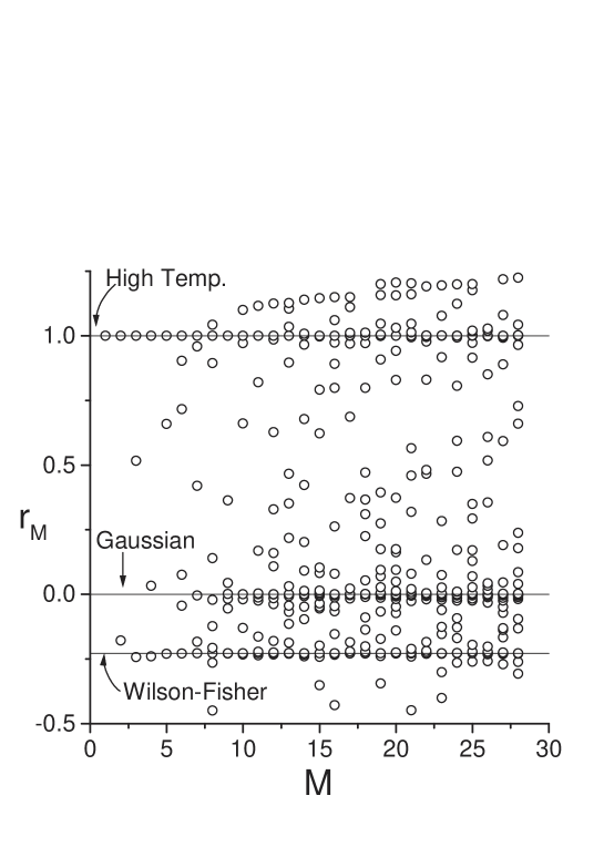
Figure 1: Distribution of the real roots $r_{M}$ (open circles) of (37) as function of the order $M$ of the Taylor series about the origin (31) [with the ADE pair $\left(w,xw^{\prime}\right)$]. A threefold accumulation occurs about the expected fixed points: trivial high temperature ($r^{\ast}=1$) and Gaussian ($r^{\ast}=0$) fixed points and about the non-trivial Wilson-Fisher fixed point ($r^{\ast}\simeq-0.2286$) [LPA, d=3].

Selection of the root

To select the right value of the root corresponding to the nontrivial Wilson-Fisher fixed point, the following procedure has been applied. We know that the root of interest is negative and real, then we select the first negative real root that appears at the smallest possible order. At the next order we choose the real root the closest to the previous choice and so on. We obtain this way with $M=28$ the following excellent estimate:

$$r^{\ast}=-0.228\,598\,202\,437\,02\,,$$ (39)

which coincides, up to the 14^th digit, with the estimate (10) obtained by the shooting method. Figure 2 shows the accuracy obtained on $r^{\ast}$ by selecting the roots this way as $M$ varies.

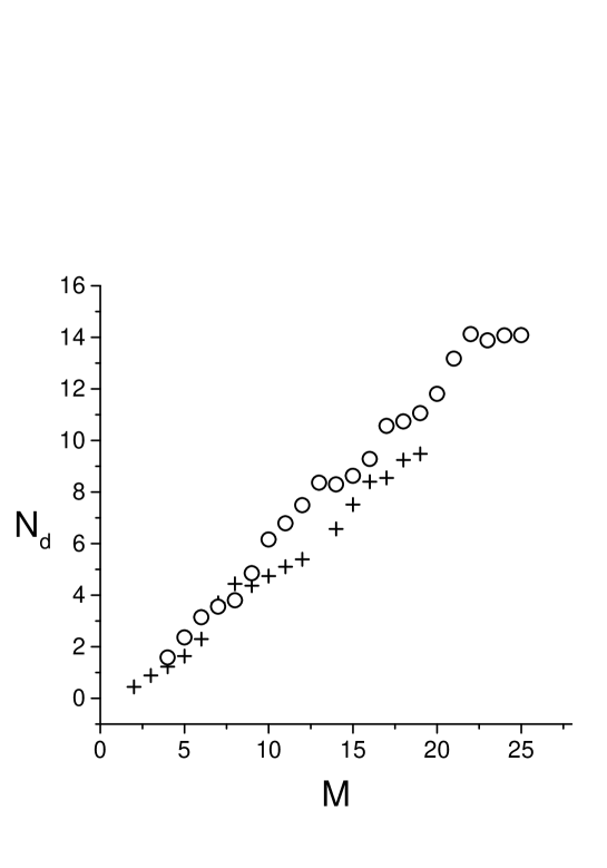
Figure 2: Approximate number of accurate digits $N_{d}=-\log\left|1-r_{M}/r^{\ast}\right|$ obtained on the selected roots $r_{M}$ as a function of $M$ and for two ADE pairs; the original $\left(w,w^{\prime}\right)$: crosses, and the variant $\left(w,xw^{\prime}\right)$: open circles [$r^{\ast}$ is given in eq. (10)]. The highest values of $M$ in each case is limited by time computing. A better efficiency is obtained with the variant.

4.1.2 Subleading high field behaviour

Equations (33, 34) used in the preceding calculations express exclusively the limit of the solution $w^{\ast}\left(x\right)$ when $x\rightarrow\infty$, and we get the unique condition (37) to estimate $r^{\ast}$. In fact there are higher correction terms to (33, 34) which vanish as $x\rightarrow\infty$ [the first of which correspond to those written in (5)]. Such subleading contributions may as well be imposed in (36). In so doing, we require the auxiliary differential equation to be satisfied not only at infinity but also in approaching this point. Consequently we obtain several auxiliary conditions similar to (37), each of them corresponding to the cancellation of the coefficient of a given power of $x.$ We have used them to determine $r^{\ast}$ again (the asymptotic constant $b$ factorizes in the first subleading conditions so obtained). The results are similar to those obtained precedently with the leading conditions (33, 34) alone. We have observed only a slight decrease in the accuracy: the higher the subleading term considered the weaker the convergence to $r^{\ast}$. This shows the coherence of the ADE method: the auxiliary condition is not an isolated point condition, it emanates from a differential equation constructed to be satisfied by the function looked for.

When the order of the subleading contribution is high enough, the constant $b$ no longer factorizes and the subleading auxiliary condition depends non trivialy on the (non-independent) integration constants ($r$ and $b$) characterizing the fixed point solution. We have tried to determine the value $b^{\ast}$ by imposing the individual vanishing of such contributions for $r=r^{\ast}$. Unfortunately, at the orders considered, the only knowledge of $r^{\ast}$ suffices to satisfy the condition (whatever the value of $b)$. It is possible that considering much higher orders would allow us to get an estimate of $b^{\ast}$ this way.

4.1.3 High field expansion and leading small field behaviour

With the determination of $b^{\ast}$ by the ADE method in view, let us perform the change of variable $x\rightarrow y^{-5}$ and the following change of function:

$$u\left(y\right)=y^{-2}\left[w\left(y^{-5}\right)-1\right]\,,$$ (40)

so that, from (5) and (29), $u^{\ast}\left(y\right)$ has the following form for small $y:$

$$u^{\ast}\left(y\right)=A^{\ast}+\frac{\,1}{5}A^{\ast 2}{y}^{2}-\frac{1}{25}A^{\ast 3}{y}^{4}+O\left(y^{5}\right)\,,$$ (41)

with

$$A^{\ast}=6b^{\ast}/5\,.$$ (42)

The fixed point differential equation (2) is then transformed into:

$$-10\,y\,{u}^{2}+5\,\left(5+2\,y^{5}\right)\,u^{\prime}-4\,\left(y^{4}-5\,y^{2}\,u^{\prime}\right)\,u+4\,y^{6}\,u^{\prime\prime}=0\,,$$ (43)

the solution of which must satisfy the following condition, see (41):

$$u^{\ast}\left(0\right) = A^{\ast}\,,$$

$$u^{\ast\prime}\left(0\right) = 0\,,$$

with $A^{\ast}$ to be determined so as, using (31, 40), to get at infinity:

$$u_{\text{asy}}^{\ast}\left(y\right)\underset{y\rightarrow\infty}{=}0\,.$$

The ADE method described in the preceding sections is used to determine the value of $A^{\ast}$. Since there are some holes in the first terms of the series (41), the first significant estimates are obtained for values of $M$ higher than in section 4.1.1. Figure (3) shows that the selected sequence of roots corresponding to $A^{\ast}$ converges to $-2.73532$ whereas, according to (9, 42), the right value expected from the shooting method is $-2.78195$.

Figure 3: In the Wilson-Polchinski case, $A^{\ast}$ does not converge (dots) to the right value $-2.78195$ (horizontal line) but to $-2.73532$.

This failure of the ADE method in determining correctly $A^{\ast}$ is presumably due to the zero radius of convergence of the Taylor series of $u^{\ast}\left(y\right)$ about $y=0$. Actually, we have estimated this radius as the limit of the ratio of two consecutive terms and observed that it goes slowly but continuously to zero as the order $M$ increases. This contrasts with the case of $w\left(x\right)$ for which the same procedure quickly tends to the following finite limit for the fixed point solution corresponding to (10, 39):

$$R_{WP}=5.721\,67\,.$$ (44)

Notice that, although the ADE method does not provide the right estimate of $A^{\ast}$ (or $b^{\ast}$), it gives a value close enough to it to be used as a guess in the shooting method.

4.2 Litim’s fixed point

4.2.1 Small field expansion and leading high field behaviour

For convenience we perform the following change, compared to section 2.2:

$$V\left(\varphi\right)=\bar{w}\left(\varphi^{2}\right)-\frac{1}{3}\,,$$ (45)

so that the fixed point equation corresponding to (19) reads (with $\bar{x}=\varphi^{2}$):

$$3\,\bar{w}-\bar{x}\,\bar{w}^{\prime}-\frac{1}{1+2\,\bar{w}^{\prime}+4\,\bar{x}\,\bar{w}^{\prime\prime}}=0\,.$$ (46)

The singularity at $\bar{x}=0$ of this second order ODE allows us to look for an analytic solution which satisfies, in terms of a single unknown parameter $\bar{k}$, the following conditions at the origin:

$$\bar{w}\left(0\right) = \bar{k}\,,$$ (47)

$$\bar{w}^{\prime}\left(0\right) = \frac{1}{6\bar{k}}-\frac{1}{2}\,,$$ (48)

with $\bar{k}$ adjusted to $\bar{k}^{\ast}$ so as to reach at infinity [from (22)]:

$$\bar{w}_{\mathrm{asy}}^{\ast}(\bar{x})=b_{L}^{\ast}\,{\bar{x}}^{3}+\frac{1}{150\,b_{L}^{\ast}\,{\bar{x}}^{2}}-\frac{1}{6300\,b_{L}^{\ast 2}\,{\bar{x}}^{4}}+O\left({\bar{x}}^{-6}\right)\,.$$ (49)

The expected value of $\bar{k}^{\ast}$ is related to $r_{L}^{\ast}$ given in (26) as:

$$\,\bar{k}^{\ast}=\frac{1}{3\left(1+\,r_{L}^{\ast}\right)}\,.$$

It is also related to $k^{\ast}$ given in (11) via (24, 45) as $\bar{k}^{\ast}=k^{\ast}+1/3$. Consequently the estimation by the shooting method is:

$$\,\bar{k}^{\ast}=0.409\,532\,734\,\allowbreak 145\,674\pm 10^{-15}\,.$$ (50)

The object of this section is thus to test whether the ADE method yields that value of $\,\bar{k}^{\ast}$ [and also that of $b_{L}^{\ast}$ given in (23)].

Contrary to the Wilson-Polchinski case, the asymptotic behaviour (49) does not reach a finite value when $\bar{x}\rightarrow\infty$. But the third derivative of $\bar{w}^{\ast}$ does. Hence, since $b_{L}^{\ast}$ is still supposed unknown, the auxiliary first order differential equation (35) may be used with $w$ and $w^{\prime}$ replaced respectively by $\bar{w}^{(4)}$ and $\bar{w}^{(5)}$ (where $\bar{w}^{(n)}$ stands for d${}^{n}\bar{w}/$d$\bar{x}^{n}$). Actually, both of these two derivatives go to zero as $\bar{x}\rightarrow\infty$ so that finally the auxiliary condition similar to (37), but with another normalisation of the $G_{i}$’s (e.g. $G_{2}=1$), reduces to:

$$G_{1}\left(\bar{k}\right)=0\,,$$ (51)

whereas the function $\bar{w}\left(\bar{x}\right)$ is expanded up to order $M$ in powers of $\bar{x}$ and inserted into (46) to get the solution at this order as function of $\bar{k}$:

$$\bar{w}_{M}\left(\bar{k};\bar{x}\right)=\bar{k}+\sum\limits_{n=1}^{M}a_{n}\left(\bar{k}\right)\bar{x}^{n}\,.$$ (52)

Similarly to the Wilson-Polchinski case, the complete set of real roots of (51) shows accumulations about the expected fixed point values. However the selection process described previously fails in picking the right value $\bar{k}^{\ast}$ (of the nontrivial fixed point) although it is present among the roots. Actually, for $M=14$ the selection gives $0.409\,627\,819\,729\,71$ whereas a better value ($0.409\,532\,733\,212\,35$) exists at the same order [compare with (50)]. The variant utilised in the preceding case which consists in replacing $\bar{w}^{(5)}$ by $\bar{x}\bar{w}^{(5)}$ does not circumvents this difficulty.

If instead of $\left(\bar{w}^{(4)},\bar{w}^{(5)}\right)$ as ADE pair, we consider the combination $h=3\,\bar{w}-\bar{x}\,\bar{w}^{\prime}$ and its derivative $h^{\prime}$ with respect to $\bar{x}$ (or the variant $\bar{x}h^{\prime}$ to save some time computing), then the new pair, according to (49), vanishes also as $\bar{x}\rightarrow\infty$ , and we observe, this time, that the selection process works again. This way, at order $M=19$ the selection gives:

$$\bar{k}^{\ast}=0.409\,532\,734\,16\,,$$

a value which coincides with (50) up to the 10^th digit. No doubt that considering higher values of $M$ would have improved the accuracy. We note that, as with Wilson-Polchinski’s function, the radius of convergence of the Taylor series of $\bar{w}\left(\bar{x}\right)$ about the origin is finite, and is about:

$$R_{L}\simeq 11.5\,.$$ (53)

Let us specify however that, contrary to the Wilson-Polchinski case, the test of the ratio $a_{i}/a_{i+1}$ of two consecutive terms of the Taylor series about the origin does not converge. We have obtained (53) by explicitly performing a partial summation of the series and studying it as a function of $\bar{x}$. Nevertheless, we have also observed that the ratio $\left|a_{i}/a_{i+3}\right|$ raised to the power $1/3$, roughly converges to (53). This remark will have some importance in section 5.4.

Since expansions I and II work in the Litim case (see [26]), we can compare the ADE method with those two methods. Figure (4) shows the respective accuracies obtained on $\bar{k}^{\ast}$ with the three methods as functions of the order $M$ of the field expansion. One sees that expansion II and the ADE method provide better results than expansion I (which likely does not converge) and that the ADE method is most efficient than expansion II (we have not studied expansion III).

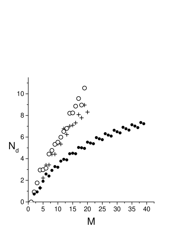
Figure 4: Approximate number of accurate digits $N_{d}=-\log\left|1-\bar{k}_{M}/\bar{k}^{\ast}\right|$ [with $\bar{k}^{\ast}$ given by (50)] as functions of $M$ for the estimations of the Litim fixed point value of $\bar{k}$ using three methods: expansion I (black dots), expansion II (crosses), and ADE (open circles). A better efficiency is obtained with the ADE method.

4.2.2 Subleading high field behaviour

As in the case of Wilson-Polchinski’s equation, the subleading terms in (49) may be used to impose the auxiliary condition not only at infinity but also in approaching this point whatever the value of $\bar{x}$. We observe the same phenomenon as in section 4.1.2: the higher the subleading term considered the weaker the convergence to $\bar{k}^{\ast}$ whereas $b_{L}^{\ast}$ cannot be determined by imposing the individual vanishing of the subleading contributions for $\bar{k}=\bar{k}^{\ast}$.

However, the fact that the asymptotic behaviour (49) is an integer power of $\bar{x}$ provides us with the oportunity of determining $b_{L}^{\ast}$ from the knowledge of $\bar{k}^{\ast}$ as a boundary limit (a point condition). Actually, since $\bar{w}^{(3)}\rightarrow 6b_{L}^{\ast}\,$ when $\bar{x}\rightarrow\infty$, we may choose $\left(\bar{w}^{(3)},\bar{w}^{(4)}\right)$ as ADE pair [or the variant $\left(\bar{w}^{(3)},\bar{x}\bar{w}^{(4)}\right)$], and for $\bar{k}$ fixed to $\bar{k}^{\ast}$ solve for $b_{L}^{\ast}$ the resulting auxiliary condition at infinity. The accuracy on $b_{L}^{\ast}$ obtained this way is not as large as in the case of $\bar{k}^{\ast}$, nevertheless, for $M=31$ we obtain the following estimation:

$$b_{L}^{\ast}\simeq 0.001\,007\,,$$ (54)

which is rather close to the shooting value (23). We indicate also that rough estimates of $b_{L}^{\ast}$ already sufficiently accurate to be used as guesses in the shooting method are obtained for small values of $M$, e.g.: $0.000\,989$ for $M=11$ or even $0.0012$ for $M=5$.

4.2.3 High field expansion and leading small field behaviour

With a view to determining $b_{L}^{\ast}$ directly by the ADE method, we invert the boundaries by changing the variable $\bar{x}\rightarrow\bar{y}^{-1}$ and by performing the following change of function:

$$\bar{u}\left(\bar{y}\right)={\bar{y}}^{3}\bar{w}\left(\frac{1}{\bar{y}}\right)\,,$$ (55)

so that, from (49), we deduce that $\bar{u}^{\ast}\left(\bar{y}\right)$ has the following form for small $\bar{y}:$

$$\bar{u}^{\ast}\left(\bar{y}\right)=b_{L}^{\ast}\,+\frac{{\bar{y}}^{5}}{150\,b_{L}^{\ast}\,}-\frac{{\bar{y}}^{7}}{6300\,b_{L}^{\ast 2}\,}+O\left({\bar{y}}^{9}\right)\,.$$ (56)

The differential equation for $\bar{u}\left(\bar{y}\right)$ is:

$$\bar{y}^{4}+18\,\bar{y}\,\left(\bar{u}^{\prime}\right)^{2}-\bar{u}^{\prime}\left[30\,\bar{u}+\bar{y}^{2}\,\left(1+4\,\bar{u}^{\prime\prime}\right)\right]=0\,.$$

The solution must satisfy the following condition at the origin $\bar{y}=0$ [see (56)]:

$$\bar{u}^{\ast}\left(0\right) = b_{L}^{\ast}\,,$$

$$\bar{u}^{\ast\prime}\left(0\right) = 0\,,$$

with $b_{L}^{\ast}$ to be determined so as, using (47, 48, 55), to get at infinity:

$$\bar{u}_{\text{asy}}^{\ast}\left(\bar{y}\right)=\bar{k}^{\ast}{\bar{y}}^{3}+\left(\frac{1}{6\bar{k}^{\ast}}-\frac{1}{2}\right){\bar{y}}^{2}+O\left(\bar{y}\right)\,.$$

As previously, we use the ADE method with a view to determining the value of $b_{L}^{\ast}\,$. For this we consider, the pair $\left(\bar{u}^{(4)},\bar{u}^{(5)}\right)$ which vanishes at infinity ($\bar{y}\rightarrow\infty$). Since there are some holes in the first terms of the series about the origin, see (56), the first significant estimates are obtained for values of $M$ higher than with the original function $\bar{w}\left(\bar{x}\right)$. Although the positive roots obtained for $b_{L}$ (we know that $b_{L}^{\ast}$ is positive) have the right order of magnitude compared to (23) the apparent convergent sequences do not provide the right value. Again, as in the Wilson-Polchinski case, we think that the failure of the ADE method is due to the (observed) zero radius of convergence of the Taylor series for $\bar{u}\left(\bar{y}\right)$ about the origin.

4.3 Eigenvalue estimates

Let us consider the eigenvalue problem with the ADE method. This time two coupled nonlinear ODEs have to be solved together (the fixed point equation and the linearisation of the flow in the vicinity of the fixed point). We can solve these two equations together as the order of the field expansion $M$ grows or consider separately the eigenvalue equation after having solved the fixed point equation with some accuracy. With the aim to be short, we present only the latter possibility which illustrates well the property of convergence of the method.

4.3.1 Wilson-Polchinski’s eigenvalues

Small field expansion and leading high field behaviour

Using a change of eigenfunction, $g\rightarrow\mathrm{v}$, similar to (29) for the fixed point function, it comes:

• in the even case:

  $$g^{\prime}\left(\phi\right)=\phi\,\mathrm{v}\left(\phi^{2}\right)\,,$$

  and eq. (13) yields the following behaviour at large $x=\phi^{2}$:

  $$\mathrm{v}_{\text{asy}}\left(x\right)=\frac{2\left(3-\lambda\right)}{5}S_{0}\,x^{-\left(2+\lambda\right)/5}\left[1+O\left(x^{-2/5}\right)\right]\,.$$

• in the odd case:

  $$g^{\prime}\left(\phi\right)=\,\mathrm{v}\left(\phi^{2}\right)\,,$$

  and eq. (13) gives:

  $$\mathrm{v}_{\text{asy}}\left(x\right)=\frac{2\left(3-\lambda\right)}{5}S_{0}\,x^{\left(1-2\lambda\right)/10}\left[1+O\left(x^{-2/5}\right)\right]\,.$$

The arbitrariness of the global normalisation of the eigenfunctions allows to choose $\mathrm{v}\left(0\right)=1$ (even) and $\mathrm{v}^{\prime}\left(0\right)=1$ (odd) corresponding respectively to some definite values of $S_{0}$. So defined, the functions $\mathrm{v}\left(x\right)$ and $\mathrm{v}^{\prime}\left(x\right)$ vanish at infinity provided that $\lambda>-2$ in the even case and $\lambda>1/2$ in the odd case. Hence one could expect that, with the simple condition at infinity: $\mathrm{v}=\mathrm{v}^{\prime}=0$ imposed in the auxiliary differential equation, the ADE procedure will, at best, allow the determination of exclusively the leading ($\lambda_{1}=1/\nu$) and first subleading ($\lambda_{2}=-\omega_{1}$) eigenvalues in the even case and of only the trivial eigenvalue $\breve{\lambda}_{1}=-\breve{\omega}_{1}$ in the odd case [see the values of these quantities in eqs. (17, 18) and tables (3, 4)]. Actually it is better than that since, as $M$ grows, we observe among the real roots of the auxiliary condition for $\lambda$ that a hierarchy of successive accumulations takes place about the right values of the leading and subsequent eigenvalues [see figure 5].

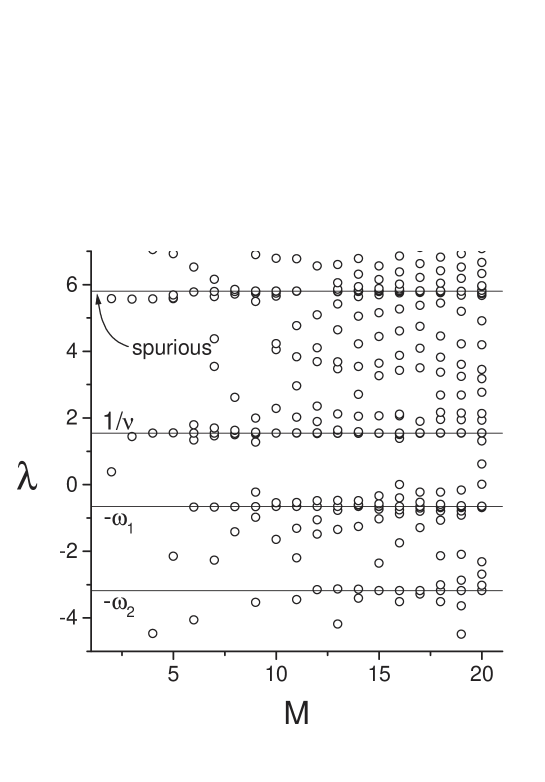
Figure 5: Accumulations of real roots (open circles) of the auxiliary condition (37) about eigenvalues as the order $M$ of the series varies in the Wilson-Polchinski even case. From top to bottom: $\lambda_{1}=1/\nu$ (second horizontal line), $\lambda_{2}=-\omega_{1}$ (third h. line) and $\lambda_{3}=-\omega_{2}$ (fourth h. line). A simple criterion of choice allows to determine their estimates at $M=20$, see the values in eqs. (57–59). An accumulation also occurs about the spurious value 5.8 (first h. line).

Within each of these accumulations of real roots, we have been able to follow without ambiguity a convergent sequence to the right estimate. At order $M=20$ with the ADE pair $\left(\mathrm{v},\mathrm{v}^{\prime}\right)$ supposed to vanish at infinity, and $r^{\ast}$ fixed to the value given in (39), we have obtained the following estimates in the even case

$$\nu = 0.649\,561\,773\,86\,,$$ (57)

$$\omega_{1} = 0.655\,745\,92\,,$$ (58)

$$\omega_{2} = 3.178\,,$$ (59)

where the number of digits has been truncated with regard to the accuracy of the estimates obtained [by comparison with (16) and table 3]. We see that the accuracy decreases as the order of the eigenvalue grows but also that we obtain an estimate of $\omega_{2}$ whereas for that value $\mathrm{v}$ does not vanish at infinity.

The same kind of observations stands in the odd case. We take the opportunity to indicate that choosing the ADE pair $\left(f,f^{\prime}\right)$ with $f=$ $\frac{\left(1-2\lambda\right)}{10}\mathrm{v}$-$x\mathrm{v}^{\prime}$ makes  $f$ vanish for $\lambda>-3/2$ and the procedure gives a better accuracy on $\breve{\omega}_{1}$ than with the pair $\left(\mathrm{v},\mathrm{v}^{\prime}\right)$. This way we obtain the following estimate [at order $M=20,$ compare with (18)]

$$\breve{\omega}_{1}=1.886\,718\,.$$

We have also noted the presence of accumulations of real roots about spurious positive values of order 5.8 in the even case and 3.77 in the odd case.

4.3.2 Litim’s eigenvalues

The determination using the ADE method of the eigenvalues from the Litim flow equation follows the same lines as previously for the Wilson-Polchinski flow equation. We limit ourselves in this section to a brief presentation of the main differences encountered.

Small field expansion and leading high field behaviour

Compared to (27), we perform a change of eigenfunction, $h\rightarrow\,\mathrm{v}_{L}$, according to the symmetry considered:

• in the even case:

  $$h\left(\varphi\right)=\,\mathrm{v}_{L}\left(\varphi^{2}\right)\,,$$

  then eq. (28) yields the following behaviour at large $\bar{x}=\varphi^{2}$:

  $$\mathrm{v}_{L\text{asy}}\left(\bar{x}\right)=S_{1}{\bar{x}}^{\,\left(3-\lambda\right)}\left[1+O\left(\bar{x}^{-5}\right)\right]\,.$$

• in the odd case:

  $$h\left(\varphi\right)=\varphi\,\mathrm{v}_{L}\left(\varphi^{2}\right)\,,$$

  and eq. (28) gives:

  $$\mathrm{v}_{L\text{asy}}\left(\bar{x}\right)=S_{1}{\bar{x}}^{\,\left(5/2-\lambda\right)}\left[1+O\left(\bar{x}^{-5}\right)\right]\,.$$

So defined, the two functions $\mathrm{v}_{L}\left(\bar{x}\right)$ and $\mathrm{v}_{L}^{\prime}\left(\bar{x}\right)$ vanish at infinity provided that $\lambda>3$ in the even case and $\lambda>5/2$ in the odd case (whereas the arbitrary global normalisation of the eigenfunctions allows to choose $\mathrm{v}_{L}\left(0\right)=1$ (even) and $\mathrm{v}_{L}^{\prime}\left(0\right)=1$ (odd) corresponding respectively to specific values of $S_{1}$).

Although it works, the original ADE pair $\left(\mathrm{v}_{L},\mathrm{v}_{L}^{\prime}\right)$ is not the most efficient choice to obtain estimates of the first nontrivial eigenvalues. A better choice appears to be the pairs $\left(f\left(\bar{x}\right),f^{\prime}\left(\bar{x}\right)\right)$ with $f\left(\bar{x}\right)=\left(3-\lambda\right)\mathrm{v}_{L}\left(\bar{x}\right)-\bar{x}\mathrm{v}_{L}^{\prime}\left(\bar{x}\right)$ in the even case and $f\left(\bar{x}\right)=$ $\left(5/2-\lambda\right)\mathrm{v}_{L}\left(\bar{x}\right)-\bar{x}\mathrm{v}_{L}^{\prime}\left(\bar{x}\right)$ in the odd case (they correspond to eigenfunctions which vanish as $\bar{x}\rightarrow\infty$ for more negative values of $\lambda$). With these choices and $\bar{k}^{\ast}=0.409\,532\,734\,145\,7$ we identify immediately the trivial eigenvalues $\lambda_{0}=3$ in the even case and $\breve{\lambda}_{1}=2.5$, $\breve{\lambda}_{2}=0.5$ in the odd case but also, for $M=20$, we obtain good estimates of the nontrivial leading and first subleading eigenvalues:

$$\begin{array}[]{llll}\nu=\allowbreak 0.649\,561\,774,&\omega_{1}=0.655\,745\,5,&\omega_{2}=3.180\,008,&\omega_{3}=5.896,\\ \breve{\omega}_{1}=1.886\,703\,7,&\breve{\omega}_{2}=4.524\,1\,,&&\end{array}$$

where the numbers of digits have been limited with respect to the estimated accuracy [compare with (16), table 3 (even) and (18), table 4 (odd)]. For each eigenvalue, the successive estimates may be followed unambiguously step by step when $M$ grows so that the right values may be easily selected following the rules defined precedently.

We notice also the presence of spurious convergences and especially in the even case to the value about 5.8 already encountered with the Wilson-Polchinski case.

5 Approximating by hypergeometric functions (HFA)

The ADE method is most certainly efficient in many cases but it is relatively heavy regarding the computing time whereas the current methods, when they work, are lighter. In addition, none of these methods provides a global solution to the ODE studied: they yield an approximate value of the integration constant but not a function as global approximation of the solution looked for.

We propose in this section an alternative method which is lighter than the ADE method and which provides a global approximation of the solution of interest. This new method is based on the definition property of the generalized hypergeometric functions. Let us first review the definition and main properties of these functions.

5.1 Generalized hypergeometric functions

For $x\in\mathbb{C}$, a series $S=\sum_{n=0}^{\infty}a_{n}x^{n}$ is hypergeometric (see for example [32]) if the ratio $a_{n+1}/a_{n}$ is a rational function of $n$, i.e.

$$\frac{a_{n+1}}{a_{n}}=\frac{P\left(n\right)}{Q\left(n\right)}\,,$$

for some polynomials $P\left(n\right)$ and $Q\left(n\right)$.

If we factorize the polynomials, we can write:

$$\frac{a_{n+1}}{a_{n}}=\alpha_{0}\frac{\left(n+\alpha_{1}\right)\left(n+\alpha_{2}\right)\cdots\left(n+\alpha_{p}\right)}{\left(n+\beta_{1}\right)\left(n+\beta_{2}\right)\cdots\left(n+\beta_{q}\right)\left(n+1\right)}\,.$$ (60)

The factor $\left(n+1\right)$ in the denominator may or may not result from the factorization. If not, we add it along with the compensating factor in the numerator. Usually, the global factor $\alpha_{0}$ is set equal to 1.

If the set $\left\{\alpha_{i}\right\}$ includes negative integers, then $S$ degenerates into a polynomial in $x.$

When it is not a polynomial, the series $S$ converges absolutely for all $x$ if $p\leq q$ and for $\left|x\right|<1/\left|\alpha_{0}\right|$ if $p=q+1$. It diverges for all $x\neq 0$ if $p>q+1.$

The analytic continuation of the hypergeometric series $S$ with a non-zero radius of convergence is called a generalized hypergeometric function and is noted:

$${}_{p}F_{q}\left(\alpha_{1},\cdots,\alpha_{p};\beta_{1},\cdots,\beta_{q};\alpha_{0}x\right)=\frac{1}{a_{0}}S\,.$$

${}_{p}F_{q}\left(x\right)$ is a solution of the following differential equation (for $\alpha_{0}=1$):

$$\left[\theta\left(\theta+\beta_{1}-1\right)\cdots\left(\theta+\beta_{q}-1\right)-x\left(\theta+\alpha_{1}\right)\cdots\left(\theta+\alpha_{p}\right)\right]\,_{p}F_{q}\left(x\right)=0\,,$$ (61)

where

$$\theta=x\frac{d}{dx}.$$

When $p>2$ or $q>1$, the differential equation (61) is of order $\max\left(p,q+1\right)>2$. It is of second order when $q=1$ and $p=0$, $1$ or $2$. It is of first order when $q=0$ and $p=1$

${}_{2}F_{1}$ is currently named the hypergeometric function. A number of generalized hypergeometric functions have also special names: ${}_{0}F_{1}$ is called confluent hypergeometric limit function and ${}_{1}F_{1}$ confluent hypergeometric function.

In the cases $p\leq q$ for fixed $\left\{\alpha_{i}\right\}$ and $\left\{\beta_{i}\right\}$, ${}_{p}F_{q}\left(x\right)$ is an entire function of $x$ and has only one (essential) singular point at $x=\infty$.

For $p=q+1$ and fixed $\left\{\alpha_{i}\right\}$ and $\left\{\beta_{i}\right\}$ in non-polynomial cases, ${}_{p}F_{q}\left(x\right)$ does not have pole nor essential singularity. It is a single-valued function on the $x$-plane cut along the interval $\left[1,\infty\right]$, i.e. it has two branch points at $x=1$ and at $x=\infty$.

Considered as a function of $\left\{\beta_{i};i=1,\cdots,q\right\}$, ${}_{p}F_{q}\left(x\right)$ has an infinite set of singular points:

1. $\beta_{i}=-m$, $m\in\mathbb{N}$ which are simple poles

2. $\beta_{i}=\infty$ which is an essential singular point (the point of accumulation of the poles).

As a function of $\left\{\alpha_{i};i=1,\cdots,p\right\}$, ${}_{p}F_{q}\left(x\right)$ has one essential singularity at each $\alpha_{i}=\infty$.

The elementary functions and several other important functions in mathematics and physics are expressible in terms of hypergeometric functions (for more detail see [32]).

The wide spread of this family of functions suggests trying to represent the solution of the ODEs presently of interest in this article, under the form of a generalized hypergeometric function.

5.2  The HFA method

For the sake of the introduction of the new method, let us first consider the Wilson-Polchinski fixed point equation (30) and the truncated expansion (32) in which the coefficients $a_{n}\left(r\right)$ $(n=1,\cdots,M)$ are already determined as function of $r$ via a generic solution of (30) truncated at order $M$ (in powers of $x)$. The question is again to construct an auxiliary condition to be imposed with a view to determining the fixed point value $r^{\ast}$. To this end, by analogy with the generalized hypergeometric property definition recalled in section 5.1, we construct the ratio of two polynomials in $n$:

$$\frac{P_{m_{1}}\left(n\right)}{Q_{m_{2}}\left(n\right)}=\frac{\sum_{i=1}^{m_{1}}c_{i}\,n^{i-1}}{\sum_{i=1}^{m_{2}}d_{i}\,n^{i-1}}\,,$$ (62)

so that $P_{m_{1}}\left(n\right)/Q_{m_{2}}\left(n\right)$  match the $M-2$ ratios $a_{n+1}\left(r\right)/a_{n}\left(r\right)$  for $n=1,\cdots,M-2$. Hence, accounting for the arbitrariness of the global normalisation of (62), the complete determination of the two sets of coefficients $\left\{c_{i};i=1,\cdots,m_{1}\right\}$ and $\left\{d_{i};i=1,\cdots,m_{2}\right\}$ as functions of $r$ implies $m_{1}+m_{2}=M-1$. Finally, the auxiliary condition on $r$ is obtained by requiring that the last (still unused) ratio $a_{M}\left(r\right)/a_{M-1}\left(r\right)$ satisfies again the $n$-dependency satisfied by its predecessors, namely that:

$$\frac{\sum_{i=1}^{m_{1}}c_{i}\left(r\right)\left(M-1\right)^{i-1}}{\sum_{i=1}^{m_{2}}d_{i}\left(r\right)\left(M-1\right)^{i-1}}=\frac{a_{M}\left(r\right)}{a_{M-1}\left(r\right)}\,.$$ (63)

The auxiliary condition so obtained is a polynomial in $r$, the roots of which are candidates to give an estimate at order $M$ of $r^{\ast}$ (noted below $r_{M}^{\ast}$). Notice that, to obtain faster this auxiliary condition, one may avoid the calculation of the coefficients $c_{i}\left(r\right)$ and $d_{i}\left(r\right)$ by following the same considerations as those leading to (38) with the ADE method.

At this point, the method potentially reaches the same goal as the ADE and other preceding methods. However, according to section 5.1, in determining the ratio of polynomials (62) we have also explicitly constructed the function

$$F_{M}\left(x\right)=r_{M}^{\ast}\cdot\,_{m_{1}+1}F_{m_{2}}\left(\alpha_{1},\cdots,\alpha_{m_{1}},1;\beta_{1},\cdots,\beta_{m_{2}};\alpha_{0}x\right)\,,$$ (64)

in which $r_{M}^{\ast}$ is the selected estimate of $r^{\ast}$, the sets $\left\{-\alpha_{i}\right\}$ and $\left\{-\beta_{i}\right\}$ are the roots of the two polynomials $P_{m_{1}}\left(n\right)$ and $Q_{m_{2}}\left(n\right)$ when $r=r_{M}^{\ast}$ whereas:

$$\alpha_{0}=\frac{c_{m_{1}}\left(r_{M}^{\ast}\right)}{d_{m_{2}}\left(r_{M}^{\ast}\right)}\,.$$ (65)

Now, by construction, $F_{M}\left(x\right)$, has the same truncated series in $x$ as the solution of (30) we are looking for. This function is thus a candidate for an approximate representation of this solution.

It is worth noticing that, contrary to the ADE method, the HFA method does not make an explicit use of the conditions at infinity (large $x$) to determine $r^{\ast}$. Only a local information, in the neighbourhood of the origin $x=0$, is explicitly employed.

Let us apply the method to the two equations of interest in this paper.

5.3 Wilson-Polchinski’s equation

5.3.1 Fixed point

We know that the absolute value of the ratio $a_{n}\left(r^{\ast}\right)/a_{n+1}\left(r^{\ast}\right)$ has a definite value $R_{WP}$ [given by eq. (44)] as $n\rightarrow\infty$. Consequently, we must consider the ratio (62) with $m_{1}=m_{2}$ (this implies also that $M$ be odd). In this circumstance, according to section 5.1, the relevant hypergeometric functions have a branch cut on the positive real axis (as functions of $\alpha_{0}x$). Consequently the analytic continuation to large positive values of $x$ is only possible if $\alpha_{0}<0$. We note also that, according to (44), $\left|\alpha_{0}\right|$ should converge to $1/R_{WP}=0.174774$. Finally by considering the large $x$ behaviour directly on (61), it is easy to convince oneself that the leading power is given by one of the parameters $\left\{-\alpha_{i}\right\}$, consequently we expect to observe a stable convergent value among the $\alpha_{i}$’s toward the opposite of the leading power at large $x$ of the solution looked for. For this reason, instead of the function $w\left(x\right)$ of section 4.1.1 the limit of which is 1 as $x\rightarrow\infty$ [see (33)], we have considered the translated function $w_{t}\left(x\right)=w\left(x\right)-1$ which, according to eqs (5) and (29, 42), tends to $A^{\ast}x^{-2/5}$. In this case we thus expect to observe a stable value among the $\alpha_{i}$’s about $0.4$ with the eventual possibility of estimating $A^{\ast}$.

When looking at the roots of the auxiliary condition (63) as $M$ varies, we obtain the same kind of accumulations about the expected fixed point value $r^{\ast}$ as shown in figure 1 (with much less points however). We can also easily select the right nontrivial solution using the procedure described just above (39). We get precisely this excellent estimate with $M=25$ and a reduced computing time compare to the ADE method. Figure (6) shows the accuracies obtained on $r^{\ast}$ (crosses) compared to the ADE method (open circles).

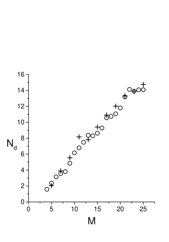
Figure 6: Respective approximate number of digits (defined in the caption of figure 2) obtained for r${}_{M}^{\ast}$ with the HFA method (crosses) and the ADE method (open circles) for the Wilson-Polchinski fixed point equation. Whereas at a given order $M$ the accuracy is similar, a smaller time computing is necessary with the HFA method.

Furthermore, the sets of parameters of the successive hypergeometric functions involve two stable quantities the values of which at $M=25$ are:

$$\alpha_{0} = -0.174\,775\,,$$ (66)

$$\alpha_{1} = 0.396\,2\,.$$ (67)

Those two results are quantitatively and qualitatively very close to the expected values (respectively $-0.174774$ and $0.4$ as given just above).

This clearly shows that the hypergeometric function determined this way provides us with a really correct (but approximate) global representation of the fixed point function. This contrasts strongly with the numerical integration of the ODE which, due to the presence of the moving singularity, never provides us with such an approximate global representation of the solution looked for.

From (67) we have obtained a rough estimate of $A^{\ast}$ ($=6b^{\ast}/5$) by a direct consideration of the value of the corresponding function $F_{M}\left(x\right)$ defined in (64) for some relatively large value of $x$ and we obtain $A^{\ast}\simeq-2.6$ what is a sufficiently accurate estimate to serve as a guess in the shooting method.

We have also tried to determine, using the HFA method, the value $A^{\ast}$ directly from the “reverse side” corresponding to (43). We have not improved the previous biased estimate obtained by ADE (about $A^{\ast}=-2.735$). We do not understand the significance of this coincidence. We recall, however, that the radius of convergence of the Taylor series of $u^{\ast}\left(y\right)$ about $y=0$ probably vanishes. This biased result shows again that the property of convergence of the Taylor series is crucial for the accuracy of the two methods.

5.3.2 Eigenvalues

We have also applied the HFA method to the determination of the eigenvalues. With $M=17$, we have easily and without ambiguity obtained the following excellent estimates [compare with (16, 18) and tables 3 and 4]:

$$\begin{array}[]{lll}\nu=\allowbreak\allowbreak 0.649\,561\,774\,,&\omega_{1}=0.655\,745\,939\,3\,,&\omega_{2}=3.180\,006\,53\,,\\ \omega_{3}=5.912\,229\,4\,,&\omega_{4}=8.796\,045\,,&\omega_{5}=11.800\,4\,,\\ \breve{\omega}_{1}=1.886\,703\,839\,,&\breve{\omega}_{2}=4.524\,390\,3\,,&\breve{\omega}_{3}=7.337\,635\,.\end{array}$$

These results show a greater efficiency than with the ADE method especially in the determination of the subleading eigenvalues.

It is worth indicating also that, surprisingly enough, we observe again (i.e. as with the ADE method) the presence of convergences to the same spurious eigenvalues: 5.8 and 3.8 in the even and odd cases respectively.

5.4 Litim’s equation

5.4.1 Fixed point

Applying the HFA method with the ratio of two successive coefficients $a_{n}\left(\bar{k}\right)$ provides again an accumulation of roots about the right value of $\bar{k}^{\ast}$ given in (50). However, this time, we have encountered some difficulties in defining a process of selection of the right root. We obtain the following estimate for $M=21$:

$$\bar{k}^{\ast}\simeq 0.409\,531\,,$$

which is not bad [compare with (50)] but not as satisfactory as in the preceding Wilson-Polchinski’s case.

With regard to the transformation (20) and the preceding success of the HFA method, it is not amazing that the representation of the solution in the Litim case be more complicated than in the Wilson-Polchinski case.

We have already mentioned that, instead of the ratio of two successive terms of the series $a_{n}\left(\bar{k}\right)$, it is a shifted ratio that roughly converges to the finite radius of convergence (53). As a matter of fact, if we use the ratios

$$\frac{a_{n+3}\left(\bar{k}\right)}{a_{n}\left(\bar{k}\right)}\,,$$

instead of the ratio $a_{n+1}/a_{n}$ without changing the procedure described in section 5.2, then we get a better estimate for $M=21$ [compare with (50)]:

$$\bar{k}^{\ast}\simeq 0.409\,532\,737\,,$$

although the convergence properties are not substantially modified.

Because the case is apparently more complicated than precedently, we do not pursued further the discussion of the global representation of the fixed point solution by generalized hypergeometric functions.

5.4.2 Eigenvalues

For the eigenvalue problem, a similar difficulty occurs where the right values do not appear as clear convergent series of roots. At order $M=17$, we get the following estimates:

$$\begin{array}[]{llll}\nu=0.649\,55\,,&\omega_{1}=0.657\,6\,,&\omega_{2}=3.20\,,&\omega_{3}=5.8\,,\\ \breve{\omega}_{1}=1.89\,,&\breve{\omega}_{2}=4.5\,.&&\end{array}$$

As in the case of the fixed point determination, if instead of applying the method with the ratio of two successive terms of the series $a_{n}\left(\bar{k}\right)$ we consider the ratios

$$\frac{a_{n+3}\left(\bar{k}\right)}{a_{n}\left(\bar{k}\right)}\,,$$

then we get better estimates for $M=19$:

$$\begin{array}[]{llll}\nu=0.649\,561\,774\,,&\omega_{1}=0.655\,75\,,&\omega_{2}=3.180\,7\,,&\omega_{3}=5.905\,,\\ \breve{\omega}_{1}=1.886\,71\,,&\breve{\omega}_{2}=4.524\,.&&\end{array}$$

where the numbers of digits have been limited having regard to the estimated accuracies [compare with (16), table 3 (even) and (18), table 4 (odd)].

6 Summary and conclusions

We have presented the details of a highly accurate determination of the fixed point and the eigenvalues for two equivalent ERGEs in the local potential approximation. First, we have made use of a standard numerical (shooting) method to integrate the ODEs concerned. Beyond the test of the equivalence between the two equations, already published in [21], the resulting numerics have been used to concretely test the efficiency of two new approximate analytic methods for solving two point boundary value problems of ODEs based on the expansion about the origin of the solution looked for (field expansion).

We have considered explicitly those two methods applied to the study of the two equivalent ODEs. We have shown that they yield estimates as accurate as those obtained with the shooting method provided that the Taylor series about the origin of the function looked for has a non-zero radius of convergence.

This is an important new result since, up to now, no such approximate analytical method was known to work in the simplest case of the Wilson-Polchinski equation. In the case of the Litim equation the two methods converge better than the currently used expansions (usually referred to as I and II in the literature, see e.g. [[14]]). Our results support concretely the conclusions of [19] which indicated that the high field contributions were important in the Wilson-Polchinski case whereas they were less important in the Litim case.

The first of the two methods relies upon the construction of an auxiliary differential equation (ADE) satisfied by the Taylor series at the origin and to which is imposed the condition of the second boundary (at infinity) [15].

The second method (HFA) is new. It consists in defining a global representation of the solution of the ODE via a generalized hypergeometric function. The HFA method provides the advantage of yielding a global (approximate) representation of the solution via an explicit hypergeometric function.

In both cases it is possible to obtain easily (with few terms in the field expansion) rough estimates of the solution which may be used as guesses in a subsequent shooting method.

The procedures may be applied to several coupled ODEs as shown in [15] for the ADE method. Hence, we hope that the present work will make easier and more efficient future explicit (and ambitious) considerations of the derivative expansion of exact renormalisation group equations.

7 Acknowledgements

We thank D. Litim for comments on an earlier version of this article.

References

- [1] M. Gell-Mann and F. E. Low, Phys. Rev. 95 (1954) 1300. K. G. Wilson, Phys. Rev. 140 (1965) B445; ibid. D 2 (1970) 1438.
- [2] K. G. Wilson, Rev. Mod. Phys. 47 (1975) 773.
- [3] J. Zinn-Justin, Euclidean Field Theory and Critical Phenomena, Fourth edition (Clarendon Press, Oxford, 2002). A. Pelissetto and E. Vicari, Phys. Rep. 368 (2002) 549.
- [4] C. Wetterich, Phys. Lett. B 301 (1993) 90. M. Bonini, M. D’Attanasio and G. Marchesini, Nucl. Phys. B 409 (1993) 441. T. R. Morris, Int. J. Mod. Phys. A 9 (1994) 2411. U. Ellwanger, Z. Phys. C 62 (1994) 503.
- [5] K.G. Wilson, Irvine Conference, 1970, unpublished. See the equation in K. G. Wilson and J. B. Kogut, Phys. Rep. 12 (1974) 75.
- [6] F. J. Wegner and A. Houghton, Phys. Rev. A 8 (1973) 401.
- [7] J. Polchinski, Nucl. Phys. B 231 (1984) 269.
- [8] K. I. Aoki, Int. J. Mod. Phys. B 14 (2000) 1249. C. Bagnuls and C. Bervillier, Phys. Rep. 348 (2001) 91. J. Berges, N. Tetradis and C. Wetterich, Phys. Rep. 363 (2002) 223. J. Polonyi, Cent. Eur. J. Phys. 1 (2003) 1. For a recent overview of advanced functional RG methods, see J. M. Pawlowski, hep-th/0512261. For a pedagogical introduction see B. Delamotte, cond-mat/0702365.
- [9] J. F. Nicoll and T. S. Chang, Phys. Lett. A 62 (1977) 287.
- [10] G. R. Golner, Phys. Rev. B 33 (1986) 7863.
- [11] A. Margaritis, G. Ódor and A. Patkós, Z. Phys. C 39 (1988) 109. Actually the procedure followed there had already been implemented in another context by F. M. Fernandez and E. A. Castro, J. Phys. A 14 (1981) L485 and by J. R. Silva and S. Canuto, Phys. Lett. A 88 (1982) 282; ibid. A 101 (1984) 326; ibid. Phys. A 106 (1984) 1.
- [12] N. Tetradis and C. Wetterich, Nucl. Phys. B 422 (1994) 541.
- [13] M. Alford, Phys. Lett. B 336 (1994) 237.
- [14] K. I. Aoki, K. Morikawa, W. Souma, J. I. Sumi and H. Terao, Prog. Theor. Phys. 95 (1996) 409; ibid. 99 (1998) 451.
- [15] B. Boisseau, P. Forgacs and H. Giacomini, J. Phys. A 40 (2007) F215.
- [16] P. Amore and F. M. Fernandez, arXiv:0705.3862 (2007).
- [17] D. F. Litim, Phys. Rev. D 64, 105007 (2001); Phys. Lett. B 486 (2000) 92.
- [18] D. F. Litim, Int. J. Mod. Phys. A 16 (2001) 2081.
- [19] D. F. Litim, J. High Energy Phys. 07 (2005) 005.
- [20] T. R. Morris, J. High Energy Phys. 07 (2005) 027.
- [21] C. Bervillier, A. Jüttner and D. F. Litim, Nucl. Phys. B 783 (2007) 213.
- [22] G. Felder, Comm. Math. Phys. 111 (1987) 101.
- [23] K. G. Wilson and M. E. Fisher, Phys. Rev. Lett. 28 (1972) 240.
- [24] W. H. Press, S. A. Teukolsky, W. T. Vetterling and B. P. Flannery, The Art of Scientific Computing (Cambridge University Press, 1992).
- [25] R. D. Ball, P. E. Haagensen, J. I. Latorre and E. Moreno, Phys. Lett. B 347 (1995) 80. J. Comellas and A. Travesset, Nucl. Phys. B 498 (1997) 539. C. Bervillier, Phys. Lett. A 332 (2004) 93.
- [26] D. F. Litim, Nucl. Phys. B 631 (2002) 128.
- [27] D. F. Litim and L. Vergara, Phys. Lett. B 581 (2004) 263.
- [28] L. Canet, B. Delamotte, D. Mouhanna and J. Vidal, Phys. Rev. B 68 (2003) 064421; ibid. D 67 (2003) 065004.
- [29] J. P. Blaizot, R. Mendez-Galain and N. Wschebor, Phys. Lett. B 632 (2006) 571; see also hep-th/0605252. D. Guerra, R. Mendez-Galain and N. Wschebor, arXiv:0704.0258.
- [30] B. Delamotte, D. Mouhanna and M. Tissier, J. Phys.: Condens. Matter 16 (2004) S883; Phys. Rev. B 69 (2004) 134413.
- [31] T. R. Morris, Phys. Lett. B 334 (1994) 355.
- [32] G. E. Andrews, R. Askey and R. Roy, Special Functions (Cambridge University Press, 1999). G. Gasper and M. Rahman, Basic Hypergeometric Series (Cambridge University Press, 2004).