Hiking the hypercube: producers and consumers

Abstract

We study the dynamics of co-evolution of producers and customers described by bit-strings representing individual traits. Individual ”size-like” properties are controlled by binary encounters which outcome depends upon a recognition process. Depending upon the parameter set-up, mutual selection of producers and customers results in different types of attractors, either an exclusive niches regime or a competition regime.

PACS: 89.65.-s Social and economic systems

1 Introduction: hikers of the hypercube

The study of dynamical systems most often concerns systems with few degrees of freedom, or spatial systems. Physicists are less concerned with other high dimensional systems. But many models in biology and the social sciences are based on bit strings of often large dimensions.

If we take the case of biology and especially genomics, the genome or the succession of monomers in biopolymers, is often represented by a bit string. This is e.g. the case for models of the origin of life [1], immunology [2], and of co-evolution [3].

These models are generally based on the following functional scheme:

$$Genome\Longrightarrow recognition\Longrightarrow action\Longrightarrow results\Longrightarrow population\quad change.$$

The ”genome” described by a bit string undergoes selective encounters with other genomes and some action with more or less successful results influences a death and/or ”birth” process.

These models also inspired social sciences: Cultural and opinion dynamics have been described by [4, 5]. The minority game [6] applies to finance. Finally the genetic algorithm approach [7] has a wide range of applications ranging from co-evolution to optimisation.

All these algorithms have in common the bit-string description and most often a recognition process, but they differ by the consequences of significant encounters, as stressed by the well known title in psychology: ”What do you do after your say Hello?”[8] .

The present model is built along the above lines. Let us consider a set of consumers possibly interested in different products which characteristics are described by bit strings. In the case of a car these characteristics could be comfort, speed, size, gas consumption etc. We here simplify by considering binary, independent characteristics.

The preferences of consumers $i$ depend upon the overlap of their own ideal string, their need string $S_{i}$, with the product set of characteristics $S_{j}$:

$$\begin{array}[]{lll}q_{ij}=\sum_{l=1}^{k}S^{l}_{i}.EQ.S^{l}_{j}\end{array}$$ (1)

Where the symbol $EQ$ stands for the logical equivalence relation, which gives 1 if the two bits are equal and 0 otherwise. The recognition condition is that the overlap is larger than a fixed threshold. Encounters and generated profits (or losses) influence an integrated continuous variable which control the survival of the agents. Our model, to be completely defined in the next section, then defines a co-evolution dynamics of consumers and producers.

We are interested in the dynamics of population of agents on the hypercube and in the stable patterns that may arise. We want to know how these patterns depend upon the parameters of the model: what are the different regimes, where are their transitions.

The model is based on a consumers/producers co-evolution (as in [9]) but it can also be applied to other domains. In political science for instance, one could model the co-evolution of political parties platforms and voters choices as described by bit strings; each bit is now the position of the party (or the voter) on some specific issue, Europe, retirement policy, environment etc.

Other applications can be very concrete. A major car constructor can in principle provide a lot of options: their combination would correspond to more than ten thousands different cars. But not all combinations would sell well; furthermore each change on the production chain has a cost. The issue for the producers is which combination of options should I propose to the public in view of its distribution of preferences. The same issue is faced by the local dealer: which stock of combinations should I keep available to the local public?

2 The Model

In the model there are $N_{p}$ producer agents and $N_{c}$ consumer agents. Each consumer prefers a product which characteristics are coded by a ”need” string of $k$ bits. Each producer manufactures a single product which characteristics are also coded by a product string of $k$ bits. The bit string of a consumer represents what the consumer agent needs and the bit string of a producer is a code for the product that he is able to supply.

In addition to the two bit strings that code for needs and products, the ”wealth” of each agent is defined by a scalar variable $S$ or $C$, depending upon the agent type (consumer or producer, respectively). The variable $S_{i}$ represents the degree of satisfaction of the consumer $i$ and $C_{j}$ represents the capital accumulated by producer $j$.

In economy this role is played by money, but in other contexts it could be power or status.

The dynamics of the model is described by:

A recognition and transaction process.

At each time step, all consumers look for the producer which product is closest to their need (the product string with the largest overlap $q_{ij}$; in the case of equality among several producers a random choice is made among them). If the relative overlap $\frac{q_{ij}}{k}$ between the producer and the consumer strings is larger than a threshold $\theta$, a transaction occurs and the consumer satisfaction is changed according to:

$$\begin{array}[]{lll}S_{i}(t+1)=S_{i}(t)-a_{c}+\frac{q_{ij}}{k}&&\end{array}$$ (2)

Satisfaction is increased according the relative overlap of the need and product strings. It is decreased by a constant cost per transaction $a_{c}$.

The equivalent updating of the producers capital is:

$$\begin{array}[]{lll}C_{j}(t+1)=C_{j}(t)-a_{p}+\sum_{i(j)}\frac{q_{ij}}{k}&&\end{array}$$ (3)

Capital is increased by the set of transactions in which producer $j$ was involved during the time interval, according the relative overlaps of the need and product strings. The index $i(j)$ runs over all the consumers $i$ that were supplied by producer $j$. Capital is decreased by a constant production cost $a_{p}$.

A death and renewal process.

There is no upper limit to consumer satisfaction or to producer capital. But due to the costs terms, they may decrease to zero.

A producer which capital would become negative is destroyed and not renewed.

On the opposite, a consumer which satisfaction would become negative disappears and is replaced by a new consumer, with a constant initial satisfaction $S_{0}$ and a randomly generated need string.

3 Checking the parameter space

In principle there are eight independent parameters:

• The string length $k$ and the threshold $\theta$ for interaction.

• The consumption constants $a_{p}$ and $a_{c}$.

• The initial numbers of producers ($N_{p}$) and consumers ($N_{c}$).

• The initial endowments of producers ($C_{p}$) and consumers ($S_{c}$).

In practice, because of the irreversibily of the producers death process, $C_{p}$ and $N_{p}$ influence mostly the early stages of the dynamics.

In terms of dynamical regimes and transitions, we might expect that the most important parameters are $a_{c}$ and $\theta$ ( since we keep $k$ constant).

In equation 1, the positive term $\frac{\theta}{k}$ is between 0 and 1. Then, for large values of $a_{c}$, $a_{c}$ larger than 1, the change in consumer satisfaction is negative: the dynamics is characterised by a renewal process of consumers. Consumers are created with $S=S_{c}$, and their satisfaction can only linearly decrease to zero when they die. On average their satisfaction is $S=S_{c}/2$. $a_{c}=1$ is then the critical value of the satisfaction parameter separating the regime where some consumers may increase their satisfaction with time and survive, from a renewal regime when all consumers are condemned to a rapid death.

The threshold for interaction $\theta$ fixes a basin of satisfaction in the neighborhood of the producer, which size is given by the number of sites $n_{s}(\theta)$ which Hamming distance to its product string is less or equal to $k-\theta$. Any consumer which string is in the basin of satisfaction of a producer may interact with her. For $k=10$, $\theta=1$ gives a neighbourhood of size 1, size 11 for $\theta=0.9$, size 56 for $\theta=0.8$ etc. Comparing $n_{s}(\theta)\times N_{p}$ to $2^{k}=1024$, the number of sites on the hypercube, gives an approximation of the condition in threshold separating the competition regime at low $\theta$ values, from the ”niche” regime. In the competition regime, customers may choose between different producers in their neighborhood; producers then competes for customers. In the niche regime, they are so far apart that they don’t compete.

In the competition regime, according to $a_{p}$ values, we might predict that competition will reduce a too large initial number of producers by bankruptcy, until they get closer to the critical number where the niche regime is established. But according to initial conditions, essentially $C_{p}$ and $N_{p}$, the selection of surviving producers may end up in a variety of attractors as shown by simulations. Anyway, a maximum number of surviving producers in the competition regime can be estimated from equation 3. At equilibrium:

$$\begin{array}[]{lll}a_{p}=\frac{N_{c}}{N_{p}}\frac{<q_{ij}>}{k}\\ N_{p}=\frac{N_{c}}{a_{p}}\frac{<q_{ij}>}{k}&&\end{array}$$ (4)

These equations are based on an approximation of uniform distribution of product strings on the hypercube. On average each producer is surrounded by $\frac{N_{c}}{N_{p}}$ customers which contribute to its capital balance. We will further observed that this upper bound is seldom reached.

4 Simulation results

Most simulations were made for a fixed set of parameters: String length $k=10$, producers cost constant $a_{p}=4.5$, number of consumers ($N_{c}$=1000) and initial endowments of producers ($C_{p}=200$) and consumers ($S_{c}=5$). Simulation times were usually 2000, but we checked that the stationary regime was reached by increasing simulation times up to 10000.

We studied the influence of consumers constant $a_{c}$, threshold $\theta$ and $N_{p}$ the initial number of producers.

4.1 Time evolution

Let us first monitor the time evolution of producers capital $C_{i}$, of the average consumer satisfaction $S$, of the number of consumers death per time unit and of the surviving number of producers.

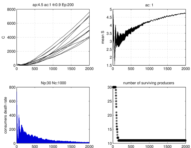
Figure 1: Time evolution of producers capital $C_{i}$, of the average consumer satisfaction $S$, of the number of consumer death per time unit and the number of surviving producers. $N_{p}$ initial was 30, $N_{c}=1000$, $a_{c}=1$, $C_{p}=200$, $\theta=.9$.

On figure 1, where $N_{p}$ initial was 30, $N_{c}=1000$, $a_{p}=1$, $\theta=.9$, we see on the lower right curve that producers are first selected: there number is decreased from 30 to 11, and then business becomes profitable ($C$ evolution, on the upper left curves). The early producer selection gives figures much lower that the upper bound computed by equation 3 (which should be around 200), but surviving producers make profit.

Consumers average satisfaction is always lower than 5: since $a_{c}=1$ no consumer ever increase satisfaction alive, but the random generation of reborn consumers allow some of them, ”the condensed” consumers, to reach the cell of one producer where they may survive for ever. Average $S$ reflects the division between a fraction $f$ of condensed consumers with $S=5$ and of starving consumers with average $S=2.5$. $f$ then obeys:

$$f\times 5+(1-f)\times 2.5=<S>$$ (5)

$$f=\frac{<S>-2.5}{2.5}$$ (6)

The increase of $<S>$ towards 5 with time then reflects the increase of the fraction of ”condensed” consumers towards 1. This effect is confirmed by decrease of the death rate on the lower left plot.

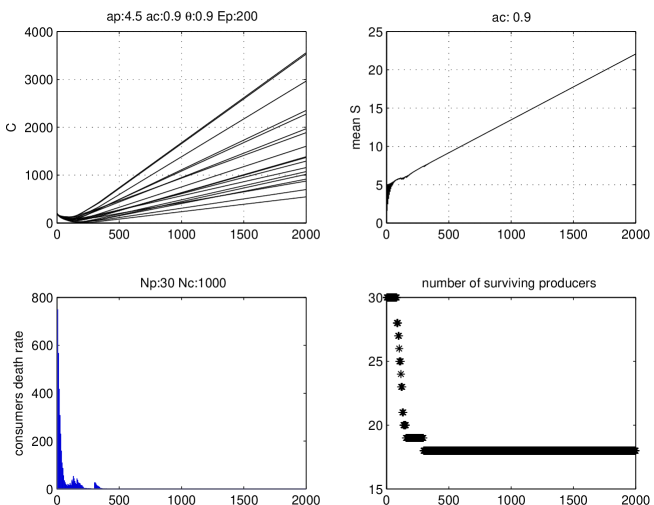
Figure 2: Time evolution of producers capital $C_{i}$, of the average consumer satisfaction $S$, of the number of consumer death per time unit and of the number of surviving producers strings. $N_{p}$ initial was 30,$N_{c}=1000$, $\theta=.9$, $C_{p}=200$, as on the previous figure but the product cost is now $a_{p}=0.9$ instead of 1.

With $a_{p}=0.9$, smaller than one, those condensed consumers in the neighborhood of the producers can even increase satisfaction during their infinite lifetime as observed on the right upper corner. Because of the lower stress on consumers, they early find spots where they are able to survive, and they stabilize in the neighborhood of producers much earlier in time. The diversity of producers is higher: 17 survive.

4.2 Attractors

Let us now do a systematic study of the attractors of the dynamics. We checked the asymptotic state of the system through a similar set of variables: producers capital $C_{i}$, average consumer satisfaction $<S>$, number of surviving producers.

We also tried to characterise the degree of order or of diversity of the attractor configuration and used the overlap of buyers need strings as the order function. This is the same notion as used in spin glass theory. We then checked the fraction $\frac{h(10)}{h(5)}$ of the histogram of overlaps among buyers need strings. This gives us an indication about how many consumers are condensed and what is their repartition (even or uneven) in the neighborhood of producers.

In the next four figures, the horizontal variable is $N_{p}$ the initial number of producers. The four set of figures correspond to two values of $\theta$, 09 and 0.8, and $a_{p}$, 0.9 and 1. These results were averaged over 100 different random samplings of initial configurations.

There is not much to add about the influence $a_{p}$ from these figures.

But the influence of $\theta$ on the transition between a competition regime ($\theta=.8$) and a niche regime ($\theta=.9$) is now made clear.

In the niche regime, $\theta=.9$, few producers survive, even for large initial number of producers (figure 3). Their number saturates around 20 for higher values of the initial producer number. Producers make a lot of profit (large $C$ values) (figure 4).

Consumers satisfaction depends upon $a_{c}$ (figure 5).

Significant values of $h(1)$ are observed when $a_{c}$ and $\theta$ are both large.

Figure 3: Number of surviving producers. These are taken at time=2000. $N_{p}$ is varied along the x axis (logarithmic scale). Each of the four plots correspond to a given pair of $a_{p}$ and $\theta$ values, upper plots to a threshold $\theta=0.8$ lower plots to a threshold $\theta=0.9$, left plots to consumption $a_{c}=1$ and right plots to consumption $a_{c}=0.9$.

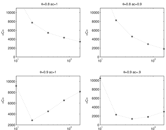
Figure 4: Averaged producer capital $C_{i}$ at time=2000. $N_{p}$ is varied along the x axis (logarithmic scale). Each of the four plots correspond to a given pair of $a_{p}$ and $\theta$ values.

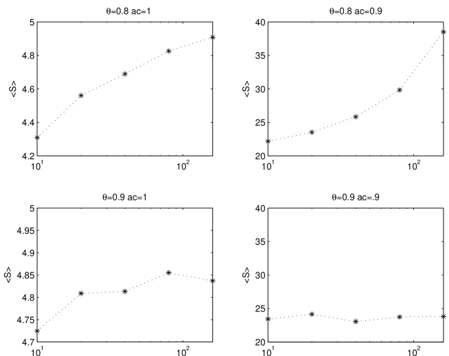
Figure 5: Average consumer satisfaction $S$ at time=2000. $N_{p}$ is varied along the x axis (logarithmic scale). Each of the four plots correspond to a given pair of $a_{c}$ and $\theta$ values, upper plots to a threshold $\theta=0.8$ lower plots to a threshold $\theta=0.9$, left plots to consumption $a_{c}=1$ and right plots to consumption $a_{c}=0.9$.

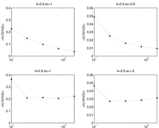
Figure 6: Relative size of the condensed fraction ( $\frac{h(10)}{h(5)}$) of consumers at time=2000. $N_{p}$ is varied along the x axis (logarithmic scale).

On figure 6, the large value of the 10 overlap bin observed when $a_{c}=1$ and $\theta=.9$ is an indication that many customers have the same need string. This concentration of need strings, co-occuring with small number of surviving producers, is obviously due to their ”condensation” on producers ”product” strings. Furthermore, the large value of 0.2 observed for $a_{c}=1$ and $\theta=0.9$ tells us that their distribution among different producers is uneven; an even distribution would correspond to the inverse number of surviving producers, 0.05.

The observation of the time evolution of producer capital, of their number, and similar observations on consumers clearly demonstrate two phases of the dynamics at least when $a_{c}<1$ and $\theta$ is sufficiently large.

• An initial transient period, during which those customers which are not close enough to producers die. An equivalent selection process occurs for producers which are selected against when customers are not dense enough in their neighborhood to support them.

• A stationary period, following the selection period. During this period, customers get enough supply and producer capital increase. Depending upon consumers cost $a_{c}$, their satisfaction may increase when $a_{p}<1$ or saturate when $a_{c}=1$. Depending upon the threshold for recognition $\theta$, two distinct stationary regimes are observed:

  • A niche regime when customers condensate close to producers, at lower producer density and higher threshold values.

  • A competition regime when producers compete for customers, at higher producer density and lower threshold values.

4.3 Patterns on the hypercube

Further observations show that the selection process does not give rise to uniform densities of customers and producers on the hypercube: this process is spatially unstable. When a region is depleted say in customers, the density of producers is also depleted, and a further depletion of customers also occurs. As a result the selection process goes much further in reducing the number of producers that equation 3 would suggest; surviving producers then make profit and the histogram of their Hamming distance is biased towards the bins lower than 5 (which would correspond to a random distribution), as observed on figure 7. This figure which represent the result of 100 simulations was taken under severe constraints, $a_{p}=10$ and $C_{p}=1000$, but the number of survivors is much less than the prediction of equation 3 (100). Producer strings concentrate in a small region of the hypercube, as observe on the histogram of distances, and by direct examination of the product strings (not shown here).

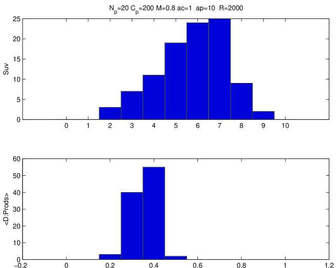
Figure 7: Instability of the producer selection process. The histogram of the number of surviving producers, the upper diagram, displays a strong reduction from initial producer number, $N_{p}=100$, with large deviations. The lower histogram displays distances among producer strings, and shows that they are concentrated in only a small part the hypercube.

The initial dynamics of accumulation of customers in the satisfaction basin of the survivors displayed on figure 8 comfort our hypotheses. One observes a strong population increase in the satisfaction basin of the surviving producers and a slow decay in the neighborhood of the opposite strings. The random initial population of any 2-neighbourhood is 56 on average.

The two growth regimes, fast initial increase and slower later increase are understandable: the initial population increase (during the first 100 time steps) is due to the fact that any site on the 2-neighbourhood of a surviver has a much longer lifetime than those in the desert (the desert time life=5). Close to the producers the life time is infinite at 0 distance, 50 at distance 1, 25 at distance 2. Re-born consumers (1/5) have a 1000/56 chance to get to an attraction basin of a surviver, which gives the observed figure of 100 time steps for the steep increase duration. Later the slow growth correspond to the replacement of consumers in the attraction basin by those who hit the surviver site and thus eternity.

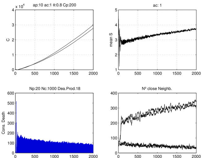
Figure 8: Time evolution of producers capital $C_{i}$, of the average consumer satisfaction $S$, of the number of consumer death per time unit and of the number of customers in the attraction basin of the two surviving producers (rising curves) and of two random sites. $N_{p}$ initial was 20,$N_{c}=1000$, $a_{c}=1$, $\theta=1$. But the value of $a_{p}=10$ gives rise to a strong selection of producers.

5 Conclusions

The present version of the model is evidently very crude with respect to the more general aspects than one would like to investigate in this framework. One would like to better understand the dynamics of co-evolution when producers are endowed with stategic behaviour. This line of research has already been investigated by [9]. We can predict from our present study that producers strategies may be influential and provide higher gains in the competition regime. When the niche regime is established their efficiency will be extremely limited because of the condensation of consumers in the neighbourhood of producers. Other renewal processes can be imagined for consumers such as myopic learning or reproduction with noise (with probably equivalent results in the two latter cases).

In other words, the present study has set the stage for more intricate studies in co-evolution.

Acknowledgments: The first author (TA) thanks R. Vilela Mendes for the illuminating discussions on the original model. The present work was started on the occasion of Gérard Weisbuch visit to Lisbon, supported by FCT-Portugal, grant PDCT/EGE/60193/2004. GW was also supported by E2C2 NEST 012410 EC grant.

References

- [1] P.W. Anderson; Suggested model of prebiotic evolution: The use of chaos, Proc. Nat. Acad. Sci. U.S.A., 80 (1983), 3386-3390.
- [2] J.D. Farmer, N.H. Packard, A.S. Perelson; The immune system, adaptation, and machine learning, Physica D, (1986), 187-204.
- [3] L. Riolo, Rick, Cohen, D. Michael, R. Axelrod, ; Evolution of cooperation without reciprocity, Nature, v. 414, (2001), 441-443.
- [4] R. Axelrod; The Dissemination of Culture: A Model with Local Convergence and Global Polarization , Journal of Conflict Resolution, (1997).
- [5] G. Weisbuch, G. Deffuant, F. Amblard, J-P. Nadal; Meet, discuss, and segregate!, Complexity, v.7, 3, (2002), 55-63.
- [6] D. Challet, Y-C. Zhang; On the Minority Game: Analytical and Numerical Studies, (1998), arXiv:cond-mat/9805084.
- [7] J. H. Holland and J. S. Reitman; Cognitive systems based on adaptive algorithms, ACM SIGART Bulletin archive, 63, ACM Press New York, 1977.
- [8] E. Berne; What do you say after you say hello? : the psychology of human destiny, Bantam, New York, 1981.
- [9] T. Araujo and R. Vilela Mendes; Market-oriented innovation: When is it profitable? An abstract agent-based study,WP31/2006/DE/UECE,(2006).