Dynamical thermal response functions for strongly correlated one-dimensional systems

Abstract

In this article we study the thermal response functions for two one-dimensional models, namely the Hubbard and spin-less fermion $t$-$V$ models. By exactly diagonalizing finite sized systems we calculate dynamical electrical, thermoelectrical, and thermal conductivities via the Kubo formalism. The thermopower (Seebeck coefficient), Lorenz number, and dimensionless figure of merit are then constructed which are quantities of great interest to the physics community both theoretically and experimentally. We also geometrically frustrate these systems and destroy integrability by the inclusion of a second neighbor hop. These frustrated systems are shown to have enhanced thermopower and Lorenz number at intermediate and low temperatures.

I Introduction

Strongly correlated electron systems are currently at the forefront of physics. These systems provide some of the most interesting theoretical challenges and many experimental systems of fundamental and technological interest consist of strongly correlated constituent particlesTokura (2003); Imada et al. (1998). It is at the convergence of the fundamental and the technological that thermal response functions of strongly correlated systems take on particular importance. This is certainly true in the high thermopower material sodium cobalt oxideLevi (2003); Terasaki et al. (1997); Wang et al. (2003); Haerter et al. (2006) as well as other transition metal oxides such as the high $T_{c}$ superconductors. Thermal behavior is also of interest in experimental one-dimensional systems such as carbon nanotubesHone et al. (1998), semiconductor nanowiresZhou et al. (2006), and organic compoundsEpstein et al. (1979); Kwak et al. (1976), to name a few.

One-dimensional systems are very interesting from the point of view of the exotic collective behavior of excitations due to reduced dimensionality. This is manifested most strikingly in the existence of a Luttinger liquid of bosonic excitations in generic 1D systems at low temperatures. Electrical and thermal transport in these systems is of great interestKane and Fisher (1996). One-dimension also allows the existence of a class of systems known as integrable systems, where there is an infinite family of commuting operators that commute with the HamiltonianShastry (1986); Yang and Yang (1966); Sutherland (2004). Recently, Shastry Shastry (2006a, b, 2007) has introduced a high frequency formalism for thermoelectrics (discussed below) that is particularly suited for strongly correlated electron systems. Hence, one-dimensional systems provide good systems in which to benchmark his new high frequency formalism.

Geometrical frustrationRamirez (2001) has generated much interest in the physics community throughout past decades. Recently it has been shown that strong electron correlations in conjunction with the geometrical frustration induced by a two-dimensional triangular lattice are the keys to understanding the Curie-Weiss metallic phase in sodium cobalt oxideHaerter et al. (2006). Geometrical and/or electrical frustration is also the key to the emergence of kinetic anti-ferromagnetismHaerter and Shastry (2005), and to a description of quantum spin glassesRamirez (2001).

In a one-dimensional system it is possible to induce frustration by considering kinetic energy hoppings further than nearest neighbors, i.e., second nearest neighbors. We demonstrate in this paper that frustration of this sort also has very interesting effects on transport properties in addition to the equilibrium properties alluded to above. One such effect is enhancement of the thermopower compared to the unfrustrated system recently predicted by Shastry Shastry (2006a, b, 2007); Haerter et al. (2006). Understanding this enhancement could lead to clues towards the creation, in material science laboratories, of custom made high thermopower materials with far reaching consequences to the scientific community.

Theoretically, strongly correlated systems are notoriously difficult due in part to the fact that perturbation theory is not applicable. For dynamical thermal response functions (using the Kubo Kubo (1957) formalism), knowledge of the full eigenspectrum is necessary, therefore, progress is made via exact diagonalization of finite sized systems. The models and systems we study are the Hubbard and spin-less fermion $t$-$V$ model on one-dimensional rings (periodic boundary conditions) of up to $\mathcal{L}=10$ sites for the Hubbard model and $\mathcal{L}=16$ sites for the spin-less fermion $t$-$V$ model. Newer theoretical methods are constantly being developed, such as the dynamical mean field theoryKotliar and Vollhardt (2004); Georges et al. (1996), finite temperature Lanczos (FTL) methodsJaklic and Prelovsek (2000), cluster perturbation theoryMaier et al. (2005), etc.. In fact, the dynamical mean field theory approximation has considered some thermoelectric variables previously, although in a limited range of model parameter space, c.f. Ref. Oudovenko and Kotliar, 2002 and Pálsson and Kotliar, 1998. It is important, as a first step, to approach these systems with a rigorously exact method (exact diagonalization) to, if nothing else, provide a benchmark for further approximate studies and methods. Of course, there are obvious shortcomings to exact diagonalization, i.e., finite size effects due to the smallness of the system and the computational price is often quite expensive. However, we find only the very low temperature regimes ($T<1|t|$) troublesome in our studies which, incidentally, are the regimes that other approximations also have difficulty tackling. Interestingly, the high frequency formalism of Shastry, compared to dynamical approximations, is significantly less expensive computationally and perhaps could lend itself even more profitably to new and existing approximate methods.

We primarily use the Hubbard model for our studies and carry out the most extensive calculations on it. The $t$-$V$ model is mainly used to supplement the study of the Hubbard model, partly due to the fact that some of the transport coefficients turn out to be identically zero in this model as discussed in Sec. IV.2 and partly because the calculation of some of the operators are very involved, owing to the interaction being between neighboring sites and not on-site. The numerical calculation of the thermopower is the most tractable and is performed extensively. The calculations presented here are the first detailed calculations (considering the full range of model parameter space) in the literature for the thermopower, Lorenz number, and dimensionless figure of merit for strongly correlated models.

The plan of this paper is as follows: in section II we introduce the models to be studied and provide an overview of our exact diagonalization procedure. Section III reviews the Kubo formalism for the thermoelectric conductivities needed to calculate the physical observables of interest. Section IV, V, and VI present results for the thermopower, Lorenz number and thermoelectric figure of merit (FOM), respectively, for the models we study. We present our conclusions and a summary in section VII.

II Models

The Hubbard model is described by a Hamiltonian with a kinetic energy term which allows electrons to hop between sites $j$ and $j+\eta$ with probability $t(\eta)$ and an on-site electron repulsion potential energy governed by parameter $U$, i.e.,

$$\hat{H} = -\sum_{j=1}^{\mathcal{L}}\sum_{\eta=1}^{2}\sum_{\sigma}t(\eta)\{\hat{c}^{\dagger}_{j+\eta\sigma}\hat{c}_{j\sigma}+{\rm h.c.}\}$$ (1)

$$+U\sum_{j=1}^{\mathcal{L}}(\hat{n}_{j\uparrow}-1/2)(\hat{n}_{j\downarrow}-1/2)\;,$$

where $\hat{c}^{\dagger}_{j\sigma}(\hat{c}_{j\sigma})$ create(destroys) an electron with spin $\sigma=(\uparrow,\downarrow)$ at the lattice site $j$, $\hat{n}_{j\sigma}=\hat{c}^{\dagger}_{j\sigma}\hat{c}_{j\sigma}$ is the number operator, and $\eta=1$ and $\eta=2$ for first and second nearest neighbor hoppings, respectively. The electron operators obey the usual anti-commutation rules $\{\hat{c}_{j\sigma},\hat{c}^{\dagger}_{j^{\prime}\sigma^{\prime}}\}=\delta_{jj^{\prime}}\delta_{\sigma\sigma^{\prime}}$. We assume $t(1)=t$, $t(2)=t^{\prime}$, and $t(\eta)=0$ for all other $\eta$. With $t^{\prime}=0$, this Hamiltonian is particle-hole symmetric as can be seen from the local transformation $\hat{d}_{j\sigma}^{\dagger}=(-1)^{j}\hat{c}_{j\sigma}$. This transformation leaves $t$ and $U$ invariant, while taking $N_{\sigma}\rightarrow 1-N_{\sigma}$, where $N_{\sigma}$ is the total number of electrons with spin $\sigma$ and the total number of electrons is $N=\sum_{\sigma}N_{\sigma}$. Since it takes $t^{\prime}\rightarrow-t^{\prime}$, a non-zero $t^{\prime}$ breaks particle-hole symmetry. Even in the presence of $t^{\prime}\neq 0$, this transformation is useful since it tells us that a quantity $A(N_{\uparrow},N_{\downarrow},t,t^{\prime},U)=\pm A(\mathcal{L}-N_{\uparrow},\mathcal{L}-N_{\downarrow},t,-t^{\prime},U)$. Thus knowing the value of $A$ up to half-filling for $t^{\prime}$ and $-t^{\prime}$ lets us construct the entire dependence on filling in both cases, provided we know whether $A$ is odd or even under the particle-hole transformation. We only consider electron repulsion $U>0$ and assume periodic boundary conditions (one-dimensional rings).

The spin-less fermion $t$-$V$ models is governed by a Hamiltonian with a kinetic energy term similar to the Hubbard model (without the spin) but the potential energy describes a nearest neighbor repulsion governed by a parameter $V$, i.e.,

$$\hat{H} = -\sum_{j=1}^{\mathcal{L}}\sum_{\eta=1}^{2}t(\eta)\{\hat{c}^{\dagger}_{j+\eta}\hat{c}_{j}+{\rm h.c.}\}$$ (2)

$$+V\sum_{j=1}^{\mathcal{L}}(\hat{n}_{j}-1/2)(\hat{n}_{j+1}-1/2)\;.$$

Like the Hubbard model we assume here that $t(1)=t$, $t(2)=t^{\prime}$ and $t(\eta)=0$ for all other $\eta$ and $V>0$. This model too has the same particle-hole symmetry but without the spin. Once again, $t^{\prime}$ breaks the particle-hole symmetry and a calculation up to half-filling (with $t^{\prime}>0$ and $t^{\prime}<0$) lets us extrapolate to all values of filling.

As with any exact diagonalization there exist computational limitations due to the obvious difficulties in dealing with large matrices. In view of these limitationscl- the Hubbard model is computed for $N=$1,$\ldots$,5 and 5,$\ldots$,8 electrons on $\mathcal{L}=$10 and 8 site systems, respectively. These particular systems correspond to electron fillings (densities) of $n=N/\mathcal{L}=$0.1, 0.2, 0.3, 0.4, 0.5, 0.625, 0.75, 0.875, and 1. The $t$-$V$ model allows a larger lattice size stemming from the lack of the spin degree of freedom and we present data for $L=16$ (and $N=1,\ldots,8$). The large Hilbert spaces can be reduced by considering systems with a constant $z$-component of spin (for the Hubbard model). The sector with the smallest $z$-component of spin has the largest Hilbert subspace dimension and dominates the physics. Linear momentum is a good quantum number due to the translational invariance of our systems and we implement this symmetry to further reduce the Hilbert space to more manageable proportions. However, we point out that the bottleneck of our calculations is not necessarily the Hamiltonian diagonalization but the finite temperature averages of certain operators and evaluation of the full Kubo formulas discussed below.

The density of states of our models for $t^{\prime}=0$ has two van Hove singularities at the band edges. If $|t^{\prime}|>0.25|t|$ another singularity is introduced which will invariably produce large changes in the thermoelectric properties. However, we are interested here in the more subtle effects arising from geometrical frustration and strong interactions, hence, by introducing a non-zero $|t^{\prime}|<0.25|t|$ the density of states maintains only the original two van Hove singularities.

In order to display effects of electron correlations the interaction parameter $U(V)$ must be at least a few times larger than the bandwidth which is equal to $W=4|t|$ for both models. We consider three values of interaction strength for each model corresponding roughly to the non-interacting case where the interaction parameter is equal to zero ($U(V)=0\ll W$), the weakly interacting case where the interaction is equal to roughly the bandwidth ($U(V)\sim W$), and the strongly interacting case where the interaction is a few times greater than the bandwidth ($U(V)\gg W$).

III Dynamical thermal response functions

Conductivities are computed via the Kubo linear response formalismMahan (1990) recently presented in detail by Peterson et al in Ref. Peterson et al., 2007 which closely followed the work of ShastryShastry (2006a, b, 2007). In particular, we calculate the Kubo formulas for the electrical $\sigma(\omega)$, thermoelectrical $\gamma(\omega)$, and the thermal $\kappa(\omega)$ conductivities, respectively, which then allows us to calculate physical quantities of interest such as the thermopower $S$ (or Seebeck coefficient), the Lorenz number $L$, and the dimensionless figure of merit $ZT$, given as

$$S(\omega,T)=\frac{\gamma(\omega,T)}{\sigma(\omega,T)}\;,$$ (3)

$$L(\omega,T)=\frac{\kappa(\omega,T)}{T\sigma(\omega,T)}-S(\omega,T)^{2}\;,$$ (4)

and

$$Z(\omega,T)T=\frac{S(\omega,T)^{2}}{L(\omega,T)}$$ (5)

given here for completeness and ease of presentation. The second term in Eq. 4 is produced by the zero electric current constraint under a thermal gradientZiman (1979). This term is usually small (especially at low temperatures) for metals and semiconductors and often ignored. However, as will be shown, for strongly correlated lattice systems like those studied here, this term is an important actor especially at high temperatures.

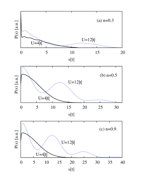
Figure 1: Probability density of states $P(s)$ with energy difference $s=|\varepsilon_{i}-\varepsilon_{j}|$. The solid black and dashed blue lines represent $U=4|t|$ and $12|t|$, respectively, for density $n=0.3$ (a), $n=0.5$ (b), and $n=0.9$ (c). The position of the maximum probability for the lower Hubbard band is insensitive to the value of $U$.

However, one is usually interested in the DC ($\omega\rightarrow 0$) limit of the dynamical conductivities. For finite sized systems this requires the introduction of a level broadening $\epsilon$ which smoothens the divergences caused by the discrete nature of the eigenspectrum. Often $\epsilon$ is taken to be equal to the mean energy level spacing of the system which is of order $\mathcal{O}(|t|/\mathcal{L})$. However, for the Hubbard model, as the interaction energy $U$ is increased the mean energy level spacing begins to include upper Hubbard bands. In Fig. 1(a)-(c) the probability density of states $P(s)$ with energy difference $s=|\varepsilon_{i}-\varepsilon_{j}|$ ($\varepsilon_{k}$ is the eigenenergy of state $k$) is plotted for three representative cases, namely, fillings $n=0.3$, $0.5$, and $0.9$, for $U=4|t|$ (weakly-coupled) and $U=12|t|$ (strongly-coupled).

It is clear from Fig. 1(a)-(c) that the most probable energy difference between states in the lower Hubbard band is relatively immune to changes in either filling or interaction strength. However, the appearance of the upper Hubbard bands in the strongly-coupled case yields an $\epsilon$ that is very large (compared to the bandwidth) and strongly $U$ dependent. The large $U$ situation yields a large $\epsilon$ which tends to mask real physical contributions to the current matrix elements coming from transitions between Hubbard bands. Therefore, in this work we choose $\epsilon$ to be approximately equal to the mean energy level spacing in the lower Hubbard band for all cases, i.e., $\epsilon=0.8|t|$ for the Hubbard modeleps .

As discussed previously in detail in Ref. Peterson et al., 2007 another frequency limit, besides the DC limit, is the infinite frequency limit which is defined as (for completeness)

$$S^{*}(T)=\lim_{\omega\rightarrow\infty}S(\omega,T)=\frac{\langle\hat{\Phi}_{xx}\rangle}{T\langle\hat{\tau}_{xx}\rangle}\;,$$ (6)

$$L^{*}(T)=\lim_{\omega\rightarrow\infty}L(\omega,T)=\frac{\langle\hat{\Theta}_{xx}\rangle}{T^{2}\langle\hat{\tau}_{xx}\rangle}-[S^{*}(T)]^{2}\;,$$ (7)

and

$$Z^{*}(T)T=\lim_{\omega\rightarrow\infty}Z(\omega,T)T=\frac{[S^{*}(T)]^{2}}{L^{*}(T)}\;.$$ (8)

with the operators $\hat{\tau}_{xx}$, $\hat{\Phi}_{xx}$, and $\hat{\Theta}_{xx}$ defined in Shastry (2006a, b, 2007). These quantities can be calculated as equilibrium expectation values of operators that, while non-trivial, are easier to calculate and less time consuming numerically than the full dynamical quantities via the Kubo formulas. All of the interaction effects remain in these quantities but, importantly, the dynamics have been separated from the interactions.

IV Thermopower

The thermopower, or Seebeck coefficient, is defined as the ratio of the thermoelectrical to the electrical conductivity and measures the electrical response of a material to a temperature gradient. Like the Hall coefficient it is often assumed to measure the sign of the charge carriers in a particular material.

The thermopower $S(\omega,T)$ can be instructively rewrittenHaerter et al. (2006); Peterson et al. (2007), by isolating the term containing the chemical potential $\mu(T)$, as

$$S(\omega,T)=S_{tr}(\omega,T)+S_{MH}(T)$$ (9)

The first term is due to electrical transport while the second is entropic in origin and is the familiar Mott-HeikesChaikin and Beni (1976) term $S_{MH}(T)=-(\mu(T)-\mu(0))/q_{e}T$. These two terms both contribute to the thermopower in different and often competing ways.

Strongly correlated systems are difficult to make theoretical progress on and the first term in Eq. 9 is usually the most intractable. For many systems this term is small (especially at low temperatures), compared to the second term, and fruitfully ignored. In this approximation the thermopower is dominated by the Mott-Heikes (MH) term. The MH limit is described as the limit when $k_{B}T\gg|t|$. This limit is achieved at either very high temperatures or at more modest temperatures in narrow band systemsChaikin and Beni (1976). The usefulness of the MH term is that at high temperatures the chemical potential is linear in $T$ leaving the MH limit constant. Even though the MH limit is constant it contains a non-trivial filing dependence that arises from the particular nature of the Hilbert space. Many of these MH limits were considered previouslyChaikin and Beni (1976) and below we quote them for the spin-less fermion $t$-$V$ model for finite and infinite $V$ in Eq. 13. As will be shown below, the transport term (first term in Eq. 9) is very important for low to intermediate temperatures and the MH term alone is clearly inadequate in this temperature regime.

The thermopower is expected to vanish in the zero temperature limit. This is physically intuitive and has been shown theoretically for the one-dimensional Hubbard model via a version of the Bethe ansatz solutionStafford (1993). In our formalism this $T=0$ vanishing is accomplished through a subtle balance of the transport and MH terms as $T\rightarrow 0$. For thermodynamically large systems this balance is obtained. However, for finite systems, even in the non-interacting limit, the balance is not manifest resulting in thermopower divergences as $T\rightarrow 0$ due to finite size effects.

This balance suggests a rewriting of the thermopower, given in Ref. Haerter et al., 2006; Peterson et al., 2007, in such a way to ensure that the thermopower vanishes at $T=0$ by forcing both the transport ($S_{tr}(\omega,T)$) and MH ($S_{MH}(T)$) terms to independently vanish in that limit. This rewriting yields a frequency dependent transport term and the frequency independent MH term.

Finite sized systems have a few more subtleties which we now describe. The chemical potential is commonly defined as $\mu(T)=\partial F_{N}(T)/\partial N$, where $F_{N}(T)$ is the Helmholtz free energy for an $N$ particle system. For our finite systems we will approximate this partial derivative as $\mu(T)=(F_{N+1}(T)-F_{N-1}(T))/2$ for $N\geq 2$ or $\mu(T)=F_{N+1}(T)-F_{N}(T)$ for $N=1$ since there is no system for $N=0$. As discussed in Ref. Peterson et al., 2007 the ground state degeneracy of a system (if it exists) is discounted when calculating $\mu(T)$ so as to eliminate a leading order term linear in $T$ that produces a non-zero $S_{MH}(T)$ as $T\rightarrow 0$. Further, finite systems have discrete energy levels giving rise to an energy gap. The energy gap causes an exponential behavior in $\mu(T)$ which is not a serious problem since it vanishes faster than $T^{2}$. Both of these particulars, however, create a chemical potential which does not behave as $T^{2}$ at low $T$ as expected for thermodynamically large systems.

In the following figures the thermopower will be given in its “natural” units of $k_{B}/q_{e}$ where $q_{e}=-|e|$ with $|e|$ the value of the electron charge. For experimental comparison one simply replaces $k_{B}/|e|=86\mu V/K$.

IV.1 Hubbard model

The MH term is the high temperature limit $k_{B}T\gg|t|$ of $S_{MH}(T)$. As discussed elsewhereChaikin and Beni (1976); Peterson et al. (2007) the MH limit of the finite $U$ situation is essentially the uncorrelated band since the temperature is necessarily much larger than $U$. To understand the effects strong interactions play (large $U$) one must consider infinite $U$ when calculating this limit.

In the finite $U$ case, the MH limit has a single zero crossing at half filling $n=1$ where the thermopower is seen to change sign and it diverges in the band-insulator limits ($n=0$ and $n=2$). For the infinite $U$ case there are two additional zero crossings and one additional divergence. The MH limit still diverges in the band-insulator limits but now also diverges for the Mott insulator ($n=1$). The two additional sign changes occur for fillings $n=2/3$ and $n=4/3$. The MH limit in the infinite $U$ case for $n\geq 1$ is found from the MH limit for $0\geq n\geq 1$ through particle-hole symmetry ($n\rightarrow 2-n$ and $q_{e}\rightarrow-q_{e}$). There is no $t^{\prime}$ dependence for the MH limits, therefore, they lead to the conclusion (for $t$ and $t^{\prime}$) that the Hubbard model should have interaction induced sign changes of the thermopower at $n\approx 2/3$ (and $n\approx 4/3$ using particle-hole symmetry).

(a)

(b)

(c)

Figure 2: (color online) $S^{*}(T)$ (black line) as a function of filling $n$ and temperature $T$. For (b) and (c) the orange dotted lines are the DC limit $S(0,T)$ of the full thermopower for comparison. Projected onto the $T=5|t|$ plane are the MH limits for both the finite (red line) and infinite $U$ (blue dashed line) situations.

(a)

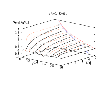
(b)

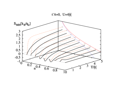
(c)

Figure 3: (color online) $S_{MH}(T)$ (black line) as a function of filling $n$ and temperature $T$. For (b) and (c) the orange dotted lines are the infinite frequency limit $S^{*}(T)$ for comparison. Projected onto the $T=5|t|$ plane are the MH limits for both the finite (red line) and infinite $U$ (blue dotted line) cases.

First we consider results for the one-dimensional Hubbard model with $t^{\prime}=0$.

IV.1.1 Hubbard with $t^{\prime}=0$

Here we consider the Hubbard model with $t^{\prime}=0$ in the non-interacting ($U=0$), the weakly correlated ($U=4|t|$), and the strongly correlated ($U=12|t|$) cases, respectively.

Due to the particle-hole symmetry of the $t^{\prime}=0$ Hubbard model $\mu(T)$ for $N=\mathcal{L}$ is

$$\mu(T) = \frac{1}{2\beta}\ln\left(\frac{\mathcal{Z}_{\mathcal{L}-1}}{\mathcal{Z}_{\mathcal{L}+1}}\right)$$ (10)

$$= \frac{1}{2\beta}\ln\left(\frac{\mathcal{Z}_{\mathcal{L}-1}}{e^{-\beta U}\mathcal{Z}_{\mathcal{L}-1}}\right)=\frac{U}{2}$$

since an energy eigenstate for $N$ electrons and $2\mathcal{L}-N$ electrons are related through $\varepsilon_{k}(N)=\varepsilon_{k}(2\mathcal{L}-N)-(\mathcal{L}-N)U$ according to Lieb and WuLieb and Wu (1968). Hence, $S_{MH}(T)$ is identically zero for all $T$. The transport term $S_{tr}(T)$ is also identically zero for all $T$ due to particle-hole symmetry and hence we find that $S(\omega,T)=0$ for $n=1$ for all $T$ and $\omega$. This argument equally applies to the spin-less $t$-$V$ model for $t^{\prime}=0$.

In Fig. 2(a)-(c) we plot the infinite frequency limit of the thermopower $S^{*}(T)$ and the DC limit ($\omega\rightarrow 0$) of the full Kubo thermopower $S(\omega,T)$ versus temperature $T$ and filling $n$ for $U=0|t|$ (a), 4$|t|$ (b), and 12$|t|$ (c). Projected onto the the $T=5|t|$ plane are the MH limits for finite and infinite $U$ scenarios.

For the non-interacting case in Fig 2(a) there is no frequency dependence as both the charge and heat current operators are diagonal. The thermopower grows monotonically and, essentially, linearly from zero at $T=0$ to the MH limitmh- near $T=5|t|$. As the temperature is increased the slope of the linear regime is lessened and the thermopower approaches the MH limit more slowly. Some finite size effects are evident at the largest fillings $n=$6/8 and 7/8 calculated where some somewhat strange low temperature effects are observed.

The effect of interactions shown in Fig. 2(b)-(c) is to generally reduce the thermopower for fillings greater than $n=2/3$. For fillings below $n\sim 0.625$ the DC and infinite frequency thermopower are essentially identical. At fillings greater than $n=0.625$ $S(0,T)$ and $S^{*}(T)$ display slight differences at low temperatures for the weakly correlated regime ($U=4|t|$, Fig. 2(b)) and marked differences for the strongly interacting regime ($U=12|t|$, Fig. 2(c)).

The thermopower at half filling in all cases is pinned at zero as discussed. For $n=0.875$ the effect of interactions is to reduce the thermopower (Fig 2(b)), changing its sign (Fig. 2(c)), for low to intermediate temperatures. Eventually the entropy dominates and the thermopower begins to climb towards its entropy determined MH limit. It should be noted that even for the highest temperature $T=5|t|$ the thermopower remains negative for $n=0.875$ and $U=12|t|$.

In Fig. 3(a)-(c) we plot the MH term of the thermopower ($S_{MH}(T)$) versus temperature and filling for $U=0$, $4|t|$, and $12|t|$, respectively. Also shown is $S^{*}(T)$ for comparison. Interestingly, the transport term increases the low to mid temperature thermopower for all fillings in the non-interacting and weakly interacting cases. For the strongly interacting case in Fig. 3(c) the transport term begins to decrease the thermopower at low temperatures and high fillings ($n\geq 0.75$).

The results in this section can be directly compared with Ref. Zemljic and Prelovsek, 2005 which used the FTL method which allowed rings of up to $\mathcal{L}=14$ sites. Their results were for a much lower window of temperatures $0.2|t|<T<2|t|$ and show a greater thermopower suppression for more modest values of $U$ than in the present work. The thermopower in the low temperature regime is very sensitive to any changes in either the $S_{tr}(T)$ or $S_{MH}(T)$. Considering that Ref. Zemljic and Prelovsek, 2005 used a larger system but an approximation it is unclear as to the nature of the discrepancy between those results and the present study. However, the qualitative behavior of both calculations is consistent.

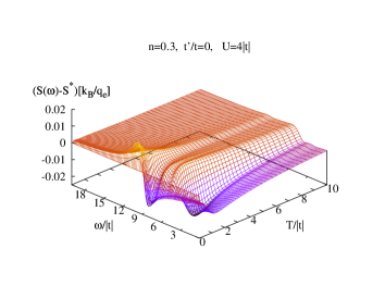
(a)	(b)
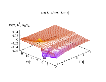
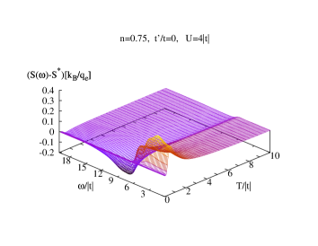
(c)	(d)
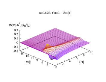
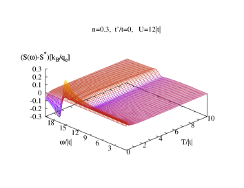
(e)	(f)
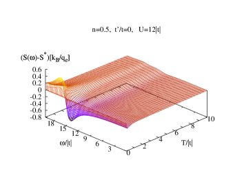
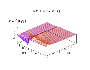
(g)	(h)

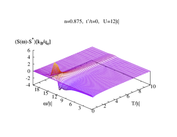
Figure 4: (color online) $S(\omega,T)-S^{*}(T)$ as a function of frequency $\omega$ and temperature $T$ for the weak coupling case $U=4|t|$, $t^{\prime}=0$, and fillings (a) $n=0.3$, (b) $n=0.5$, (c) $n=0.75$, and (d) $n=0.875$. Panels (e)-(h) represent the strong coupling case $U=12|t|$ for the same fillings as the weak coupling case. The main frequency dependence occurs near $\omega\sim U$ for low to intermediate temperatures. The largest frequency dependence near $T=0$ is likely a finite size effect. There is no frequency dependence for the half filled case $n=1$ (not shown).

Next the full frequency and temperature dependence of the thermopower is investigated. Fig. 4(a)-(h) plots the difference in the full frequency dependent thermopower minus the infinite frequency limit, i.e., $S(\omega,T)-S^{*}(T)$. For the weak coupling (Fig. 4(a)-(d)) case there is little frequency dependence except for when $\omega\sim U$ at low to intermediate temperatures. In what is surely a consequence of the finite sized system there appears to be an even/odd effect in that for even numbers of electrons (Fig 4(c) and not shown) $S(\omega,T)-S^{*}(T)$ is positive for $\omega<U$ and negative for $\omega>U$ while for odd numbers of electrons (Fig 4(a)-(b)-(d)) the opposite effect is observed. Of course, for half filling there is no frequency dependence (not shown).

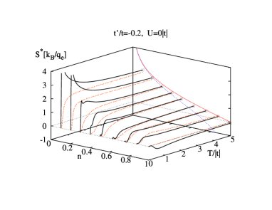
(a)	(b)
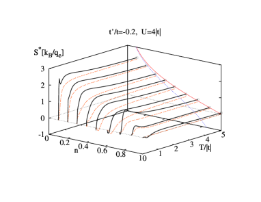
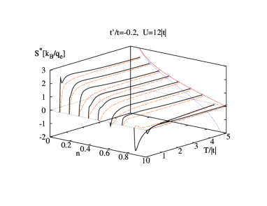
(c)	(d)

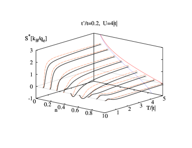
Figure 5: (color online) $S^{*}(T)$ (black line) as a function of filling $n$ and temperature $T$ for (a) $U=0$, (b) $U=4|t|$, and (c) $U=12|t|$ and $t^{\prime}/t=-02$.. The full $S(\omega,T)$ (not shownt (02)) compares similarly to $S^{*}(T)$ for $t^{\prime}\neq 0$ as for $t^{\prime}=0$, c.f. Fig. 4. The red curve is for $t^{\prime}=0$ to facilitate an easy comparison. As an example of the other sign of $t^{\prime}$, namely, $t^{\prime}/t=0.2$, (d) shows the expected reduction in $S^{*}(T)$ for $U=4|t|$ (similar results obtained for $U=0$ and $U=12|t|$ are not shown). The MH limits are projected unto the $T=5|t|$ plane for finite $U$ (red line) and infinite $U$ (blue dotted line).

The same qualitative behavior is found for the strongly correlated regime in Fig. 4(e)-(h). Again the even/odd effect is obtained (cf. Fig. 4(g) vs. Fig. 4(e), (f), and (h)) and the frequency dependence is generally weak except for $\omega\sim U$. The main difference between the $U=12|t|$ and the $U=4|t|$ cases is that the frequency dependence at $\omega\sim U$ in the former is larger. It should be kept in mind that the largest frequency dependences occur for the lowest temperatures and the thermopower for a finite sized system in the low temperature regime is susceptible to finite sized effects that could possibly not survive in the thermodynamic limit. Therefore, it is safe to assume that our results are qualitatively representative of a thermodynamically large Hubbard model but perhaps not quantitatively accurate.

Similar qualitative frequency dependence was seen in Ref. Zemljic and Prelovsek, 2005 for a low temperature slice ($T=0.5|t|$) and high fillings ($n>0.7$). The difference in that work and the present work is that the frequency dependence occurred nearer to $\omega\sim U/2$ in the former where in the present result the largest frequency dependence occurs near $\omega\gtrsim U$.

Unless one is concerned with extremely low temperatures and frequencies similar in magnitude to the interaction strength $U$ the infinite frequency thermopower $S^{*}(T)$ is a good representative of the full thermopower $S(\omega,T)$. Recently, a similar calculation on the strongly correlated $t$-$J$ model for a two-dimensional triangular lattice was carried out in Ref. Peterson et al., 2007 where it was found that the frequency dependence was much weaker justifying the use of $S^{*}(T)$ in place of $S(\omega,T)$.

IV.1.2 Hubbard with $t^{\prime}\neq 0$

Here we investigate the effect of frustration on the thermopower by considering the case of a non-zero second neighbor hopping amplitude $|t^{\prime}|/t=0.2$.

Recently, Shastry Shastry (2006a, b, 2007) predicted a low to intermediate temperature enhancement of the thermopower via a high temperature expansion of the high frequency limit $S^{*}(T)$ for the geometrically frustrated two-dimensional triangular lattice $t$-$J$ model. In that case, changing the sign of the hopping was found to enhance the thermopower at intermediate temperatures. Haerter et. al.Haerter et al. (2006) and Ref. Peterson et al., 2007 more thoroughly investigated that particular case.

In one-dimension it is similarly expected that an enhancement of the thermopower will occur when a second-neighbor hop is added to the kinetic energy which frustrates the lattice and destroys integrability.

Fig. 5(a)-(d) show $S^{*}(T)$ versus temperature and filling for values of $t^{\prime}/t=-0.2$ (Fig. 5(a)-(c)) and $t^{\prime}/t=0.2$ (Fig. 5(d)). For this case we do not plot the full frequency dependence but remark that it is similar qualitatively and quantitatively to the $t^{\prime}=0$ caset (02).

When $t>0$ and $t^{\prime}<0$ the thermopower is enhanced at low temperatures. The enhancement is seen to arise from almost purely the transport term of the thermopower (first term in Eq. 9). Fig. 6 shows $S^{*}(T)$ and the MH term $S_{MH}(T)$ for $t^{\prime}/t=-0.2$ and $U=4|t|$ as a representative example. Similar to the results displayed in Fig. 3 the low temperature thermopower is dominated by the transport term and in the case of $t^{\prime}/t=-0.2$ that domination is even more pronounced as it produces an enhancement peak.

For small fillings the enhancement has weak $U$ dependence although the non-interacting case seems to be tending to diverge at very low temperatures ($n=0.1$ and $n=0.2$ in Fig. 5(a)) that is most certainly a finite size artifact. At fillings above $n=0.5$ there are interaction effects which are visible at low temperatures. For the frustrated case discussed here the thermopower still mostly achieves its MH limit by $T=5|t|$ as expected.

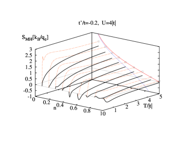
Figure 6: (color online) $S_{MH}(T)$ (black line) as a function of filling $n$ and temperature $T$. The orange dotted lines are the infinite frequency limit $S^{*}(T)$ for comparison. Projected onto the $T=5|t|$ plane are the MH limits for both the finite (red line) and infinite $U$ (blue dotted line) cases.

For the situation when $t$ and $t^{\prime}$ are both positive there is a suppression of the thermopower at low temperatures, c.f. Fig. 5(d), hence the opposite effect. Only the weakly correlated $U=4|t|$ case is plotted to illustrate this.

For both signs of $t^{\prime}$ at half filling ($n=1$) the thermopower is no longer identically zero since the addition of a non-zero $t^{\prime}$ destroys the particle-hole symmetry, however, the thermopower remains quite small at this density.

IV.2 $t$-$V$ model

(a)

(b)

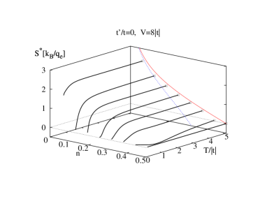
(c)

Figure 7: (color online) $S^{*}(T)$ (black line) as a function of filling $n$ and temperature $T$. For (b) and (c) the orange dotted lines are the DC limit $S(0,T)$ of the full thermopower for comparison. Projected onto the $T=5|t|$ plane are the MH limits for both the finite (red line) and infinite $V$ (blue dotted lines) situations.

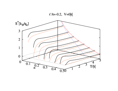
(a)	(b)
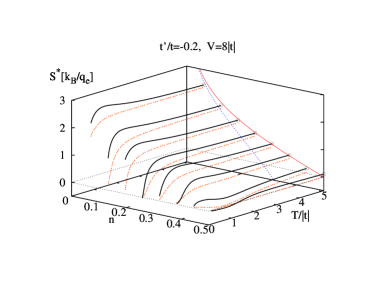
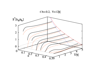
(c)	(d)

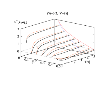
Figure 8: (color online) $S^{*}(T)$ as a function of filling $n$ and temperature $T$ for (a) $V=0$, (b) $V=8|t|$, and (c) $V=12|t|$. The full $S(\omega,T)$ compares similarly to $S^{*}(T)$ as for the $t^{\prime}=0$ case, c.f. Fig. 4. The red curve is $S^{*}(T)$ for $t^{\prime}=0$ to facilitate an easy comparison. As an example of the other sign of $t^{\prime}$, namely, $t^{\prime}/t=0.2$, (d) shows the expected reduction in $S^{*}(T)$ for $V=8|t|$. The MH limits are projected unto the $T=5|t|$ plane for finite $V$ (red line) and infinite $V$ (blue dotted line).

Most of the considerations of the thermopower for the Hubbard model also apply to the $t$-$V$ model. In particular this model too has particle hole symmetry at half-filling ($n=0.5$ instead of $n=1$ as for the Hubbard model, since the spin degree of freedom is absent) and thus the thermopower is identically zero at all temperatures. The thermopower is once again divergent in the band-insulator limits ($n=0$ and $n=1$) and also in the vicinity of the Mott insulator ($n=0.5$) in the presence of strong correlations (large $V$). In the high temperature limit ($k_{B}T\gg t$), the thermopower is pinned by the entropy as in the Hubbard model. The MH limit can be calculated in a straightforward manner in the $V=0$ and $V=\infty$ regimes from the expressions already derived for the extended Hubbard model (on-site $U$ and nearest-neighbor $V$) Chaikin and Beni (1976). The $t$-$V$ model corresponds to setting $U=\infty$ and removing the spin degeneracy. We thus obtain

$$\lim_{T\rightarrow\infty}S_{MH}(T)=\left\{\begin{array}[]{l l}\frac{k_{B}}{q_{e}}\ln\left(\frac{1-n}{n}\right)&\quad\mbox{(i)}\\ \frac{k_{B}}{q_{e}}\ln\left(\frac{(1-2n)^{2}}{n(1-n)}\right)&\quad\mbox{(ii)}\end{array}\;,\right.$$ (13)

where Eq. 13(i) corresponds to finite $V$ and $0\leq n\leq 1$ while Eq. 13(ii) corresponds to infinite $V$ and $0\leq n\leq 0.5$. As mentioned previously, the expressions in Eq. 13 were first considered in Ref. Chaikin and Beni, 1976 with the the second line (the infinite $V$ limit) being the third equation of Table I in Ref. Chaikin and Beni, 1976 with the spin degeneracy removed.

An important distinction between the Hubbard model and the $t$-$V$ model is that the energy current operator commutes with the Hamiltonian in the latter. From the Kubo formula, this implies that in Eqn. 9, $S_{tr}(\omega,T)=0$ for all $\omega\neq 0$ and $S(\omega,T)=S_{MH}(T)$ for all $\omega\neq 0$. Since $S^{*}(T)=S(\omega\rightarrow\infty,T)$, this leads to $S^{*}(T)=S_{MH}(T)$ at all temperatures and filling in this model. From Eqn. 6, we have that $\langle\hat{\Phi}_{xx}\rangle=-\mu\langle\hat{\tau}_{xx}\rangle$, a fact that has been verified numerically. A further consequence is that $\kappa(\omega,T)/T\sigma(\omega,T)=S(\omega,T)^{2}$ for all $\omega\neq 0$ and consequently $L(\omega>0,T)=0$ implying $Z(\omega>0,T)T=\infty$ in this system. Physically, the energy current commuting with the Hamiltonian means that the system is unable to transport any heat at finite frequency in the presence of a temperature or potential gradient without transporting charge. In zero current conditions where there is no charge transport, there is no heat transport as well and the thermal conductivity is zero. This causes the Lorenz number to be zero and the FOM to be infinite. All the above considerations rely on the fact that the energy current commutes with the Hamiltonian. This is no longer true with $t^{\prime}\neq 0$ and all the quantities mentioned above will have have non-zero values at $\omega\neq 0$.

IV.2.1 $t$-$V$ with $t^{\prime}=0$

The behavior of the thermopower for the $t$-$V$ model is quite similar to that of the Hubbard model even though the thermopower has no transport term for $t^{\prime}=0$ and is, therefore, simply $S_{MH}(T)$. Plotted in Fig. 7(a)-(c) is the thermopower $S^{*}(T)$ for three values of the interaction strength, $V=0$, $V=8|t|$, and $V=12|t|$. At low densities the thermopower very rapidly rises to nearly its full MH limit by $T\approx 2|t|$. The initial (mostly) linear slope is reduced as the filling is increased. The effects of interactions are not readily seen until the somewhat large filling of $n=0.4375$ where the thermopower is markedly reduced for all temperatures shown. Eventually, as the temperature is raised, the interaction effects are washed out as the thermopower approaches its MH limit.

Compared to the Hubbard model, however, the interaction effects appear weaker (perhaps due to the absence of the transport term) and effect only the highest fillings studied (other than the half filled case $n=0.5$ which is pinned at zero due to particle-hole symmetry).

IV.2.2 $t$-$V$ with $t^{\prime}\neq 0$

Adding a second-neighbor $t^{\prime}$ hopping term has an effect very similar to the one in the Hubbard model again destroying the integrability and the particle-hole symmetry of the model. A result of the latter is that the thermopower is no longer identically zero at half-filling. As in the Hubbard model, a more interesting aspect of introducing a second-neighbor hopping is that it produces frustration depending on its sign.

The thermopower is plotted as a function of temperature and filling for $V=0$, $V=8|t|$, and $V=12|t|$ for the case of $t^{\prime}/t=-0.2$ in Fig 8(a)-(c), and for $V=8|t|$ for the case of $t^{\prime}/t=0.2$ in Fig 8(d).

A positive sign of $t^{\prime}$ reduces the value of $S^{*}(T)$ compared to $t^{\prime}=0$, while a negative sign enhances it. $S^{*}(T)$ starts out being zero at $T=0$ and approaches the Mott-Heikes limit as $T\rightarrow\infty$ independent of the value of $t^{\prime}$. Since $S^{*}(T)$ for $t^{\prime}=0$ is a monotonically increasing function of $T$, it stands to reason that $S^{*}(T)$ reaches a maximum at some value of $T$ for $t^{\prime}<0$ and decreases towards the Mott-Heikes limit. This is indeed what is seen in our calculations, as demonstrated in Fig. 8, similar to the situation of the Hubbard model. This is very interesting since it affords the possibility of thermopower enhancement through frustration.

(a)

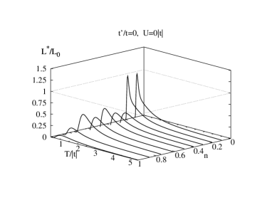
(b)

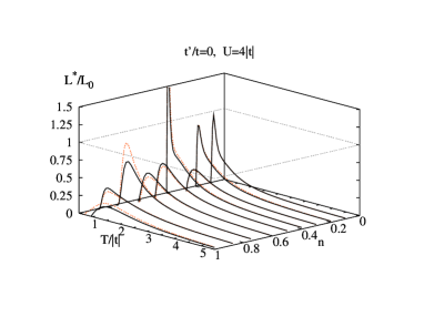
(c)

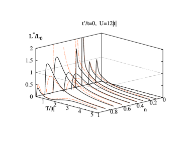
Figure 9: (color online) $L^{*}(T)/L_{0}$ as a function of filing $n$ and temperature $T$ (black line). The orange dotted line is the DC limit $L(0,T)$ for comparison. Note that for $U=0$ (a) there is no frequency dependence of $L(\omega,T)$ and $L^{*}(T)=L(0,T)$. The full $L(\omega,T)$ (not shown) compares similarly to the frequency dependence of the thermopower for $U=4|t|$ and $12|t|$ in Fig. 4.

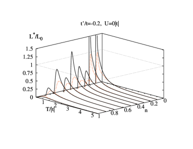
(a)	(b)
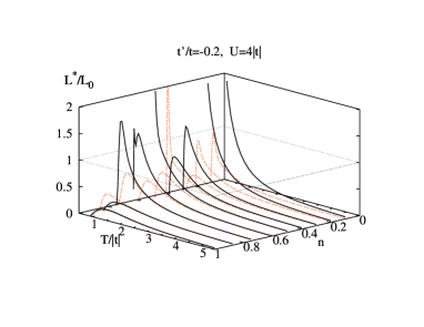
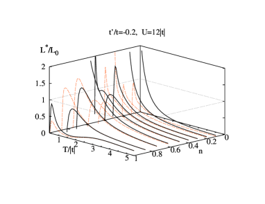
(c)	(d)

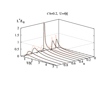
Figure 10: (color online) $L^{*}(T)/L_{0}$ as a function of filling $n$ and temperature $T$ for (a) $U=0$, (b) $U=4|t|$, and (c) $U=12|t|$. The full $L(\omega,T)$ compares similarly to frequency dependence of the thermopower. The orange dotted curve is the $t^{\prime}=0$ case to facilitate an easy comparison. (d) is an example of the other sign of $t^{\prime}$, namely, $t^{\prime}/t=0.2$.

Even though we do not explicitly calculate $S(\omega,T)$ for the $t$-$V$ model when $t^{\prime}\neq 0$, we comment that the introduction of $t^{\prime}$ causes the energy current operator not to commute with Hamiltonian. Consequently $S(\omega,T)$ is now no longer independent of $\omega$ and approaches $S^{*}(T)$ as $\omega\rightarrow\infty$ like in the Hubbard model. Presumably, the full frequency dependence is similar to that seen in the Hubbard model but has not been calculated explicitly.

Although not shown for the $t$-$V$ model, we point out that similar to the Hubbard model, the thermopower enhancement peak arises from the transport term of the thermopower almost exclusively as discussed in Sec. IV.1.2 and shown in Fig. 6.

V Lorenz number

The Lorenz number (Eq. 4) is an important quantity as it measures the ratio of the thermal to electrical conductivity. Further, it is a key ingredient to the FOM (containing both the thermopower and Lorenz number) which measures the efficiency of a thermoelectric material. Note that there is usually a contribution to the Lorenz number coming from lattice vibrations (phonons). In this work, however, we only consider the electronic contributions to the Lorenz number.

As noted in Ref. Peterson et al., 2007 the chemical potential is absent from Eq. 4 and the Lorenz number can be understood completely within the canonical ensemble. Evidently, it is determined through electron transport alone. At zero temperature it is well known that the Lorenz number is equal to the constant $L_{0}=(\pi k_{B}/\sqrt{3}q_{e})^{2}$ which is just the Wiedemann-Franz lawAshcroft and Mermin (1976); Ziman (1979).

As discussed in Ref. Peterson et al., 2007, for non-interacting systems, the limit $\lim_{T\rightarrow 0}L(\omega,T)=L_{0}$ comes from two effects. Similar to the thermopower, we attempt to limit the finite sized system induced divergences of the Lorenz number by forcing the subtle balances necessary to ensure a finite Lorenz number as $T\rightarrow 0$. The exact method used here is the same as in Ref. Peterson et al., 2007 and not repeated. Ultimately, we are able to control the divergences to a large degree, however, we are unable to answer the very interesting question of whether the value of $L_{0}$ is a universal constant independent of electron interactions.

Below we present $L^{*}(T)$ as a function of temperature and filling. The frequency dependence of $L(\omega,T)$ (not shown here) is comparable to $S(\omega,T)$ in that it is generally weak with a feature near $\omega=U$.

V.1 Hubbard with $t^{\prime}=0$

Fig. 9(a)-(c) shows the “normalized” high frequency Lorenz number $L^{*}(T)/L_{0}$ as a function of temperature and filling for the non-interacting, the weakly coupled, and the strongly coupled situations for the case of $t^{\prime}=0$. In Fig. 9(b)-(c) the DC limit of the full frequency dependent Lorenz number is also plotted, i.e., $L(0,T)/L_{0}$.

For the non-interacting case (Fig. 9(a)) $L^{*}(T)$ is suppressed at low temperatures as the filling increases towards half filling. For a thermodynamically large system the Lorenz number starts at $L_{0}$ and quickly decreases as a function of temperature similar to what is shown here. In the weakly coupled regime (Fig. 9(b)) $L^{*}(T)$ is very similar to the non-interacting case for fillings below approximately $n=0.4$. For $n\geq 0.5$, however, it is enhanced at low temperatures. The DC limit is quite similar to the infinite frequency limit showing the usefulness and accuracy of $L^{*}(T)$ in the weakly coupled regime. When the interactions are strong (Fig. 9(c)) there is a much stronger enhancement of $L^{*}(T)$ for $n\geq 0.3$ and the enhancement persists to higher temperatures. The DC limit in this case is not as similar to $L^{*}(T)$ as it is for the weakly coupled regime.

V.2 Hubbard with $t^{\prime}\neq 0$

For non-zero $t^{\prime}$ we plot $L^{*}(T)/L_{0}$ as a function of filling and temperature along with $L^{*}(T)/L_{0}$ for the $t^{\prime}=0$ to ease comparison in Fig. 10(a)-(d).

For the same sign of $t^{\prime}<0$ that produced the thermopower enhancement the Lorenz number in Fig. 10(a)-(c) is also enhanced compared to the $t^{\prime}=0$ situation at low temperatures. This enhancement is also more pronounced for low than for high fillings and increases with increasing interaction strength $U$, especially close to half filling.

When $t^{\prime}>0$ in the weakly coupled regime (Fig. 10(d)) the Lorenz number is very slightly suppressed compared to the $t^{\prime}=0$ situation as one would expect from the $t^{\prime}<0$ results and the previous investigation of the thermopower.

Generally, for both $t^{\prime}=0$ and $t^{\prime}\neq 0$ the Lorenz number is appreciably below $L_{0}$ for all temperatures above approximately $T\sim 1.5|t|$.

VI Figure of merit

(a)

(b)

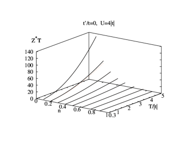
(c)

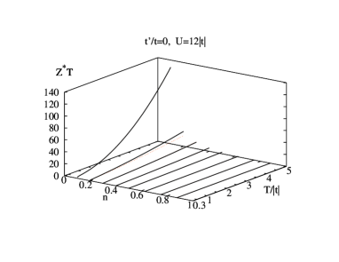
Figure 11: (color online) $Z^{*}(T)T$ as a function of filling $n$ and temperature $T$ as the solid black line for $U=0$ (a), $U=4|t|$ (b), and $U=12|t|$ (c). The orange dotted curve is the DC limit of the full $Z(\omega,T)T$ for comparison, i.e., $Z(0,T)T$. Note that for $U=0$ (a) there is no frequency dependence.

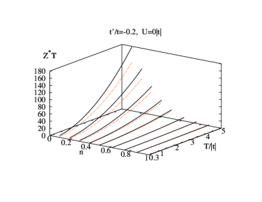
(a)	(b)
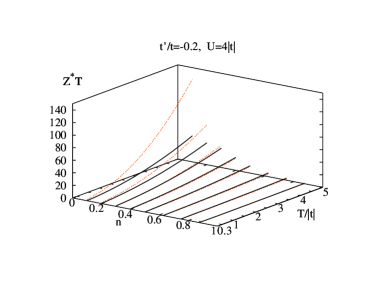
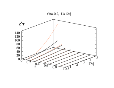
(c)	(d)

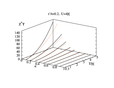
Figure 12: (color online) $Z^{*}(T)T$ as a function of filling $n$ and temperature $T$ for (a) $U=0$, (b) $U=4|t|$, and (c) $U=12|t|$. The full frequency dependent $Z(\omega,T)T$ compares similarly to the frequency dependence of the thermopower. The orange dotted curve is for $t^{\prime}=0$ to facilitate an easy comparison. For an example of the other sign of $t^{\prime}$ we plot the situation $t^{\prime}/t=0.2$ in (d).

The figure of merit is the number that is most important when it comes to technological applications regarding thermoelectrics, as mentioned above, being a measure of thermoelectrical efficiency. In our calculations we are ignoring the lattice contribution to the Lorenz number so our FOM calculated is that due to only electronic contributions.

Using the “tricks” to handle finite size effects for $S^{*}(T)$ and $L^{*}(T)$, c.f. Ref. Peterson et al., 2007, we calculate the high frequency expansion of the FOM ($Z^{*}(T)T$) given in Eq. 8.

A large FOM can arise in essentially two ways. One way is for the thermopower, which is squared in the numerator, to be large. The other is for the Lorenz number in the denominator to be small. The Lorenz number has been shown in Sec V to tend to zero as the temperature tends to infinity. The thermopower, on the other hand, reaches a constant, and finite, MH limit as $T\rightarrow\infty$. Hence, the electronic contribution to the FOM will eventually grow to infinity as the temperature is increased without bound.

In the following subsections we plot $Z(\omega,T)T$ as a function of $T$ and filling $n$.

VI.1 Hubbard with $t^{\prime}=0$

Fig. 11(a)-(c) shows the FOM for the $t^{\prime}=0$ Hubbard model for the non-interacting case, the weakly coupled case, and the strongly coupled case. Also plotted is the DC limit of the full frequency dependent FOM. In the non-interacting case (Fig. 11(a)) the FOM grows apparently quadratically in temperature with a coefficient that decreases inversely with filling. This behavior is seen in the weakly coupled and strongly coupled cases as well, c.f. Fig. 11(b)-(c), although the FOM is decreased more for lower fillings.

The full frequency behavior of the FOM (not shown) is very similar to the high frequency limit, evidently because the differences in the two limits for the thermopower and Lorenz number largely cancel one another out.

VI.2 Hubbard with $t^{\prime}\neq 0$

In Fig. 12(a)-(c) and Fig. 12(d) we investigate the effects of frustration on the FOM for the $t^{\prime}<0$ and $t^{\prime}>0$ cases, respectively.

For the situation that produced a low temperature enhancement in the thermopower and Lorenz number ($t^{\prime}<0$) the FOM is suppressed compared to $t^{\prime}=0$ except for the non-interacting case where they are very similar. The larger interaction strength has the effect of further suppressing the FOM especially for low fillings.

Alternatively, the case of $t^{\prime}>0$ that produced suppression in both $S^{*}(T)$ and $L^{*}(T)$ has a very slight enhancement in the FOM shown in Fig. 12(d). This nicely illustrates the complicated way in which the thermopower and Lorenz number combine to produce the FOM.

VII Conclusion

We have computed thermoelectrical properties of the Hubbard model and the spin-less fermion $t$-$V$ model on one-dimensional rings investigating, in particular, the thermopower (Hubbard and $t$-$V$), Lorenz number, and figure of merit (Hubbard only). Our calculations are the first detailed calculations of these thermoelectric variables in the literature for strongly correlated models. By adding a second neighbor hopping term with amplitude $t^{\prime}$, both positive and negative, we were able to destroy the integrability of these models and induce frustration. For $t^{\prime}<0$ the Hubbard and $t$-$V$ model displayed an enhanced thermopower at low to intermediate temperatures. For the Hubbard model the Lorenz number was also found to have low temperature enhancements for $t^{\prime}<0$. However, the FOM did not produce the same enhancement for $t^{\prime}<0$ but instead a suppression for non-zero interaction strength $U$. Although, the FOM was modestly enhanced by the opposite hopping $t^{\prime}>0$ at low fillings.

For the Hubbard model, the thermopower had a generally weak frequency dependence other than a sometimes large feature near $\omega\sim U$. This behavior was also obtained, but not shown here, for the Lorenz number and FOM. This has the consequence that the high frequency versions of the thermopower, Lorenz number, and FOM recently proposed by ShastryShastry (2006a, b, 2007) provide a good approximation to the full dynamical quantities for most values of the system parameters.