Co-orbital Oligarchy

Abstract

We present a systematic examination of the changes in semi-major axis caused by the mutual interactions of a group of massive bodies orbiting a central star in the presence of eccentricity dissipation. For parameters relevant to the oligarchic stage of planet formation, dynamical friction keeps the typical eccentricities small and prevents orbit crossing. Interactions at impact parameters greater than several Hill radii cause the protoplanets to repel each other; if the impact parameter is instead much less than the Hill radius, the protoplanets shift slightly in semi-major axis but remain otherwise unperturbed. If the orbits of two or more protoplanets are separated by less than a Hill radius, they are each pushed towards an equilibrium spacing between their neighbors and can exist as a stable co-orbital system. In the shear-dominated oligarchic phase of planet formation we show that the feeding zones contain several oligarchs instead of only one. Growth of the protoplanets in the oligarchic phase drives the disk to an equilibrium configuration that depends on the mass ratio of protoplanets to planetesimals, $\Sigma/\sigma$. Early in the oligarchic phase, when $\Sigma/\sigma$ is low, the spacing between rows of co-orbital oligarchs are about 5 Hill radii wide, rather than the $10$ Hill radii cited in the literature. It is likely that at the end of oligarchy the average number of co-orbital oligarchs is greater than unity. In the outer solar system this raises the disk mass required to form the ice giants. In the inner solar system this lowers the mass of the final oligarchs and requires more giant impacts than previously estimated. This result provides additional evidence that Mars is not an untouched leftover from the oligarchic phase, but must be composed of several oligarchs assembled through giant impacts.

1. Introduction

The early stages in the formation of planetary systems are well described by statistical calculations of the evolution of mass distributions and velocity dispersions. As larger bodies accumulate from the swarm of proto-planetary material, their individual dynamics begin to dominate their evolution. Lissauer (1987) pointed out that the finite cross-section for accretion limits the growth of each protoplanet. This is now known as the “oligarchic phase.” (Kokubo & Ida, 1998). Numerical (Kenyon & Bromley, 2006; Ford & Chiang, 2007; Levison & Morbidelli, 2007) and analytical (Goldreich et al., 2004a) work has explored the transition from oligarchic growth to the chaotic final assembly of the planets. In this work we examine the interactions of a moderate number of protoplanets in an oligarchic configuration and find that neighboring protoplanets stabilize co-orbital systems of two or more protoplanets. We present a new picture of oligarchy in which each part of the disk is not ruled by one but by several protoplanets having almost the same semi-major axis.

Our approach is to systematize the interactions between each pair of protoplanets in a disk where a swarm of small icy or rocky bodies, the planetesimals, contain most of the mass. The planetesimals provide dynamical friction that circularizes the orbits of the protoplanets. The total mass in planetesimals at this stage is more than that in protoplanets so dynamical friction balances the excitations of protoplanets’ eccentricities. We characterize the orbital evolution of a protoplanet as a sequence of interactions occurring each time it experiences a conjunction with another protoplanet. The number density of protoplanets is low enough that it is safe to neglect interactions between three or more protoplanets.

To confirm our description of the dynamics and explore its application to more realistic proto-planetary situations we perform many numerical N-body integrations. We use an algorithm optimized for mostly circular orbits around a massive central body. As integration variables we choose six constants of the motion of an unperturbed Keplerian orbit. As the interactions between the other bodies in the simulations are typically weak compared to the central force, the variables evolve slowly. We employ a 4th-order Runge-Kutta integration algorithm with adaptive time-steps (Press et al., 1992) to integrate the differential equations. During periods of little interaction, the slow evolution of our variables permits large time-steps.

During a close encounter, the inter-particle gravitational attraction becomes comparable to the force from the central star. In the limit that the mutual force between a pair of particles is much stronger than the central force, the motion can be more efficiently described as a perturbation of the two-body orbital solution of the bodies around each other. We choose two new sets of variables: one to describe the orbit of the center-of-mass of the pair around the central star, and another for relative motion of the two interacting objects. These variables are evolved under the influence of the remaining particles and the central force from the star.

Dynamical friction, when present in the simulations, is included with an analytic term that damps the eccentricities and inclinations of each body with a specified timescale. All of the simulations described in this work were performed on Caltech’s Division of Geological and Planetary Sciences Dell cluster.

We review of some basic results from the three-body problem in section 2, and describe the modifications of these results due to eccentricity dissipation. In section 3, we generalize the results of the three-body case to an arbitrary number of bodies, and show the resulting formation and stability of co-orbital sub-systems. Section 4 demonstrates that an oligarchic configuration with no initial co-orbital systems can acquire such systems as the oligarchs grow. Section 5 describes our investigation into the properties of a co-orbital oligarchy, and section 6 places these results in the context of the final stages of planet formation. The conclusions are summarized in section 7.

2. The Three-Body Problem

The circular restricted planar three-body problem refers to a system of a zero mass test particle and two massive particles on a circular orbit. We call the most massive object the star and the other the protoplanet. The mass ratio of the protoplanet to the star is $\mu$. Their orbit has a semi-major axis $a$ and an orbital frequency $\Omega$. The test particle follows an initially circular orbit with semi-major axis $a_{\rm tp}=a(1+x)$ with $x\ll 1$. Since the semi-major axes of the protoplanet and the test particle are close, they rarely approach each other. For small $x$, the angular separation between the two bodies changes at the rate $(3/2)\Omega x$ per unit time. Changes in the eccentricity and semi-major axis of the test particle occur only when it reaches conjunction with the protoplanet.

The natural scale for $xa$ is the Hill radius of the protoplanet, $R_{H}\equiv(\mu/3)^{1/3}a$. For interactions at impact parameters larger than about four Hill radii, the effects of the protoplanet can be treated as a perturbation to the Keplerian orbit of the test particle. These changes can be calculated analytically. To first order in $\mu$, the change in eccentricity is $e_{k}=A_{k}\mu x^{-2}$, where $A_{k}=(8/9)[2K_{0}(2/3)+K_{1}(2/3)]\approx 2.24$ and $K_{0}$ and $K_{1}$ are modified Bessel functions of the second kind (Goldreich & Tremaine, 1978; Petit & Henon, 1986).

The change in semi-major axis of the test particle can be calculated from an integral of the motion, the Jacobi constant: $C_{\rm J}\equiv E-\Omega H$, where $E$ and $H$ and are energy and angular momentum per unit mass of the test particle. Rewriting $C_{\rm J}$ in terms of $x$ and $e$, we find that

$$\frac{3}{4}x^{2}-e^{2}=~{}{\rm const}.$$ (1)

If the encounter increases $e$, $|x|$ must also increase. The change in $x$ resulting from a single interaction on an initially circular orbit is

$$\Delta x=(2/3)e_{k}^{2}/x=(2/3)A_{k}^{2}\mu^{2}x^{-5}.$$ (2)

The contributions of later conjunctions add to the eccentricity as vectors and do not increase the magnitude of the eccentricity by $e_{k}$. Because of this the semi-major axis of the test particle generally does not evolve further than the initial change $\Delta x$. Two alternatives are if the test particle is in resonance with the protoplanet, or if its orbit is chaotic. If the test particle is in resonance, the eccentricity of the particle varies as it librates. Chaotic orbits occur when each excitation is strong enough to change the angle of the next conjunction substantially; in this case $e$ and $x$ evolve stochastically (Wisdom, 1980; Duncan et al., 1989).

Orbits with $x$ between 2-4 $R_{H}/a$ can penetrate the Hill sphere and experience large changes in $e$ and $a$. This regime is highly sensitive to initial conditions, so we only offer a qualitative description. Particles on these orbits tend to receive eccentricities of the order the Hill eccentricity, $e_{H}\equiv R_{H}/a$, and accordingly change their semi-major axes by $\sim R_{H}$. We will call this the “strong-scattering regime” of separations. A fraction of these trajectories collide with the protoplanet; these orbits are responsible for proto-planetary accretion (Greenzweig & Lissauer, 1990; Dones & Tremaine, 1993).

For $x\lesssim R_{H}/a$, the small torque from the protoplanet is sufficient to cause the particle to pass through $x=0$. The particle then returns to its original separation on the other side of the protoplanet’s orbit. These are the famous horseshoe orbits that are related to the 1:1 mean-motion resonance. The change in eccentricity from an initially circular orbit that experiences this interaction can be calculated analytically (Petit & Henon, 1986): $e_{k}=2^{2/3}3^{-3/2}5\Gamma(2/3)\mu^{1/3}{\rm exp}(-(8\pi/9)\mu x^{-3})$, where $\Gamma(2/3)$ is the usual Gamma function. Since this interaction is very slow compared to the orbital period, the eccentricity change is exponentially small as the separation goes to zero. As in the case of the distant encounters, the conservation of the Jacobi constant requires that $x$ increases as the eccentricity increases (equation 1). Then,

$$\Delta x=2.83\frac{\mu^{2/3}}{x}{\rm exp}(-5.58\mu x^{-3}).$$ (3)

To apply these results to proto-planetary disks, we must allow the test particle to have mass. We now refer to both of the bodies as protoplanets, each having mass ratios with the central object of $\mu_{1}$ and $\mu_{2}$. The change in their total separation after one conjunction is given by equations 2 and 3 with $\mu=\mu_{1}+\mu_{2}$.

Figure 1.— The change in semi-major axis after a conjunction of two bodies on initially circular orbits whose masses are smaller than that of the star by the ratio $\mu=3\times 10^{-9}$, plotted as a function of the initial separation. The points are calculated with numerical integrations, while the dashed lines show the analytic results, equations 2 and 3. At the smallest impact parameters the bodies switch orbits; in this case we have measured the change relative to the initial semi-major axis of the other protoplanet. The horizontal lines separate the regions of $x$ that are referred to in the text.

Figure 1 plots the change in $a$ after one conjunction of two equal mass protoplanets as measured from numerical integrations. All three types of interactions described above are visible in the appropriate regime of $x$. Each point corresponds to a single integration of two bodies on initially circular orbits separated by $x$. For the horseshoe-type interactions, each protoplanet moves a distance almost equal to $x$; we only plot the change in separation: $\Delta a_{\rm H.S.}=|\Delta a|-|x|a$. The regimes of the three types of interactions are marked in the figure. The dashed line in the low $x$ regime plots the analytic expression calculated from equation 3. The separations that are the most strongly scattered lie between $2-4R_{H}$, surrounding the impact parameters for which collisions occur. For larger separations the numerical calculation approaches the limiting expression of equation 2, which is plotted as another dashed line.

The sea of planetesimals modifies the dynamics of the protoplanets. If the planetesimals have radii less than $\sim 1~{}{\rm km}$, their own collisions balance the excitations caused by the protoplanets. At the same time, the planetesimals provide dynamical friction that damps the eccentricities of the protoplanets. When the typical eccentricities of the protoplanets and the planetesimals are lower than the Hill eccentricity of the protoplanets, this configuration is said to be shear-dominated: the relative velocity between objects is set by the difference in orbital frequency of nearby orbits. In the shear-dominated eccentricity regime, the rate of dynamical friction is (Goldreich et al., 2004b):

$$-\frac{1}{e}\frac{de}{dt}=C_{d}\frac{\sigma\Omega}{\rho R}\alpha^{-2}=\frac{1}{\tau_{\rm d}},$$ (4)

where $R$ and $\rho$ are the radius and density of a protoplanet, $\sigma$ is the surface mass density in planetesimals, $\alpha$ is the ratio $R/R_{H}$, and $C_{d}$ is a dimensionless coefficient of order unity. Recent studies have found values for $C_{d}$ between 1.2 and 6.2 (Ohtsuki et. al. 2002; Schlichting and Sari, in preparation). For this work, we use a value of 1.2. For parameters characteristic of the last stages of planet formation, $\tau_{d}\gg 2\pi/\Omega$. The interactions of the protoplanets during an encounter are unaffected by dynamical friction and produce the change in $e$ and $a$ as described above. In between protoplanet conjunctions, the dynamical friction circularizes the orbits of the protoplanets. The next encounter that increases $e$ further increases $x$ to conserve the Jacobi constant. The balance between excitations and dynamical friction keeps the eccentricities of the protoplanets bounded and small, but their separation increases after each encounter. This mechanism for orbital repulsion has been previously identified by Kokubo & Ida (1995), who provide a timescale for this process. We alternatively derive the timescale by treating the repulsion as a type of migration in semi-major axis. The magnitude of the rate depends on the strength of the damping; it is maximal if all the eccentricity is damped before the next encounter, or $\tau_{d}\ll 4\pi/(3\Omega x)$. In this case, a protoplanet with a mass ratio $\mu_{1}$ and semi-major axis $a_{1}$ interacting with a protoplanet with a mass ratio $\mu_{2}$ in the regime of distant encounters is repelled at the rate:

$$\frac{1}{a_{1}}\frac{da_{1}}{dt}=\frac{A_{k}^{2}}{2\pi}\mu_{2}(\mu_{1}+\mu_{2})x^{-4}\Omega.$$ (5)

For protoplanets in the horseshoe regime, the repulsion of each interaction is given by equation 3. These encounters increase the separation at an exponentially slower rate of:

$$\frac{1}{a_{1}}\frac{da_{1}}{dt}=0.67\mu_{2}(\mu_{1}+\mu_{2})^{-2/3}{\rm exp}(-5.58(\mu_{1}+\mu_{2})x^{-3})\Omega.$$ (6)

If instead $\tau_{d}\gg 4\pi/(3\Omega x)$, the eccentricity of the protoplanet is not completely damped away before the next conjunction restores the protoplanet to $e\sim e_{k}$. The rate at which the separation increases is then related to the rate of dynamical friction, $\dot{a}\propto e_{k}\dot{e}/x$. Qualitatively, this rate is slower than those of equations 5 and 6 by $(\tau_{d}\Omega x)^{-1}$. We focus on the maximally damped case where $\tau_{d}\ll 4\pi/(3\Omega x)$.

3. The Damped N-body Problem

Having characterized the interactions between pairs of protoplanets, we next examine a disk of protoplanets with surface mass density $\Sigma$. Each pair of protoplanets interacts according to their separations as described in section 2. If the typical spacing is of order $R_{H}$, the closest encounters between protoplanets causes changes in semi-major axes of about $R_{H}$ and eccentricity excitations to $e_{H}$. The strong scatterings may also cause the two protoplanets to collide. If the planetesimals are shear-dominated and their mass is greater than the mass in protoplanets, the eccentricities of the protoplanets are held significantly below $e_{H}$ by dynamical friction (Goldreich et al., 2004b), and the distribution of their eccentricities can be calculated analytically (Collins & Sari, 2006; Collins et al., 2006). If the scatterings and collisions rearrange the disk such that there are no protoplanets with separations of about $2-4R_{H}$, the evolution is subsequently given by only the gentle pushing of distant interactions (Kokubo & Ida, 1995). However, there is another channel besides collisions through which the protoplanets may achieve stability: achieving a semi-major axis very near that of another protoplanet.

A large spacing between two protoplanets ensures they will not strongly-scatter each other. However, a very small difference in semi-major axis can also provide this safety (see figure 1 and equation 6). Protoplanets separated by less than $2R_{H}$ provide torques on each other during an encounter that switch the order of their semi-major axis and reverse their relative angular motion before they can get very close. Their mutual interactions are also very rare, since their relative orbital frequency is proportional to their separation. Protoplanets close to co-rotation are almost invisible to each other, however these protoplanets experience the same $\dot{a}/a$ from the farther protoplanets as given by equation 5. We call the group of the protoplanets with almost the same semi-major axis a “co-orbital group” and use the label $N$ to refer to the number of protoplanets it contains. The protoplanets within a single group can have any mass, although for simplicity in the following discussion we assume equal masses of each.

Different co-orbital groups repel each other at the rate of equation 5. For equally spaced rows of the same number of equal mass protoplanets, the migration caused by interior groups in the disk exactly cancels the migration caused by the exterior groups. We say that the protoplanets in this configuration are separated by their “equilibrium spacing.” We define a quantity, $y$, to designate the distance between a single protoplanet and the position where it would be in equilibrium with the interior and exterior groups. The near cancellation of the exterior and interior repulsions decreases $y$, pushing displaced protoplanets towards their equilibrium spacing. The migration rate of a single protoplanet near the equilibrium spacing of its group be calculated by expanding equation 5 to first order in $y$ and taking the difference between interior and exterior contributions:

$$\frac{1}{y}\frac{dy}{dt}\approx\frac{a}{y}\sum_{i=1}^{\infty}8N\frac{\dot{a}}{a}\frac{y}{ix~{}a}\approx 131N\left(\frac{x~{}a}{R_{H}}\right)^{-5}e_{H}\Omega,$$ (7)

where we assume that the other co-orbital groups in the disk are regularly spaced by $\Delta a=x~{}a$ and contain $N$ protoplanets of a single mass ratio. Each term in the summation represents a pair of neighboring groups for which $\dot{a}$ is evaluated at the unitless separation $ix$. Since the repulsion rate is a sharp function of the separation, the nearest neighbors dominate. The coefficient in equation 7 takes a value of 121 when only the closest neighbors are included ($i=1$ only). Including an infinite number of neighbors increases the coefficent by a factor of $1+2^{-5}+3^{-5}+...$, only about 8 percent.

The dynamics above describe an oligarchic proto-planetary disk as a collection of co-orbital groups each separated by several Hill radii. It is necessary though to constrain such parameters as the typical spacing between stable orbits and the relative population of co-orbital systems. To determine these quantities we perform full numerical integrations. Given a set of initial conditions in the strong-scattering regime, what is the configuration of the protoplanets when they reach a stable state?

We have simulated an annulus containing twenty protoplanets, each with a mass ratio of $\mu=1.5\times 10^{-9}$ to the central star. The protoplanets start on circular orbits spaced uniformly in semi-major axis. We dissipate the eccentricities of the protoplanets on a timescale of 80 orbits; for parameters in the terrestrial region of the Solar System and using $C_{d}=1.2$, this corresponds to a planetesimal mass surface density of about 8 ${\rm g~{}cm^{-2}}$. We allow the protoplanets to collide with each other setting $\alpha^{-1}=227$; this corresponds to a density of $5~{}{\rm g~{}cm^{-3}}$.

We examine two initial compact separations: 1.0 $R_{H}$ (set A) and 2.5 $R_{H}$ (set B). For each initial separation we run 1000 simulations starting from different randomly chosen initial phases. After $6\times 10^{3}$ orbital periods the orbits of the protoplanets have stabilized and we stop the simulations. To determine the configuration of the protoplanets, we write an ordered list of the semi-major axis of the protoplanets in each simulation. We then measure the separation between each adjacent pair of protoplanets (defined as a positive quantity). If the semi-major axes of two or more protoplanets are within 2 $R_{H}$, we assume they are part of the same co-orbital group. The average semi-major axis is calculated for each group. The distance of each member of a group from the average semi-major axis we call the “intra-group separation.” These values can be either positive or negative and, for the co-orbital scenarios we are expecting, are typically smaller than $1R_{H}$.

When one protoplanet is more than 2 $R_{H}$ from the next protoplanet, we assume that the next protoplanet is either alone or belongs to the next co-orbital group. The spacing between the average semi-major axis of one group and the semi-major axis of the next protoplanet or co-orbital group we call the “inter-group spacing.” These separations are by definition positive.

Finally we create a histogram of both the intra-group separations and the inter-group separations of all the simulations in the set. For reference, the initial configuration of the simulations of set B contains no co-orbital groups. The resulting histogram would depict no intra-group separations, and have only one non-zero bin representing the inter-group separations of $x=2.5R_{H}$.

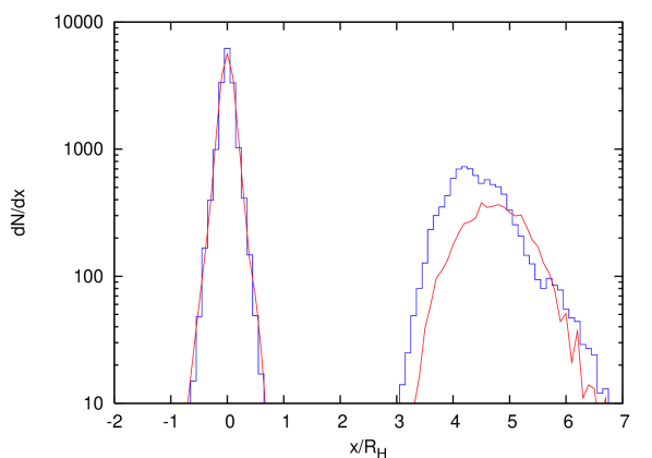
Figure 2.— Histogram of the intra-group and inter-group separations between protoplanets in two sets of numerical simulations. Each simulation integrates 20 protoplanets with mass ratios of $3\times 10^{-9}$ compared to the central mass. They begin on circular orbits with uniform separations in semi-major axis; each set of simulations consists of 1000 integrations with random initial phases. The eccentricities of the protoplanets are damped with a timescale of 80 orbits. The smooth line (red) represents the simulations of set A, with an initial spacing of 1.0 $R_{H}$, and the stepped line (blue) shows simulations of set B, which have an initial spacing of 2.5 $R_{H}$.

Figure 2 shows the histograms of the final spacings of the two sets of simulations. The spacings in set A are shown in the smooth line (red), and those of set B are shown in the stepped line (blue). The initial closely-spaced configurations did not survive. The distributions plotted in figure 2 reveal that none of the spacings between neighboring protoplanets are in the strong scattering regime, since it is unstable. This validates the arbitrary choice of 2 $R_{H}$ as the boundary in the construction of figure 2; any choice between 1 and 3 $R_{H}$ would not affect the results.

The size of the peak of intra-group spacings shows that most of the protoplanets in the disk are co-orbital with at least one other body. The shape shows that the spread of semi-major axis of each co-orbital group is small. This is consistent with equation 7, since endpoint of these simulations is late enough to allow significant co-orbital shrinking. The second peak in figure 2 represents the inter-group separation. The median inter-group separation in the two sets are $4.8R_{H}$ and $4.4R_{H}$. This is much less than the $10R_{H}$ usually assumed for the spacing between protoplanets in oligarchic planet formation (Kokubo & Ida, 1998, 2002; Thommes et al., 2003; Weidenschilling, 2005).

Figure 2 motivates a description of the final configuration of each simulation as containing a certain number of co-orbital groups that are separated from each other by $4-5R_{H}$. Each of these co-orbital groups is further described by its occupancy number $N$. For the simulations of set A, the average occupancy $\langle N\rangle=2.8$, and for set B, $\langle N\rangle=1.8$. Since the simulated annulus is small, the co-orbital groups that form near the edge are underpopulated compared to the rest of the disk. For the half of the co-orbital groups with semi-major axes closest to the center of the annulus, $\langle N\rangle$ is higher: $\langle N\rangle=3.5$ for set A and $\langle N\rangle=2.0$ for set B.

4. Oligarchic Planet Formation

The simulations of section 3 demonstrate the transition from a disordered swarm of protoplanets to an orderly configuration of co-orbital rows each containing several protoplanets. The slow accretion of planetesimals onto the protoplanets causes an initially stable configuration to become unstable. The protoplanets stabilize by reaching a new configuration with a different average number of co-orbital bodies. To demonstrate this process we simulate a disk of protoplanets and allow accretion of the planetesimals.

We use initial conditions similar to the current picture of a disk with no co-orbital protoplanets, placing twenty protoplanets with mass ratios $\mu=3\times 10^{-9}$ on circular orbits spaced by $5R_{H}$. This spacing is the maximum impact parameter at which a protoplanet can accrete a planetesimal (Greenberg et al., 1991) and a typical stable spacing between oligarchic zones (figure 2). For the terrestrial region around a solar-mass star, this mass ratio corresponds to protoplanets of mass $6\times 10^{24}~{}{\rm g}$, far below the final expected protoplanet mass (see section 6). Our initial configuration has no co-orbital systems. We include a mass growth term in the integration to represent the accretion of planetesimals onto the protoplanets in the regime where the eccentricity of the planetesimals $e_{p}$ obeys $\alpha^{1/2}e_{H}<e_{p}<e_{H}$ (Dones & Tremaine, 1993):

$$\frac{1}{M}\frac{dM}{dt}=2.4\frac{\sigma\Omega}{\rho R}\frac{1}{\alpha}\frac{e_{H}}{e_{p}}.$$ (8)

Protoplanet-protoplanet collisions are allowed. For simplicity we assume the planetesimal disk does not evolve in response to the protoplanets. Eccentricity damping of the protoplanets from dynamical friction of the planetesimals is included. The damping timescale, 80 orbits, and growth timescale, 4800 orbits, correspond to a planetesimal surface density of $10~{}{\rm g~{}cm^{-2}}$ and a typical planetesimal eccentricity of $e_{p}=5\times 10^{-4}$. We have again used the value $C_{d}=1.2$. These parameters imply a planetesimal radius of $\sim 100$ m, assuming that the planetesimal stirring by the protoplanets is balanced by physical collisions. Each protoplanet has a density of $5~{}{\rm g~{}cm^{-3}}$. The annulus of bodies is centered at 1 AU. We simulate 1000 systems, each beginning with different randomly chosen orbital phases. Figure 3 shows the evolution of the semi-major axis of the protoplanets in one of the simulations as a function of time; other simulations behave similarly.

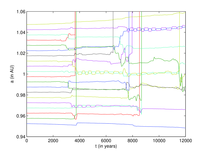
Figure 3.— Semi-major axes of the protoplanets vs time in a simulation of oligarchic growth around a solar mass star. The initial mass of each protoplanet is $6\times 10^{24}~{}{\rm g}$ and each is spaced 5 $R_{H}$ from its nearest neighbor. The planetesimals have a surface density of $10~{}{\rm g~{}cm^{-2}}$ and an eccentricity $e_{p}=5\times 10^{-4}$. These parameters correspond to a damping timescale of 80 years and a growth timescale of 4800 years. The sharp vertical lines indicate a collision between two bodies; the resulting protoplanet has the sum of the masses and a velocity chosen to conserve the linear momentum of the parent bodies.

If there were no accretion, the protoplanets would preserve their original spacing indefinitely, aside from a slow spreading at the edges of the annulus. However, the spacing in units of Hill radii decreases as the protoplanets grow. Eventually their interactions become strong enough to cause collisions and large scatterings. This epoch of reconfiguration occurs after a time of approximately $4000$ orbits in the simulation plotted in figure 3. At this point the mass of protoplanets has increased by roughly a factor of 2.3, meaning the spacing in units of Hill radii has decreased by a factor of 1.3. We would expect the chaotic reconfiguration to restore the typical spacing to about $5R_{H}$ by reducing the number of oligarchic zones. The figure, in fact, shows 13 zones after the first reconfiguration, compared to 20 before. Three protoplanets have collided, and four have formed co-orbital groups of $N=2$. The co-orbital pairs are visibly tightened over the timescale predicted by equation 7, which for the parameters of this simulation is about $\Delta t\approx 3\times 10^{3}$ years. The configuration is then stable until the growth of the bodies again lowers their separation into the strong-scattering regime at a time of $1.1\times 10^{4}$ years.

The other realizations of this simulation show similar results. We find an average co-orbital population of $\langle N\rangle=1.2$ in the middle of the annulus after the first reconfiguration. This value is lower than those found in section 3 because the protoplanets begin to strongly-scatter each other when they are just closer than the stable spacing. Only a few protoplanets can collide or join a co-orbital group before the disk becomes stable again. As described in the paradigm of Kokubo & Ida (1995), a realistic proto-planetary disk in the oligarchic phases experiences many such epochs of instability as the oligarchs grow to their final sizes.

5. The Equilibrium Co-orbital Number

As the protoplanets evolve, they experience many epochs of reconfiguration that change the typical co-orbital number. The examples given in previous sections of this work show the result of a single reconfiguration. Our choices of initial conditions with the initial co-orbital number $\langle N\rangle_{i}=1$ have resulted in a higher final co-orbital number $\langle N\rangle_{f}$. If instead, $\langle N\rangle_{i}$ is very high, the final co-orbital number must decrease. As the disk evolves, $\langle N\rangle$ is driven to an equilibrium value where each reconfiguration leaves $\langle N\rangle$ unchanged. This value, $\langle N\rangle_{\rm eq}$, is the number that is physically relevant to the proto-planetary disk.

We use a series of simulations to determine $\langle N\rangle_{\rm eq}$ at a fixed value of $\Sigma$ and $\sigma$. Each individual simulation contains forty co-orbital groups separated by $4~{}R_{H}$. This spacing ensures each simulation experiences a chaotic reconfiguration. The number of oligarchs in each group is chosen randomly to achieve the desired $\langle N\rangle_{i}$. All oligarchs begin with $e=e_{H}$ and $i=i_{H}$ to avoid the maximal collision rate that occurs if $e<\alpha^{1/2}e_{H}$ (Goldreich et al., 2004b). The initial orbital phase, longitude of periapse, and line of nodes are chosen randomly. We set a lower limit to the allowed inclination to prevent it from being damped to unreasonably small values. The results of the simulations are insensitive to the value of this limit if it is smaller than $i_{H}$; we choose $10^{-3}~{}i_{H}$.

We include an additional force in the simulations to prevent the initial annulus from increasing in width. This extra force pushes the semi-major axis of a protoplanet back into the annulus at a specified timescale. We choose this timescale to be longer than the typical time between encounters, $(\Omega x)^{-1}$, so that multiple protoplanets are not pushed to the boundary of the annulus without having the chance to encounter a protoplanet a few Hill radii away. Collisions between protoplanets are allowed, but the protoplanets are not allowed to accrete the planetesimals. Each simulation is stopped when there has not been a close encounter for $1.6\times 10^{4}$ orbits. Inspection of the simulation results reveals that this stopping criteria is sufficient for the disk to have reached an oligarchic state. We measure the final semi-major axes of the protoplanets to determine $N$ for each co-orbital group. For each set of parameters ($\Sigma$, $\sigma$, and $\langle N\rangle_{i}$) we perform 100 simulations.

Figure 4.— The final $\langle N\rangle$ of simulations against the initial $\langle N\rangle$ for $\Sigma=0.9~{}{\rm g~{}cm^{-2}}$ and $\sigma=9.1~{}{\rm g~{}cm^{-2}}$. For each value of $\langle N\rangle_{i}$ the mass of each protoplanet is adjusted to keep $\Sigma$ constant. The dashed lines denote the average value plus and minus one standard deviation of the measurements. The solid line illustrates where $\langle N\rangle_{i}=\langle N\rangle_{f}$.

The numerical values we have chosen for these simulations reflect planet formation in the terrestrial region. We center the annulus of the simulations at 1 AU. We adopt the minimum mass solar nebula for total mass of solids in the annulus, $\Sigma+\sigma=10~{}{\rm g~{}cm^{-2}}$ (Hayashi, 1981), and keep this value fixed throughout all the simulations. Figure 4 plots the results of simulations for $\Sigma/\sigma=1/10$. The points connected by the solid line show the average $\langle N\rangle_{f}$ of each set of simulations, while the dashed lines show the average value plus and minus one standard deviation of those measurements. For reference, we plot another solid line corresponding to $\langle N\rangle_{i}=\langle N\rangle_{f}$. The points at low $\langle N\rangle_{i}$ show a similarity to the results of the simulations of sections 3 and 4: stability is reached by increasing the number of oligarchs in each co-orbital groups. Once $\langle N\rangle_{i}$ is too high, the chaotic reconfiguration results in an oligarchy with lower $\langle N\rangle$. Figure 4 depicts a feedback cycle that drives $\langle N\rangle$ towards an equilibrium value that remains unchanged by a reconfiguration. For $\Sigma/\sigma=1/10$, we find $\langle N\rangle_{\rm eq}\approx 2.5$. The intersection of the dotted lines with $\langle N\rangle_{i}=\langle N\rangle_{f}$ yields the one standard deviation range of $\langle N\rangle_{\rm eq}$, $2-3.2$.

Figure 5.— The final average mass ratio, $\langle\mu\rangle$, of the protoplanets plotted against the final $\langle N\rangle$ for ratio of surface densities of $\Sigma/\sigma=1/10$. Each symbol corresponds to a value of $\langle N\rangle_{i}$. The solid lines plot lines of constant $\Sigma$ for values of $\langle x\rangle$ one standard deviation away from the best fit curve of constant $\Sigma$ to the simulations with $\langle N\rangle_{i}=2.5$.

The cause of the wide distribution of each $\langle N\rangle_{f}$ is evident from figure 5. In this figure we plot the values of $\langle N\rangle_{f}$ against the average mass of each protoplanet in the same simulations of $\Sigma/\sigma=1/10$. All of the points lie near a single line of $\langle N\rangle_{f}\propto\langle\mu\rangle^{-2/3}$. This relation is derived from the definition $\Sigma=Nm_{p}/(2\pi\Delta aa)$. We find the relation

$$\langle N\rangle=\frac{2\pi a^{2}\Sigma}{3^{1/3}M_{\odot}}\langle x_{H}\rangle\langle\mu\rangle^{-2/3},$$ (9)

where we have defined $x_{H}$ to be dimensionless and equal to $\Delta a/R_{H}$. While the points in figure 5 generally follow the function given by equation 9, there is significant scatter. We interpret this variation as a distribution of the average spacing between rows, $\langle x_{H}\rangle_{f}$. For the $\langle N\rangle_{i}=2.5$ simulations, we measure an average $\langle x_{H}\rangle_{f}=5.4$, with a standard deviation of 0.2. The solid lines in figure 5 correspond to the lower and upper bounds of $\langle x_{H}\rangle_{f}$ given by one standard deviation from the mean. This reaffirms our earlier conclusion that the spacing between rows is an order unity number of Hill radii of an average size body.

The ratio of $\Sigma/\sigma$ increases as the oligarchs accrete the planetesimals. To demonstrate the evolution of $\langle N\rangle_{\rm eq}$ and $\langle x_{H}\rangle_{\rm eq}$, we performed more simulations with values of $\Sigma/\sigma$ in the range 0.001-2. At each value we examine a range of $\langle N\rangle_{i}$ to determine $\langle N\rangle_{\rm eq}$. We plot the resulting values in figure 6. The error bars on the points show where one standard deviation above and below $\langle N\rangle_{f}$ is equal to $\langle N\rangle_{i}$. As the disk evolves and $\Sigma/\sigma$ approaches unity, $\langle N\rangle_{\rm eq}$ decreases. For high values of $\Sigma/\sigma$, the equilibrium co-orbital number asymptotes towards its minimum value by definition, 1.

Figure 6.— The equilibrium average co-orbital number $\langle N\rangle_{\rm eq}$ plotted against the surface mass density ratio of protoplanets to planetesimals, $\Sigma/\sigma$. The error bars represent the standard deviation of $\langle N\rangle_{\rm eq}$ as defined in the text. The solid and dashed points correspond to simulations at 1 AU and 25 AU respectively. The dashed points are offset by 5 % in $\Sigma/\sigma$ to distinguish them from the solid points.

For the simulations with $\langle N\rangle_{\rm eq}$, we also measure the average spacing between co-orbital groups directly. The average spacing in units of the Hill radii of the average mass protoplanet, $\langle x_{H}\rangle_{\rm eq}$ is plotted against $\langle N\rangle_{\rm eq}$ in figure 7. Early in the disk, when $\Sigma/\sigma$ is very small, $\langle x_{H}\rangle_{\rm eq}$ is approximately constant at a value of 5.5. The average spacing grows however as $\Sigma/\sigma$ approaches unity.

Figure 7.— The equilibrium average spacing between co-orbital groups, $\langle x_{H}\rangle_{\rm eq}$ in for simulations with $\langle N\rangle_{i}=\langle N\rangle_{\rm eq}$ plotted against the surface mass density ratio $\Sigma/\sigma$. The error bars reflect the standard deviation of the measurements of $\langle x_{H}\rangle$ of each simulation.

Figure 5 shows that all oligarchies of a fixed $\Sigma$ exhibit similar average spacings $\langle x_{H}\rangle$. The points from simulations of different $\langle N\rangle_{i}$ confirm that a broad range of $\langle N\rangle$ and $\langle\mu\rangle$ can be achieved, with the relation between $\langle N\rangle$ and $\langle\mu\rangle$ given by equation 9. By finding the equilibrium $\langle N\rangle$ reached by the disk after many configurations, we also fix the average mass of the protoplanet, denoted $\langle\mu\rangle_{\rm eq}$. We plot $\langle\mu\rangle_{\rm eq}/\mu_{\rm Earth}$ as a function of $\Sigma/\sigma$ at $a=1$ AU in figure 8, where $\mu_{\rm Earth}$ is the mass ratio of the Earth to the Sun. The error bars show the standard deviation of $\langle\mu\rangle$ for the simulations with $\langle N\rangle_{i}=\langle N\rangle_{\rm eq}$.

Figure 8.— The average mass of the protoplanets in an equilibrium oligarchy as a function of the surface mass density ratio $\Sigma/\sigma$ at $a=1$ AU. The error bars are the standard deviation in average mass of the simulations for $\Sigma/\sigma$ and $\langle N\rangle_{i}=\langle N\rangle_{\rm eq}$. The solid line plots the average protoplanet mass given by an $\langle N\rangle=1$ and $\langle x_{H}\rangle=5$ oligarchy commonly assumed in the literature, described by equation 9.

For comparison, we also plot $\langle\mu\rangle$ as given by equation 9 for a constant $\langle N\rangle_{i}=1$ and $\langle x_{H}\rangle=5$. These parameters reflect the typical oligarchic picture with no co-orbital oligarchs and a fixed spacing in Hill units (Lissauer, 1987; Kokubo & Ida, 1995; Goldreich et al., 2004a). At low $\Sigma/\sigma$, the solid line over-estimates the protoplanet mass by over an order of magnitude. This is a result of large $\langle N\rangle_{\rm eq}$, which allows the disk mass to be distributed into several smaller bodies instead of a single protoplanet in each oligarchic zone. For $\Sigma/\sigma$ greater than about 0.5, the lines cross, and the simple picture is an underestimate of $\langle\mu\rangle_{\rm eq}$. Although $\langle N\rangle_{\rm eq}$ is close to one for these disks, $\langle x_{H}\rangle_{\rm eq}$ grows, increasing the relative amount of the total disk mass that has been accreted into each protoplanet.

We performed the same calculations for several sets of simulations with the annulus of protoplanets centered at 25 AU. The values of $\langle N\rangle_{\rm eq}$ we find for these simulations are plotted as the dashed line in figure 6. For $\Sigma/\sigma<0.1$, the co-orbital groups tend to contain more oligarchs at 25 AU than at 1 AU, but the spacing between rows is still $\langle x_{H}\rangle_{\rm eq}\approx 5.5$. For larger $\Sigma/\sigma$, the distance of the protoplanets from the star matters less.

6. Isolation

Oligarchic growth ends when the protoplanets have accreted most of the mass in their feeding zones and the remaining planetesimals can no longer damp the eccentricities of the protoplanets. The eccentricities of the protoplanets then grow unchecked; this is known as the “isolation” phase. The mass of a protoplanet at this point is referred to as the “isolation mass,” and can be found from equation 9:

$$\frac{M_{\rm iso}}{M_{\rm star}}=\frac{1}{3^{1/2}}\left[\left(\frac{\Sigma/\sigma}{\Sigma/\sigma+1}\right)\frac{M_{\rm disk}}{M_{\rm star}}\frac{\langle x_{H}\rangle}{\langle N\rangle}\right]^{3/2}.$$ (10)

The literature typically assumes that at isolation all of the mass is in protoplanets. This is equivalent to the limit of $\Sigma/\sigma\gg 1$.

The results of section 5 show that oligarchy at a fixed semi-major axis is uniquely described by $\Sigma/\sigma$. For the terrestrial region then, $M_{\rm iso}$ is given by the parameters we calculate in section 5, and is plotted as a function of $\Sigma/\sigma$ in figure 8.

The exact ratio of mass in protoplanets to that in planetesimals that allows the onset of this instability in the terrestrial region is not known; simulations suggest that in the outer solar system this fraction $\Sigma/\sigma\approx 10$ (Ford & Chiang, 2007). It is not straightforward to determine the value of $\Sigma/\sigma$ for which isolation occurs. In many of our simulations, the eccentricities of the protoplanets rise above $e_{H}$, yet an equilibrium is eventually reached. We postpone a detailed investigation of the dynamics of the isolation phase for a later work. For any value of $\Sigma/\sigma$ at isolation however, the properties of the oligarchy at this stage can be read from figures 6,7, and 8.

The fate of the protoplanets after isolation depends on their distance from the star. In the outer parts of the solar system, the nascent ice giants are excited to high eccentricities and may be ejected from the system entirely (Goldreich et al., 2004a; Ford & Chiang, 2007; Levison & Morbidelli, 2007). Their lower rate of collisions also likely increases their equilibrium co-orbital number for a fixed $\Sigma/\sigma$ relative to this work performed in the terrestrial region. In contrast to giant impacts, ejections do not change the mass of individual protoplanets, so they must reach their full planetary mass as oligarchs. For an $\langle N\rangle\neq 1$ at isolation, the mass of the disk needs to be augmented proportionally to $\langle N\rangle$ so that $\langle\mu\rangle_{eq}$ at isolation is equal to the mass of an ice giant.

The terrestrial planets tend to collide before they can be ejected, as the escape velocity from their surfaces is smaller than the velocity needed to unbind them from solar orbits (Chambers, 2001; Goldreich et al., 2004a; Kenyon & Bromley, 2006). This process conserves the total mass of protoplanets so $M_{\rm disk}$ is given by the Minimum Mass Solar Nebula. Accounting for $\langle N\rangle\neq 1$ in this case reduces the mass of each body at isolation proportionally to $\langle N\rangle^{3/2}$. This in turn increases the number of giant impacts necessary to assemble the terrestrial planets.

7. Conclusions and Discussion

We have analyzed the interactions of a disk of protoplanets experiencing dynamical friction. Conjunctions of a pair of protoplanets separated by more than 3 $R_{H}$ increase the separation of that pair. The repulsions from internal protoplanets cancel those from external protoplanets at a specific equilibrium semi-major axis. Several bodies can inhabit this semi-major axis on horseshoe-like orbits. We have shown through numerical simulations that these co-orbital systems do form and survive. We expect the oligarchic phase of planet formation to proceed with a substantial population of co-orbital protoplanets. We present an empirical relation between the ratio of masses in protoplanets and planetesimals, $\Sigma/\sigma$, and the equilibrium average co-orbital number $\langle N\rangle$ and the equilibrium average spacing between co-orbital groups $\langle x_{H}\rangle$. To form the extra ice giants that populate the co-orbital groups in the outer solar system, the mass of the proto-planetary disk must be enhanced by $\langle N\rangle$ relative to the existing $N=1$ picture. To form the terrestrial planets requires $\langle N\rangle^{3/2}$ more giant impacts. While we have not calculated the critical value of $\Sigma/\sigma$ that initiates the isolation phase, we have completely determined the parameters of a shear-dominated oligarchy of protoplanets up to that point.

In section 3, we have ignored the repulsive distant interactions between a protoplanet and the planetesimals that cause type I migration (Goldreich & Tremaine, 1980; Ward, 1986). The additional motion in semi-major axis is only a mild change to the dynamics. In a uniform disk of planetesimals, an oligarchic configuration of protoplanets migrates inward at an average rate specified by the typical mass of the protoplanets. Mass variation between the protoplanets of different co-orbital groups causes a differential migration relative to the migration of the entire configuration. However, the repulsion of the neighboring co-orbital groups counteracts the relative migration by displacing the equilibrium position between two groups by an amount $\sim(\sigma/\Sigma)(R_{H}/a)R_{H}$. Differential migration also acts on members of a single co-orbital group, however its effects cannot accumulate due to the horseshoe-like co-orbital motion. The ratio of the timescale for migration across the co-orbital group to the interaction timescale sets a minimum safe distance from the equilibrium separation: $y_{\rm safe}/R_{H}\sim\mu^{-1/6}(M_{\rm disk}/M_{\odot})^{1/2}$. For typical co-orbital group, where $y\sim R_{H}$, the migration is never fast enough for a protoplanet to escape the group before the next encounter with a co-orbiting protoplanet brings it to the other side of the nominal equilibrium semi-major axis.

It is also possible that the disk of planetesimals is not uniform. The accretional growth of a protoplanet may lower the surface density of planetesimals at that semi-major axis such that the total mass is locally conserved. One might naively expect that the deficit of planetesimals exactly cancels the repulsion caused by the formed protoplanet. However, it can be seen from equation 5 that the rate of repulsion of a protoplanet from another protoplanet of comparable mass is twice that of the same mass in planetesimals. The net rates of repulsion of the protoplanets in this scenario are reduced by a factor of two; the dynamics are otherwise unchanged.

One important question is that of the boundary conditions of a planet-forming disk. The initial conditions of the simulations we present only populate a small annulus around the central star. We artificially confine the bodies in this region to force the surface mass density to remain constant. The behavior of $\Sigma$ over a larger region of the disk may not be similar to that of our annulus. The presence of gas giants or previously formed planets may prevent any wide-scale diffusion of protoplanets across the disk. On the other hand, the dynamics in a logarithmic interval of semi-major axis may not be affected by the populations internal and exterior to that region. The behavior of protoplanets in the oligarchic phase in a full size proto-planetary disk is an open question.

Earlier analytical work has examined the interactions between oligarchs that share a feeding zone (Goldreich et al., 2004b). These authors conclude that protoplanets in an oligarchic configuration are always reduced to an $\langle N\rangle=1$ state. However, we have shown that for a shear-dominated disk, the collision rate between protoplanets is suppressed as the protoplanets are pushed towards almost the same semi-major axis. The growth rate of the protoplanets of each co-orbital group depends on the eccentricity of the planetesimals. For $e_{p}<\alpha^{1/2}e_{H}$ the growth rate of a protoplanet scales as $R^{-1}$. This is called “orderly” growth since all of the protoplanets approach the same size. In the intermediate shear-dominated regime of $\alpha^{1/2}e_{H}<e_{p}<e_{H}$, the growth rate is independent of $R$. The protoplanets then retain the relative difference in their sizes as they grow. For shear-dominated disks, which are the focus of this paper, the co-orbital groups are not disrupted by differential growth.

The spacing between co-orbital groups that we observe for most $\Sigma/\sigma$ is smaller than the $10R_{H}$ that is typically assumed (Kokubo & Ida, 1998, 2002; Thommes et al., 2003; Weidenschilling, 2005) based on the simulations by Kokubo & Ida (1998). Their simulations are in the dispersion-dominated eccentricity regime, where the maximum distance at which an oligarch can accrete a planetesimal is set by the epicyclic motion of the planetesimals, $\sim ea$. This motion sets the width of the feeding zones; the figures of Kokubo & Ida (1998) indicate that the typical eccentricity of the smaller bodies corresponds to a distance of $10R_{H}$. Dispersion-dominated disks with different values for protoplanet sizes and planetesimal eccentricities should undergo oligarchy with a different spacing. In shear-dominated disks, we have shown that separations of about $5R_{H}$ are set by the distant encounters with the smallest impact parameters.

The simulations of Kokubo & Ida (1998) do not contain any co-orbital groups of protoplanets; this is expected due to the small number of protoplanets that form in their annulus and the fact that their eccentricities are super-Hill. Thommes et al. (2003) examine a broad range of parameters of oligarchic growth, but the number of planetesimals are not enough to damp the protoplanet eccentricities sufficiently. However, upon inspection of their figure 17 we find hints of the formation of co-orbital groups. Also, even though a range of separations are visible, many adjacent feeding zones are separated by only $5R_{H}$ as we are finding in our simulations.

Simulations of the oligarchic phase and the isolation epoch that follows by Ford & Chiang (2007) include five bodies that are spaced safely by $5R_{H}$. We would not expect the formation of co-orbital oligarchs from an initial state of so few. Interestingly, Levison & Morbidelli (2007) use a population of “tracer particles” to calculate the effects of planetesimals on their protoplanets and find a strong tendency for these objects to cluster both in co-orbital resonances with the protoplanets and in narrow rings between the protoplanet orbits. This behavior can be understood in light of our equation 2 with the dynamical friction of our simulations replaced by the collisional damping of the tracer particles.

Simulations of moderate numbers of protoplanets with eccentricity damping and forced semi-major axis migration were studied by Cresswell & Nelson (2006); indeed they observe many examples of the co-orbital systems we have described. We offer the following comparison between their simulations and this work. Their migration serves the same purpose as the growth we included in the simulations of section 4, namely to decrease the separations between bodies until strong interactions rearrange the system with stable spacings. The co-orbital systems in their simulation likely form in the same way as we have described: a chance scattering to almost the same semi-major axis as another protoplanet. They attribute the tightening of their orbits to interactions with the gas disk that dissipates their eccentricity, however, this is unlikely. Although very close in semi-major axis, in inertial space the co-orbital protoplanets are separated by $\sim a$ for most of their relative orbit. Since the tightening of each horseshoe occurs over only a few relative orbits, it must be attributed to the encounters with the other protoplanets, which occur more often than the encounters between the co-orbital pairs.

Cresswell and Nelson also find that their co-orbital pairs settle all the way to their mutual L4 and L5 Lagrange points; the systems that we describe do not. In our simulations a single interaction between neighbors moves each protoplanet a distance on the order of the width of the largest possible tadpole orbit, $\Delta a/a\sim\mu^{1/2}$. The objects in the simulations by Cresswell and Nelson have much larger mass ratios with the central star and larger separations. In their case a single interaction is not strong enough to perturb the protoplanets away from the tadpole-like orbits around the Lagrange points. We have performed several test integrations with parameters similar to those run by Cresswell and Nelson and confirmed the formation of tadpole orbits. Finally, their simulations model the end of the planet formation and hint at the possibility of discovering extrasolar planets in co-orbital resonances. In a gas depleted region, we do not expect the co-orbital systems that form during oligarchic growth to survive the chaos following isolation.

In the terrestrial region of the solar system, geological measurements inform our understanding of the oligarchic growth phase. Isotopic abundances of the Martian meteorites, in particular that of the Hafnium (Hf) to Tungsten (W) radioactive system, depend on the timescale for a planet to separate internally into a core and mantle. Based on these measurements, Halliday & Kleine (2006) calculate that Mars differentiated quickly compared to the timescale of the Hf-W decay, 9 Myrs. The oligarchic picture of equation 9 with $\langle N\rangle=1$ shows that at 1.5 AU with $\langle N\rangle=1$, and $\Sigma\sim\sigma$, $\langle\mu\rangle\approx M_{\rm Mars}/M_{\odot}$; accordingly these authors infer that Mars was fully assembled by the end of the oligarchic phase and did not participate in the giant impacts that assembled Earth and Venus. A co-orbital oligarchy, however, lowers the mass of each protoplanet at isolation by a factor of $\langle N\rangle^{3/2}$. In this picture Mars formed through several giant impacts. This scenario is consistent with the isotopic data if Mars can experience several collisions in 10 Myrs; the collisional timescales for $\langle N\rangle>1$ systems merit further investigation.

The rate and direction of the rotation of Mars, however, provide further evidence for a history of giant impacts. Dones & Tremaine (1993) calculate the angular momentum provided by the collision-less accretion of planetesimals and show that, for any planetesimal velocity dispersion, this process is insufficient to produce the observed spins. The moderate prograde rotation of Mars is thus inconsistent with pure accretionary growth. Schlichting & Sari (2006) show that the collisions of planetesimals inside the Hill sphere as they accrete produces protoplanets that are maximally rotating, which is still inconsistent with the current rotation of Mars. Giant impacts later re-distribute the spin-angular-momentum of the protoplanets but with a prograde bias; this then implies that Mars did participate in the giant impact phases of the terrestrial region. Again, further studies are necessary to characterize the timescale of the collisional period following the isolation phase in an $\langle N\rangle>1$ scenario.

The compositions of the planets offer more clues to their formation. As protoplanets are built up from smaller objects in the proto-planetary disk, their composition approaches the average of the material from which they accrete. Numerical simulations by Chambers (2001) show that the collisional assembly of protoplanets through a $\langle N\rangle=1$ oligarchy mixes material from a wide range of semi-major axes. The composition of the planets then reflects some average of all available material. The three stable isotopes of oxygen are thought to be initially heterogeneous across the proto-planetary disk, and offer a measurable probe of compositional differences between solar system bodies. In the case of the Earth and Mars, a small but finite difference in the ratios of these isotopes is usually attributed to the statistical fluctuations of the mixing process (Franchi et al., 2001; Ozima et al., 2007). An $\langle N\rangle>1$ oligarchy requires more collisions; the same isotopic variance between Earth and Mars may require a larger dispersion in the composition of the smallest proto-planetary materials. However, it is necessary to determine the extent of spatial mixing in the $\langle N\rangle>1$ picture and to understand the changes in composition resulting from a single giant impact (Pahlevan & Stevenson, 2007) before we can estimate the primordial compositional variations allowed by this model.

We thank Dave Stevenson for enlightening discussions. Insightful comments by our referee, Eiichiro Kokubo, motivated significant improvements to this work. R.S. is a Packard Fellow and an Alfred P. Sloan Fellow. This work was partially supported by the European Research Council (ERC).

References

- Chambers (2001) Chambers, J. E. 2001, Icarus, 152, 205
- Collins & Sari (2006) Collins, B. F., & Sari, R. 2006, AJ, 132, 1316
- Collins et al. (2006) Collins, B. F., Schlichting, H. E., & Sari, R. 2006, ArXiv Astrophysics e-prints
- Cresswell & Nelson (2006) Cresswell, P., & Nelson, R. P. 2006, A&A, 450, 833
- Dones & Tremaine (1993) Dones, L., & Tremaine, S. 1993, Icarus, 103, 67
- Duncan et al. (1989) Duncan, M., Quinn, T., & Tremaine, S. 1989, Icarus, 82, 402
- Ford & Chiang (2007) Ford, E. B., & Chiang, E. 2007, ArXiv Astrophysics e-prints
- Franchi et al. (2001) Franchi, I. A., Baker, L., Bridges, J. C., Wright, I. P., & Pillinger, C. T. 2001, Royal Society of London Philosophical Transactions Series A, 359, 2019
- Goldreich et al. (2004a) Goldreich, P., Lithwick, Y., & Sari, R. 2004a, ApJ, 614, 497
- Goldreich et al. (2004b) —. 2004b, ARA&A, 42, 549
- Goldreich & Tremaine (1980) Goldreich, P., & Tremaine, S. 1980, ApJ, 241, 425
- Goldreich & Tremaine (1978) Goldreich, P., & Tremaine, S. D. 1978, Icarus, 34, 227
- Greenberg et al. (1991) Greenberg, R., Bottke, W. F., Carusi, A., & Valsecchi, G. B. 1991, Icarus, 94, 98
- Greenzweig & Lissauer (1990) Greenzweig, Y., & Lissauer, J. J. 1990, Icarus, 87, 40
- Halliday & Kleine (2006) Halliday, A. N., & Kleine, T. 2006, Meteorites and the Timing, Mechanisms, and Conditions of Terrestrial Planet Accretion and Early Differentiation (Meteorites and the Early Solar System II), 775–801
- Hayashi (1981) Hayashi, C. 1981, Progress of Theoretical Physics Supplement, 70, 35
- Kenyon & Bromley (2006) Kenyon, S. J., & Bromley, B. C. 2006, AJ, 131, 1837
- Kokubo & Ida (1995) Kokubo, E., & Ida, S. 1995, Icarus 114, 247
- Kokubo & Ida (1998) —. 1998, Icarus, 131, 171
- Kokubo & Ida (2002) —. 2002, ApJ, 581, 666
- Levison & Morbidelli (2007) Levison, H. F., & Morbidelli, A. 2007, ArXiv Astrophysics e-prints
- Lissauer (1987) Lissauer, J. J. 1987, Icarus, 69, 249
- Ozima et al. (2007) Ozima, M., Podosek, F. A., Higuchi, T., Yin, Q.-Z., & Yamada, A. 2007, Icarus, 186, 562
- Pahlevan & Stevenson (2007) Pahlevan, K. & Stevenson, D. J. 2007, Earth and Planetary Science Letters, 262, 438
- Petit & Henon (1986) Petit, J.-M., & Henon, M. 1986, Icarus, 66, 536
- Press et al. (1992) Press, W. H., Teukolsky, S. A., Vetterling, W. T., & Flannery, B. P. 1992, Numerical recipes in C. The art of scientific computing (Cambridge: University Press, —c1992, 2nd ed.)
- Schlichting & Sari (2006) Schlichting, H. E., & Sari, R. 2006, ArXiv Astrophysics e-prints
- Thommes et al. (2003) Thommes, E. W., Duncan, M. J., & Levison, H. F. 2003, Icarus, 161, 431
- Ward (1986) Ward, W. R. 1986, Icarus, 67, 164
- Weidenschilling (2005) Weidenschilling, S. J. 2005, Space Science Reviews, 116, 53
- Wisdom (1980) Wisdom, J. 1980, AJ, 85, 1122