An X-ray Spectral Analysis of the Central Regions of NGC 4593

Abstract

We present a detailed analysis of XMM-Newton EPIC-pn data for the Seyfert-1 galaxy NGC 4593. We discuss the X-ray spectral properties of this source as well as its variations with time. The $0.5-10{\rm\thinspace keV}$ spectrum shows significant complexity beyond a simple power-law form, with clear evidence existing for a “soft excess” as well as absorption by highly ionized plasma (a warm absorber) within the central engine of this active galactic nucleus. We show that the soft excess is best described as originating from thermal Comptonization by plasma that is appreciably cooler than the primary X-ray emitting plasma; we find that the form of the soft excess cannot be reproduced adequately by reflection from an ionized accretion disk. The only measurable deviation from the power-law continuum in the hard spectrum comes from the presence of cold and ionized fluorescent iron K$\alpha$ emission lines at $6.4$ and $6.97{\rm\thinspace keV}$, respectively. While constraints on the ionized iron line are weak, the cold line is found to be narrow at CCD-resolution with a flux that does not track the temporal changes in the underlying continuum, implying an origin in the outer radii of the accretion disk or the putative molecular torus of Seyfert unification schemes. The X-ray continuum itself varies on all accessible time scales. We detect a $\sim 230{\rm\thinspace s}$ time-lag between soft and hard EPIC-pn bands that, if interpreted as scattering timescales within a Comptonizing disk corona, can be used to constrain the physical size of the primary X-ray source to a characteristic length scale of $\sim 2r_{\rm g}$. Taken together, the small implied coronal size and the large implied iron line emitting region indicate a departure from the current picture of a “typical” AGN geometry.

1 Introduction

It is thought that supermassive black holes are the central engines of active galactic nuclei, and may inhabit the cores of most galaxies (Salpeter 1964, Zel’Dovich 1965, Lynden-Bell 1969). Accretion disks around such objects provide some of the best natural laboratories for examining the effects of an extreme gravity environment on infalling material. With the enhanced throughput and spectral resolution of modern X-ray telescopes such as Chandra, XMM-Newton and Suzaku, it has now become possible to observe these effects with the precision necessary to make robust measurements of the innermost properties and overall structures of accretion disks. Evidence for relativistic emission line broadening, spectral and temporal variability over a wide range of time scales, and photoionized (warm) absorption from outflowing highly-ionized gas along the line of sight are only some of the interesting spectral detections being made in many active galaxies.

In this paper, we present an X-ray spectral analysis of the central regions of the canonical Seyfert-1 galaxy, NGC 4593. Galaxies of this type are of particular interest for the study of accretion onto supermassive black holes since they are typically oriented such that we can view the accreting black hole free of substantial obscuration or absorption from surrounding circumnuclear material. Furthermore, we believe that significant amounts of the continuum radiation seen in radio-quiet Sy-1 galaxies originate in the disk rather than, for example, a relativistically beamed jet (as is the case for BL-Lac objects). As such, we are better positioned to study the inner parts of the accretion disk in Sy-1 galaxies than in other systems.

NGC 4593 is a spiral galaxy with a central bar classified as Hubble type SBb. At a redshift of $z=0.009$, it lies at a proper distance of $37.9{\rm\thinspace Mpc}$ toward the constellation Virgo. This corresponds to an angular size distance of $37.6{\rm\thinspace Mpc}$, and a luminosity distance of $38.3{\rm\thinspace Mpc}$ using $H_{0}=71\hbox{$\hbox{${\rm\thinspace km}{\rm\thinspace s}^{-1}\,$}{\rm\thinspace Mpc}^{-1}$}$, $\Omega_{\rm m}=0.27$, and $\Omega_{\Lambda}=0.73$. The galaxy has an apparent visual magnitude of $11.67$ and an approximate angular diameter of $3.9\times 2.9$ arcmin. As already noted, it hosts an active galactic nucleus (AGN) of a Sy-1 type (Lewis, MacAlpine & Koski 1978). Previous studies of the source with EXOSAT demonstrated a soft excess (Pounds & Turner 1988), and BeppoSAX data confirm a broad absorption dip of $15\%$ below $1{\rm\thinspace keV}$ which may be attributable to the presence of a warm absorber along the line of sight (Kaastra & Steenbrugge 2001). ASCA spectra display a slightly broadened cold iron line at $6.4{\rm\thinspace keV}$, in addition to evidence for a warm absorber within the system (Nandra et al. 1997; Reynolds 1997). The source also displays significant variability in flux. Between two ASCA observations $3.5$ years apart, the $2-10{\rm\thinspace keV}$ flux of this source increased by $\sim 25\%$, though no significant variability of the iron line was detected between the two pointings (Weaver et al. 2001). Within the ASCA observation, Reynolds (1997) witnessed a count rate decrease of $\sim 60\%$ in $10{\rm\thinspace ks}$, with smaller flares and dips throughout the data set. In terms of the overall properties of the system, Reynolds (1997) calculated a luminosity of $L_{\rm X}=8.53\times 10^{42}\hbox{${\rm\thinspace erg}{\rm\thinspace s}^{-1}\,$}$ ($2-10{\rm\thinspace keV}$) with ASCA, and more recently, McKernan et al. (2003) used Chandra to derive a luminosity $L_{\rm X}=5.37\times 10^{42}\hbox{${\rm\thinspace erg}{\rm\thinspace s}^{-1}\,$}$ ($2-10{\rm\thinspace keV}$). It should be noted that this change in $L_{\rm X}$ is larger than the flux calibration uncertainty of the observation, so this does appear to be a robust finding.

In this paper, we present a $76{\rm\thinspace ks}$ exposure of NGC 4593 with the XMM-Newton/EPIC-pn instrument from 2002 June 23/24. We discuss our observations of the time-averaged $2-10{\rm\thinspace keV}$ spectrum and cold iron line in more detail in Reynolds et al. (2004; hereafter R04). Here, we will examine the spectral and temporal variability of NGC 4593, as well as the soft X-ray spectrum. §2 discusses the method and software employed for the reduction of the data referred to in this work. Spectral fitting analysis is detailed for the EPIC-pn instrument in §3, and variability studies are examined in §4. We present our discussion in §5, including a comparison of our results with those published in earlier studies of NGC 4593 and a discussion of the disparate spatial scales implied for the X-ray emitting region and the iron fluorescence region. We also draw our conclusions in §5.

2 Data Reduction

In this paper, we use data taken with the European Photon Imaging Camera pn (EPIC-pn) camera. The data were obtained during revolution 465 of XMM-Newton, during which the pn was operated in its small-window mode to prevent photon pile up, using the medium filter to avoid optical light contamination. The EPIC MOS-1 camera took data in the fast uncompressed timing mode, and the MOS-2 camera operated in prime partial W2 imaging mode. Although the MOS results will not be discussed further here, they mirrored the EPIC-pn data within the expected errors of calibration effects. The average EPIC-pn count rate for this source was $29.78\hbox{${\rm\thinspace cts}{\rm\thinspace s}^{-1}$}$.

Data were also collected during the observation by the Reflection Grating Spectrometer (RGS). These data were examined but were deemed to be unhelpful for the analysis presented in this paper. Firstly, the RGS spectra have insufficient signal-to-noise to allow a detailed study of the soft X-ray emission and absorption lines from the warm absorber in this source. They also contain insufficient counts to allow variability analysis. Finally, our examination of the RGS spectra have demonstrated that problems with the broad-band effective area calibration of the RGS (which is strongly affected by a build-up of carbon on the CCDs) compromises any RGS-based results on the shape of the soft excess. For a detailed discussion of these calibration uncertainties, see Kirsch et al. (2005). For these reasons, will shall not consider RGS data further.

The pipeline data were reprocessed using the Science Analysis Software and the corresponding calibration files, version 6.5.0. From these, we rebuilt the calibration index file using cifbuild. For the EPIC-pn data the event files were mildly edited in spectral coverage to observe the region from $0.2-15{\rm\thinspace keV}$, and bad pixels and cosmic ray spikes were removed via narrow time filtering using the evselect task within the SAS. No background flares were detected during the observation. Extraction of spectra followed the procedure used by Wilms et al. (2001), in which source and background spectra were generated using the xmmselect task. Response matrices and ancillary response files were created using rmfgen and arfgen, and the data were then grouped using the grppha task with a binning factor of $25\hbox{${\rm\thinspace cts}{\rm\thinspace bin}^{-1}$}$. Binning is required in order to get sufficient counts per bin to make $\chi^{2}$ spectral fitting a valid statistical process. Spectral modeling and analysis from $0.5-10{\rm\thinspace keV}$ was performed using the xspec package version 11.3.2. (Arnaud 1996). Timing studies were performed using various routines in the xronos package (Stella & Angelini 1991).

We have used the SAS epatplot task to compute the fraction of single, double, triple and quadruple events as a function of energy and compared these fractions to their nominal values as measured from weak source observations. For sources that are affected by pile up, these fractions deviate from the nominal values due to the higher probability of wrong pattern classification. No significant deviation from the nominal single and double distributions was found, indicating that our EPIC-pn observation of NGC 4593 is not affected by pile up.

3 Spectral Analysis

As shown in R04, the 2–10 keV EPIC-pn spectrum of NGC 4593 is very well described by a power-law with the exception of two emission features identified as the fluorescent K$\alpha$ emission line of cold iron at 6.4 keV and the Ly$\alpha$ recombination line of hydrogen-like iron at 6.97 keV (Fig. 1). The cold iron line likely arises from fluorescence on the surface layers of the outer accretion disk, optically-thick optical broad emission line clouds, or the putative “molecular torus” in response to hard X-ray irradiation from a hot corona in the inner accretion disk (Basko 1978; Guilbert & Rees 1988; Lightman & White 1988; George & Fabian 1991; Matt et al. 1991). The ionized line, by contrast, could be formed either by ionized disk irradiation or by radiative recombination in highly-ionized outflowing material above the plane of the disk.

Figure 1: The $2-10{\rm\thinspace keV}$ spectrum of NGC 4593 fit with a simple photoabsorbed power-law (phabs po). Note the residual iron features at $6.4$ and $6.97{\rm\thinspace keV}$. $\chi^{2}/{\rm dof}=1879/1450(1.30)$.

However, extrapolating below $2{\rm\thinspace keV}$ reveals a clear soft excess as well as the effects of the warm absorber (Fig. 2; the “notch” in the range 0.7–1.0 keV signals the presence of the warm absorber). Since the basic origin of such soft excesses are still the subject of much debate, it is interesting to characterize the soft excess in as much detail as possible. This necessitates, however, a detailed modeling of the warm absorber.

We model the effect of the warm absorber using the xstar photoionization code (version 2.1kn3; originally developed by Kallman & Krolik 1995). In detail, we construct grids of models describing absorption by photoionized slabs of matter with column density $N_{H}$ and ionization parameter $\xi$,

$$\xi=\frac{L_{\rm i}}{n_{\rm e}r^{2}},$$ (1)

where $L_{\rm i}$ is the luminosity above the hydrogen Lyman limit, $n_{\rm e}$ is the electron number density of the plasma and $r$ is the distance from the (point) source is ionizing luminosity. We have constructed $20\times 20$ grids of models uniformly sampling the $(\log\,N_{\rm H},\log\xi)$ plane in the range $N_{\rm H}=10^{20}\rightarrow 10^{24}\hbox{${\rm\thinspace cm}^{-2}\,$}$ and $\xi=1\rightarrow 10^{4}\hbox{${\rm\thinspace erg}{\rm\thinspace cm}^{-1}{\rm\thinspace s}^{-1}\,$}$. While these were made to be multiplicative absorption models and hence can be applied to any emission spectrum, the ionization balance was solved assuming a power-law ionizing spectrum with a photon index of $\Gamma=2$, cut off at an energy $E_{\rm c}=20{\rm\thinspace keV}$. This is a good approximation of the typical AGN continuum.

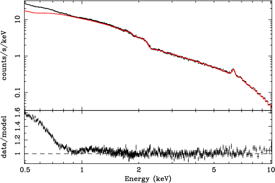
Figure 2: The $0.5-10.0{\rm\thinspace keV}$ spectrum of NGC 4593 fit with the photoabsorbed power-law from Fig. 1 and two Gaussians to model the iron lines. Note the clear evidence for a soft excess, possibly complicated by absorption features from a “warm absorber” within NGC 4593. For this fit, $\chi^{2}/{\rm dof}=11423/1736(6.58)$.

As a first, purely phenomenalogical attempt to describe the soft excess component, we have employed a single temperature thermal bremsstrahlung emission model (zbremss). To adequately describe the spectrum, we were required to include two warm absorbing zones as well as an iron-L₃ edge from iron atoms in line-of-sight dust. A natural interpretation is that the WA has distinct components at physically different distances from the central engine. We note that attempting to add a third zone into the model results in no statistical improvement in fit. Including this absorption structure provides a good description of the data ($\chi^{2}=1813/1745$; Fig. 3 and Table 1). We shall refer to this model as Model-1. The best fit value for the temperature characterizing this soft excess component is $kT\approx 0.21^{+0.003}_{-0.005}{\rm\thinspace keV}$ and it has a 0.5–10 keV flux of $2.01^{+0.33}_{-0.11}\times 10^{-14}\hbox{${\rm\thinspace erg}{\rm\thinspace cm}^{-2}{\rm\thinspace s}^{-1}\,$}$.

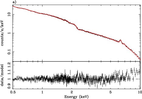
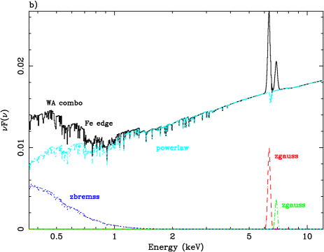
Figure 3: (a) The best fit for Model 1, including a zbremss component to represent the soft emission: $\chi^{2}/{\rm dof}=1813/1745(1.04)$. (b) The relative strength of the model components for Model 1. The $6.4$ and $6.97{\rm\thinspace keV}$ Gaussians are shown in red and green, respectively. The zbremss soft emission is in dark blue, and the photoabsorbed power-law is in light blue. Other absorption components are indicated in black.

Of course, the description of the soft excess in Model-1 is purely phenomenalogical in nature. Ideally, we would like to describe the soft excess with a model that has a direct physical interpretation. Initially, we attempt to describe the soft excess as soft X-ray reflection from a mildly-ionized accretion disk (see Brenneman & Reynolds 2006 for a successful application of this model to the Seyfert galaxy MCG-6-30-15). Operationally, we replace the thermal bremsstrahlung component in Model 1 with the ionized disk model reflion created by Ross & Fabian (2005). Because the irradiated matter is also responsible for producing the Fe-K$\alpha$ line in many sources, this model has the potential advantage of self-consistently describing the soft excess as well as the 6.4 keV emission line feature.

Interestingly, we find that we cannot successfully describe both the soft emission and the Fe-K$\alpha$ line with the disk reflection model. The resulting best fit is $\chi^{2}/{\rm dof}=2652/1745(1.52)$, and we found that significant residuals remained on the soft and hard ends of the spectra. Even adding the Gaussian component back to explicitly model the $6.4{\rm\thinspace keV}$ iron line (and hence removing the constraint that the disk reflection must describe this feature), the disk reflection model was unable to adequately fit the form of the soft excess. We thus conclude that ionized disk reflection is not an important process in shaping the soft X-ray spectrum of NGC 4593. Given the relative narrowness of the Fe-K$\alpha$ line in this source we believe it is not originating in the inner disk, and hence the above is not a surprising conclusion.

Alternatively, we can postulate that the soft excess is due to thermal Comptonization by plasma at a temperature between that of the disk and the hard X-ray corona (possibly in a transition zone). Operationally, we use the comptt model (Titarchuk 1994) to model the soft excess. Hereafter, we shall refer to this spectral model as Model 2. This preserves the physical realism of the soft emission arising from the accretion disk, but allows the iron line to be produced elsewhere, perhaps farther away in the molecular torus where it would not be as broad by nature. Model 2 reaches a best fit of $\chi^{2}/{\rm dof}=1759/1744(1.01)$. The best fit and model for Model 2 is shown in Fig. 4. Here we have frozen the seed photon temperature at $T_{0}=50{\rm\thinspace eV}$ and have kept a slab geometry for the corona. The best fit Comptonizing plasma temperature is $kT_{\rm c}=42{\rm\thinspace keV}$ with an optical depth of $\tau=0.12$, though both parameters were not very well constrained by the fit. This is not surprising, given that both are equally involved in shaping the spectrum via the Compton-y parameter: $y\propto\tau T_{\rm c}$. We note that for Model 2 the equivalent widths of the $6.4$ and $6.97{\rm\thinspace keV}$ Gaussians remain approximately unchanged from their values in the Model 1 fit.

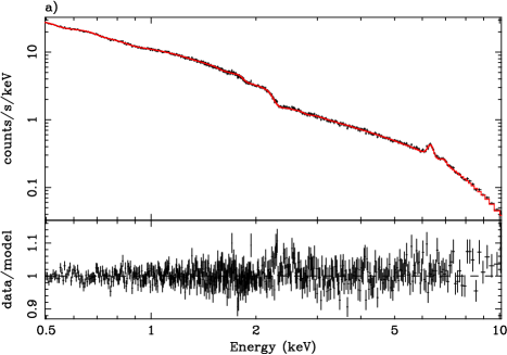
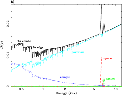
Figure 4: (a) The best fit for Model 2, including a comptt component to represent the soft emission in place of the zbremss component of Model 1. $\chi^{2}/{\rm dof}=1808/1744$. (b) The relative strength of the model components for Model 2. The color scheme is the same as in Fig. 3b.

Table 1 reports the parameter values and goodness of fit for both the final best fitting phenomenalogical model (Model 1, with zbremss and including all other components added in), and the more physical model (Model 2, including comptt and all other components). Using the Model 2 fit from Table 1, the total $0.5-10{\rm\thinspace keV}$ flux is $F_{\rm X}=6.74\times 10^{-11}\hbox{${\rm\thinspace erg}{\rm\thinspace cm}^{-2}{\rm\thinspace s}^{-1}\,$}$. Assuming a flat universe WMAP cosmology, this corresponds to a luminosity of $L_{\rm X}=1.21\times 10^{43}\hbox{${\rm\thinspace erg}{\rm\thinspace s}^{-1}\,$}$. Considering only the energy range from $2-10{\rm\thinspace keV}$, $L_{2-10}=7.40\times 10^{42}\hbox{${\rm\thinspace erg}{\rm\thinspace s}^{-1}\,$}$. This is roughly $21\%$ greater than the $2-10{\rm\thinspace keV}$ luminosity observed by McKernan et al. (2003), but only about $86\%$ of the value from the ASCA observation reported by Reynolds (1997).

The warm absorber modeled with our two created xstar tables suggests a multi-zone structure in column density and ionization, as discussed above. Though our model does not parameterize the covering fraction of the absorbing gas, we can approximate this fraction by representing the warm absorber with the O vii and O viii edges at $0.74$ and $0.87{\rm\thinspace keV}$, respectively, as has been done by many other authors examining warm absorbers (e.g., Reynolds 1997; McKernan et al. 2003). In so doing, we find that to $90\%$ confidence, the O vii edge has an optical depth of $\tau=0.16^{+0.02}_{-0.01}$ whereas the O viii edge is much less prominent at $\tau<0.01$. We therefore chose to use the O vii edge as a diagnostic for determining the covering fraction of the absorbing gas in NGC 4593. If the O vii edge accounts for the absorption by this gas, the photons absorbed should be reprocessed and radiated in emission as the O vii radiative recombination line at $0.574{\rm\thinspace keV}$. Assuming that this line will be narrow, we fit a Gaussian to the data. Adding in this component bettered the overall goodness-of-fit by $\Delta\chi^{2}/\Delta{\rm dof}=-53/-1$ as compared to the two-edge model for the warm absorber, showing that this line is statistically robust. The O vii RRC line had an upper limit equivalent width of $EW<6.35{\rm\thinspace eV}$ and a flux of $2.82\times 10^{-4}\hbox{${\rm\thinspace ph}{\rm\thinspace cm}^{-2}{\rm\thinspace s}^{-1}\,$}$, such that the line contributed $\sim 7182$ total photons to the model over the total observation time. The O vii edge, by contrast, contributed $\sim 31991$ total photons. Taking the ratio of the reprocessed photons to the absorbed photons, we can estimate a covering fraction for the warm absorber: $f\approx 0.23$.

Table 1: Best fit parameters for the EPIC-pn spectrum

Model Component	Parameter	Model 1 Value	Model 2 Value
phabs	$N_{\rm H}$ (${\rm\thinspace cm}^{-2}\,$)	$1.97\times 10^{20}$	$1.97\times 10^{20}$
WA 1	$N_{\rm H1}$ (${\rm\thinspace cm}^{-2}\,$)	$1.64^{+0.07}_{-0.09}\times 10^{23}$	$9.29^{+1.46}_{-9.15}\times 10^{22}$
	log $\xi_{1}$ (${\rm\thinspace erg}{\rm\thinspace cm}{\rm\thinspace s}^{-1}\,$)	$2.54^{+0.03}_{-0.04}$	$2.75^{+0.12}_{-0.32}$
WA 2	$N_{\rm H2}$ (${\rm\thinspace cm}^{-2}\,$)	$2.47^{+0.31}_{-0.73}\times 10^{21}$	$1.13^{+1.21}_{-0.94}\times 10^{22}$
	log $\xi_{2}$ (${\rm\thinspace erg}{\rm\thinspace cm}^{-1}{\rm\thinspace s}^{-1}\,$)	$0.57^{+0.13}_{-0.17}$	$1.70^{+0.30}_{-0.59}$
Fe-L3 edge	log $N_{\rm Fe}(\hbox{${\rm\thinspace cm}^{-2}\,$})$	$16.81^{+0.02}_{-0.05}$	$16.92^{+0.04}_{-0.08}$
po	$\Gamma$	$1.87\pm 0.004$	$1.75^{+0.02}_{-0.03}$
	flux (${\rm\thinspace erg}{\rm\thinspace cm}^{-2}{\rm\thinspace s}^{-1}\,$)	$5.11^{+0.04}_{-0.02}\times 10^{-13}$	$4.44^{+0.41}_{-0.54}\times 10^{-13}$
zgauss	$E({\rm\thinspace keV})$	$6.4$	$6.4$
	$\sigma({\rm\thinspace keV})$	$0.10\pm 0.08$	$0.10\pm 0.01$
	flux $(\hbox{${\rm\thinspace erg}{\rm\thinspace cm}^{-2}{\rm\thinspace s}^{-1}\,$})$	$4.46\pm 0.32\times 10^{-15}$	$4.15^{+0.33}_{-0.34}\times 10^{-15}$
	$E({\rm\thinspace keV})$	$6.97$	$6.97$
	$\sigma({\rm\thinspace keV})$	$0.10\pm 0.02$	$0.10\pm 0.06$
	flux $(\hbox{${\rm\thinspace erg}{\rm\thinspace cm}^{-2}{\rm\thinspace s}^{-1}\,$})$	$9.47^{+2.00}_{-2.07}\times 10^{-16}$	$7.77^{+2.07}_{-2.37}\times 10^{-16}$
zbremss	$kT({\rm\thinspace keV})$	$0.21^{+0.003}_{-0.005}$
	flux $(\hbox{${\rm\thinspace erg}{\rm\thinspace cm}^{-2}{\rm\thinspace s}^{-1}\,$})$	$2.01^{+0.33}_{-0.11}\times 10^{-14}$
comptt	$T_{0}({\rm\thinspace keV})$		$0.05$
	$kT({\rm\thinspace keV})$		$42.19^{+140.67}_{-40.19}$
	$\tau_{\rm p}$		$0.12^{+0.06}_{-0.11}$
	flux (${\rm\thinspace erg}{\rm\thinspace cm}^{-2}{\rm\thinspace s}^{-1}\,$)		$6.46^{+0.90}_{-0.92}\times 10^{-14}$
$\chi^{2}/{\rm dof}$		$1813/1745(1.04)$	$1759/1744(1.01)$

The energy range from $0.5-10.0{\rm\thinspace keV}$ is considered for the EPIC-pn. Best fit Model 1 contains a zbremss component to parameterize the soft excess below $\sim 2{\rm\thinspace keV}$, while best fit Model 2 represents this component with a comptt model. All quoted error bars are at the $90\%$ confidence level. All redshifts used were frozen at the cosmological value for NGC 4593: $z=0.009$.

4 Variable Nature of the Source

NGC 4593 displays significant variability (over a factor of two in $0.5-10{\rm\thinspace keV}$ flux) during the course of this observation. In this Section, we examine the detailed variability properties of this source.

4.1 Spectral Variability

We have analyzed the spectral variability of the source as seen in the EPIC-pn data. As an initial assessment of spectral variability, Fig. 5 plots the data-to-model ratios of consecutive $10{\rm\thinspace ks}$ segments of the EPIC-pn data using the comptt best fit spectrum model discussed in §3. Experimentation suggested that intervals smaller than $10{\rm\thinspace ks}$ contain insufficient counts to maintain the integrity of the spectrum. As well as the obvious variations in the normalization of the spectrum, there are clear changes in slope between segments (with the source becoming softer as it brightens). There is also a feature of variable equivalent width seen at $\sim 6.4{\rm\thinspace keV}$, corresponding to the cold Fe-K$\alpha$ line. Interestingly, though, we see no variable discrete features in the soft X-ray spectrum suggesting that there is no significant warm absorber variability during our observations.

To examine variability of the iron lines in more detail, Fig. 6 plots the renormalized interval data over the time-averaged data from $2-10{\rm\thinspace keV}$. Direct spectral fitting of the the cold and ionized Fe-K lines in each interval with Gaussian profiles illuminates the nature of their variability (or lack thereof). As can be seen in Table 2 and Figs. 7, the cold line exhibits an approximately constant flux and a variable equivalent width. The constant equivalent width hypothesis is rejected with greater than 99% significance, whereas a constant flux hypothesis is consistent with the data at the 20% level. Thus the evidence suggests that the cold iron line flux does not appear to respond to changes in the X-ray continuum. Constraints on the ionized line are not strong enough to rule out either a constant flux and equivalent width, as is shown in Fig. 8 and Table 2.

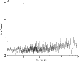
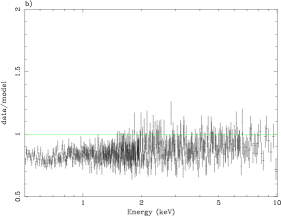
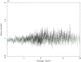
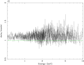
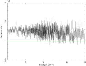
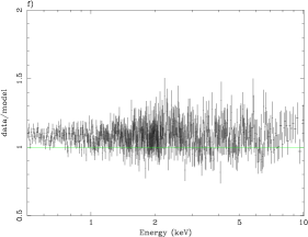
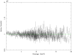
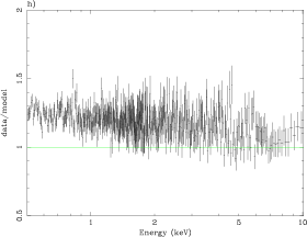
Figure 5: Variation of the EPIC-pn time-averaged spectrum from the comptt best fit model discussed in §3. Time intervals are $10{\rm\thinspace ks}$ in length except for the last, which is $\sim 6100{\rm\thinspace ks}$. Segments a) - h) are shown in chronological order of the observation.

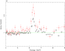
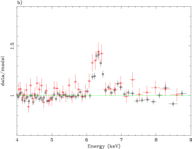
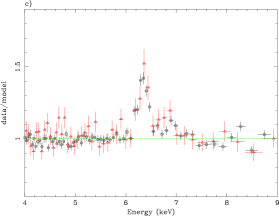
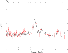
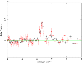
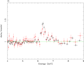
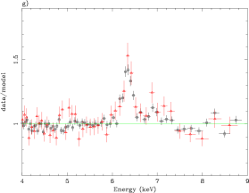
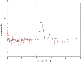
Figure 6: The cold and ionized Fe-K$\alpha$ lines from the time-separated EPIC-pn spectrum. Time intervals are $10{\rm\thinspace ks}$ each in length, as above in Fig. 5. Lines are above a phabs po continuum. The time-averaged data appear in black squares, interval data in red triangles.

Table 2: The cold and ionized iron lines in the EPIC-pn spectrum of NGC 4593

Line	FWHM (${\rm\thinspace km}{\rm\thinspace s}^{-1}\,$)	Flux (${\rm\thinspace erg}{\rm\thinspace cm}^{-2}{\rm\thinspace s}^{-1}\,$)	EW (${\rm\thinspace eV}$)
Cold Fe-K$\alpha$	$13245\pm 2208$	$7.41\pm 0.86\times 10^{-13}$	$232\pm 27$
($6.40{\rm\thinspace keV}$)	$8831\pm 2208$	$4.98\pm 0.89\times 10^{-13}$	$126\pm 22$
	$9934\pm 2208$	$5.76\pm 0.85\times 10^{-13}$	$134\pm 19.8$
	$13246\pm 3311$	$7.26\pm 1.04\times 10^{-13}$	$153\pm 21.8$
	$8831\pm 2208$	$5.27\pm 0.86\times 10^{-13}$	$105\pm 17.2$
	$11038\pm 4415$	$4.08\pm 0.93\times 10^{-13}$	$88.5\pm 20.2$
	$8831\pm 2208$	$5.61\pm 0.88\times 10^{-13}$	$137\pm 21.5$
	$11038\pm 3311$	$5.82\pm 1.17\times 10^{-13}$	$124\pm 24.9$
Ionized Fe-K$\alpha$	$7095\pm 6081$	$1.97\pm 1.41\times 10^{-13}$	$64.3\pm 46.0$
($6.97{\rm\thinspace keV}$)	$50678\pm 83111$	$2.89\pm 5.05\times 10^{-13}$	$80.3\pm 140$
	$6081\pm 6081$	$2.09\pm 1.54\times 10^{-13}$	$51.9\pm 38.3$
	$14190\pm 11149$	$2.04\pm 2.22\times 10^{-13}$	$45.6\pm 49.6$
	$9122\pm 6081$	$2.52\pm 1.85\times 10^{-13}$	$53.7\pm 39.4$
	$18244\pm 9122$	$3.06\pm 3.48\times 10^{-13}$	$71.3\pm 57.8$
	$24325\pm 9122$	$4.90\pm 3.00\times 10^{-13}$	$132\pm 80.9$
	——-	——-	——-

Each row represents a time interval of $10{\rm\thinspace ks}$ in the observation. Fits were done in xspec using a phabs po model for the continuum and two Gaussian lines with parameters fit to the data in each time interval. Error bars are at $1\sigma$. The blank lines in the ionized Fe-K$\alpha$ table represent time intervals for which a robust fit to the data could not be achieved.

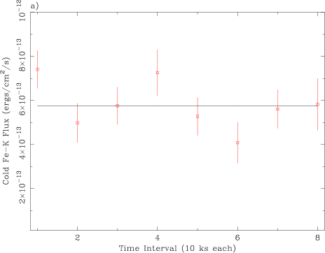
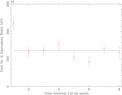
Figure 7: Variation of the flux (a) and equivalent width (b) of the cold Fe-K$\alpha$ line ($6.4{\rm\thinspace keV}$) in $10{\rm\thinspace ks}$ intervals over the course of the $76{\rm\thinspace ks}$ observation. A fit to the data with a constant flux model yields $\chi^{2}/{\rm dof}=10/7$ ($1.43$) implying a 20% probability that the data are consistent with the constant flux model. The constant equivalent width fit yields $\chi^{2}/{\rm dof}=22/7$ ($3.14$) allowing the constant equivalent width hypothesis to be rejected at more than the 99% significance level.

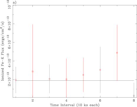
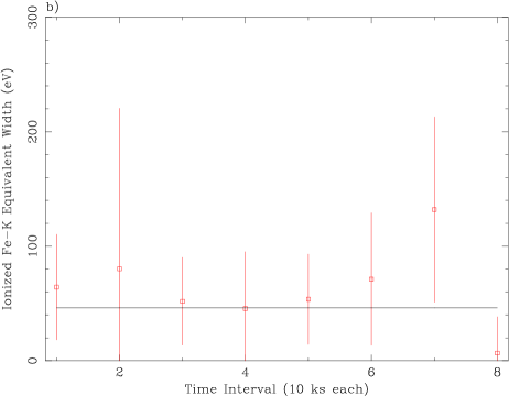
Figure 8: Variation of the flux (a) and equivalent width (b) of the ionized Fe-K$\alpha$ line ($6.97{\rm\thinspace keV}$) over the course of the observation. Here the uncertainty in the data is so great that a constant flux cannot be ruled out: $\chi^{2}/{\rm dof}=3/7$ ($0.43$). A constant equivalent width is similarly likely: $\chi^{2}/{\rm dof}=3/7$ ($0.43$).

The simplest way to interpret the lack of continuum response of the cold iron line is to suppose that it exists on spatial scales with light travel times greater than the duration of our observation. For an observation time of $76{\rm\thinspace ks}$, as is the case here, the light would travel approximately $150$ AU, or roughly $1.9\times 10^{3}\,r_{g}$ if NGC 4593 harbors a $8.1\times 10^{6}\hbox{$\rm\thinspace M_{\odot}$}$ black hole at its core (see discussion at the end of §4.2). The lack of response for the iron line flux would suggest that this size is a lower limit for the size of the line emitting source. This would place the line emission in the outer regions of the accretion disk or the putative molecular torus of the Seyfert unification scheme.

4.2 Continuum Power Spectrum and Spectral Lags

The light curve for the full-band (0.5-10.0  keV) data set is shown in Fig. 9a. The light curve is characterized by an initial rapid drop up to $\sim 5{\rm\thinspace ks}$, followed by a relatively steady increase peaking at $\sim 45{\rm\thinspace ks}$, a drop until $\sim 65{\rm\thinspace ks}$, and then a final increase that shows possible signs of tapering off around the end of the observation at $76{\rm\thinspace ks}$. There are indications of smaller scale variability on time scales of $<1000{\rm\thinspace s}$, with slight flares and drops occurring throughout the data set.

Fig. 9b shows the Leahy normalized power spectrum of the $0.5-10{\rm\thinspace keV}$ EPIC-pn light curve. The power spectrum demonstrates that the variability of the source becomes dominated by Poisson statistics on timescales of about $200{\rm\thinspace s}$ once it drops to a power of $\sim 2$, as expected. Before this point, the slope of the power spectrum for low frequencies is $-2.63^{+0.66}_{-0.25}$. This value for the PSD slope is consistent with results from several other Sy-1 AGN such as NGC 3783 (Markowitz 2005), MCG–6-30-15 (Papadakis et al. 2005; Vaughan et al. 2003), NGC 4051 (at high frequencies; McHardy et al. 2004), and Mrk 766 (also at high frequencies; Vaughan & Fabian 2003).

Given the range of X-ray energies available in this dataset, it is also useful to study the continuum variability in different energy bands. Hardness ratios and time lags between different energy bands in the continuum, in particular, can help constrain the emission mechanisms of the source as well as the physical scale of the emitting region(s). We divide the X-ray spectrum into three energy bands, each with an approximately equal number of counts ($\sim 5\times 10^{5}$). The soft band ranges from $0.5-0.84{\rm\thinspace keV}$, the mid band extends from $0.84-1.5{\rm\thinspace keV}$, and the hard band covers $1.5-10.0{\rm\thinspace keV}$. The light curves for all three bands are represented in Fig. 10. In order to test whether a time lag exists between these energy bands, we compute the cross-correlation function between the three energy bands using the xronos package (Stella & Angelini 1991) as well as the discrete correlation function (DCF; Edelson & Krolik 1988). We measured the hard-to-soft band lag to be $230\pm 50{\rm\thinspace s}$ (i.e., the hard band lags the soft band by this amount of time; Fig. 11).

Figure 9: The light curve (a) and power spectrum (b) for the time-averaged pn data from NGC 4593. Variations on timescales as small as hundreds of seconds appear visible in the source. Note that the frequency at which the power spectrum flattens into Poisson noise is about $5\times 10^{-3}{\rm\thinspace Hz}$. Inverting this means that the smallest timescale of variability we can reliably observe from this source is $\sim 200{\rm\thinspace s}$. At low frequencies, the slope of the power spectral density curve is $-2.63^{+0.66}_{-0.25}$.

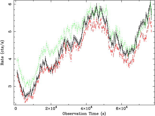
Figure 10: Light curves for the different energy bands: the soft band runs from $0.5-0.84{\rm\thinspace keV}$ (solid black), the mid band runs from $0.84-1.5{\rm\thinspace keV}$ (dashed red), and the hard band runs from $1.5-10.0{\rm\thinspace keV}$ (dotted green).

The most straightforward interpretation of these time delays envisions them as representing the finite scattering time within the Comptonizing disk-corona system that is thought to be responsible for the primary X-ray production. One should be cautioned, however, that this interpretation invokes numerous underlying simplifications with regard to the physical mechanism that produces these types of time lags between energy bands. See Pottschmidt et al. (2003) and Nowak et al. (1999, 2002) for more detailed accounts of other factors that can be responsible for or affect the observed time lag between the hard and soft energy bands. We assume here that both the hard and soft X-ray photons originate from seed UV photons from the disk, which are then Comptonized by a corona of relativistic electrons surrounding the disk. The energy of a given photon in our simplified scheme will thus depend on the number of scatterings it undergoes with the electrons, and one may therefore infer that the more energetic photons have experienced more interactions. It is thus possible to estimate the size of the coronal region by measuring the time lag between the peaks of the hard and soft photon light curves of the source, as we have done, and making the simplified assumption that the corona possesses a slab or spherical geometry. With each scattering, a seed photon gains on average a fractional energy $\Delta E/E\approx 4k_{B}T/m_{e}c^{2}$, where $T$ is the temperature of the electrons in the corona. So the energy of a Comptonized photon after a given number of scatterings will be:

$$E\approx E_{0}\left(1+\frac{4k_{B}T}{m_{e}c^{2}}\right)^{n}$$ (2)

where $E_{0}$ is the initial seed photon energy and $n$ is the number of scatterings (Rybicki & Lightman 1979; Chiang et al. 2000). The time delay of this photon relative to the seed photon source will be roughly proportional to the number of scatterings, $t\approx nt_{0}$. Here $t_{0}\sim l_{T}/c$ where $l_{T}$ is the mean free path for Thomson scattering in an optically-thick corona or, if the corona is optically-thin, simply the size of the corona. We take the effective photon energy in the soft range ($0.5-0.84{\rm\thinspace keV}$) to be $0.67{\rm\thinspace keV}$. For the hard range ($1.5-10{\rm\thinspace keV}$) we calculate the effective photon energy to be $2.17{\rm\thinspace keV}$. Both estimates are based on taking weighted averages (based on flux) of the energies in the soft and hard ranges, and accounting for the energy-dependent effective area of the pn. Assuming that the energy of the coronal electrons ranges from $50-100{\rm\thinspace keV}$, our measured soft-hard time lag of $\sim 226{\rm\thinspace s}$ suggests that the corona occupies a region around the disk $1.91-3.34\times 10^{12}{\rm\thinspace cm}$ in size. This is derived assuming the size of the corona is given by

$$r\approx tc\frac{\log\left(1+\frac{4k_{\rm B}T}{m_{\rm e}c^{2}}\right)}{\log\frac{E}{E_{\rm 0}}}$$ (3)

We will assume that the central black hole in NGC 4593 has a mass of $8.1\times 10^{6}\hbox{$\rm\thinspace M_{\odot}$}$ based on reverberation mapping (Nelson & Whittle 1995; Gebhardt et al. 2000). Using this mass for the NGC 4593 black hole, the characteristic length scale of the corona would be in the range of $1.6-2.8r_{\rm g}$.

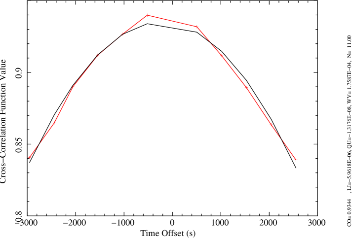
Figure 11: The cross-correlation function for the soft-to-hard energy bands in NGC 4593 in red (with data points), plotted with the best fit curve in solid black. The vertical line represents a zero time delay between the two bands; the off-centeredness of the curve peak indicates that the hard band lags the soft band by $226\pm 53{\rm\thinspace s}$ at $90\%$ confidence.

5 Discussion and Conclusions

5.1 Summary of Results

We have obtained a $76{\rm\thinspace ks}$ XMM-Newton observation of the Sy-1 galaxy NGC 4593. An examination of the best fitting EPIC-pn spectrum shows that the continuum is well modeled by a photoabsorbed power-law with $N_{\rm H}=1.97\times 10^{20}\hbox{${\rm\thinspace cm}^{-2}\,$}$, $\Gamma=1.75$, and a flux of $4.44\times 10^{-13}\hbox{${\rm\thinspace erg}{\rm\thinspace cm}^{-2}{\rm\thinspace s}^{-1}\,$}$. The best fit to the hard spectrum can be achieved by including two Gaussian emission lines representing cold and ionized fluorescent iron at $6.4$ and $6.97{\rm\thinspace keV}$, respectively.

We see clear evidence for a complex warm absorber in the EPIC-pn spectrum. Fitting a grid of photoionization models computed using the xstar code, we infer a warm absorber with two physically and kinematically distinct zones: one with a column density of $N_{\rm H}=9.29\times 10^{22}\hbox{${\rm\thinspace cm}^{-2}\,$}$ and an ionization parameter of $\log\xi=2.75$, the other with $N_{\rm H}=1.13\times 10^{22}\hbox{${\rm\thinspace cm}^{-2}\,$}$ and $\log\xi=1.70$, which is likely more distant from the central engine. We robustly detect the L₃ edge of neutral iron presumed to exist in the form of dust grains along the line-of-sight to the central engine, as cited by McKernan et al. (2003). This edge has a column density of $N_{\rm Fe}=8.32\times 10^{16}\hbox{${\rm\thinspace cm}^{-2}\,$}$.

A soft excess below $\sim 2{\rm\thinspace keV}$ is also seen in the data, and can be accounted for either phenomenalogically by a redshifted bremsstrahlung component (Model 1) or, more effectively and physically, a component of Comptonized emission from an accretion disk of seed photons upscattered by a plasma of relativistic electrons existing in either a corona or the base of a jet near the disk in some geometry (Model 2). The latter scenario yields the best statistical fit to the data, with a seed photon temperature of $T_{\rm 0}=50{\rm\thinspace eV}$, an electron temperature of $kT=42{\rm\thinspace keV}$, a plasma optical depth of $\tau_{\rm p}=0.12$ and a flux of $6.46\times 10^{-14}\hbox{${\rm\thinspace erg}{\rm\thinspace cm}^{-2}{\rm\thinspace s}^{-1}\,$}$.

Lastly, cold and ionized Fe-K emission lines were wanted by the fit at $6.4$ and $6.97{\rm\thinspace keV}$, respectively. The cold line Gaussian had a time-averaged equivalent width of $EW=131{\rm\thinspace eV}$, while the ionized component had an $EW=45{\rm\thinspace eV}$. Although the continuum varied with time over the course of our observation, the flux of the cold Fe-K$\alpha$ showed marginal evidence for variability between successive $10{\rm\thinspace ks}$ intervals. The equivalent width of this line, on the other hand, is shown to vary significantly. The simplest interpretation of this result is to suppose that the cold line originates from a region with a light-crossing time larger that the length of our observation. For a black hole mass of $8.1\times 10^{6}\hbox{$\rm\thinspace M_{\odot}$}$, this places the cold line emitting region beyond about $2000r_{g}$ from the black hole, i.e., in the outer accretion disk or the putative molecular torus of Seyfert unification schemes. Our statistics on the ionized Fe-K line are insufficient to constrain its variability properties — these data are consistent with both constant flux and constant equivalent width.

We have detected a $226{\rm\thinspace s}$ time-lag between the hard and soft EPIC-pn bands, with the hard band lagging the soft. In a simple model in which this corresponds to scattering times within a Comptonizing corona, we conclude that the corona can only possess a size of $\sim 1.6-2.8r_{\rm g}$.

5.2 Implications for the X-ray Emission Region

The narrowness of the fluorescent iron line together with the lack of response of this line to changes in the hard X-ray continuum suggest an absence of a cold, optically-thick matter within the central $\sim 10^{3}r_{g}$ of the accretion disk. The standard framework for accommodating such a result is to postulate that the inner regions ($r\lesssim 10^{3}r_{\rm g}$) of the accretion flow have entered into a radiatively-inefficient mode which is extremely hot (electron temperatures of $T\sim 10^{10}{\rm\thinspace K}$), optically-thin, and geometrically-thick (e.g., Rees 1982; Narayan & Yi 1994). Within this framework, the hard X-ray source is identified as thermal bremsstrahlung or Comptonization from this structure. However, the variability of the X-ray continuum is inconsistent with X-ray emission from a structure which is $\sim 1000r_{\rm g}$ in extent. The rapid continuum variability and the short time lag between the hard and soft X-ray photons dictate that, at any given time, the X-ray emission region is only $\sim 1-3r_{\rm g}$ in extent.

We are therefore led to consider alternative geometries and/or origins for the X-ray source. We consider three possibilities. Firstly, the inner accretion flow may indeed be radiatively-inefficient, but the observed X-ray emission may come from the compact base of a relativistic jet powered by black hole spin. Secondly, the X-ray emission may indeed originate from the body of the radiately-inefficient flow but, at any given instant in time, be dominated by very compact emission regions within the flow. Such emission regions may be arise naturally from the turbulent flow or, instead, may be related to a magnetic interaction between the inner parts of the flow and the central spinning black hole (Wilms et al. 2001; Ye et al. 2007). In this case the iron line could still plausibly originate at a distance of thousands of $r_{\rm g}$ and thus be quite narrow. Finally, it is possible that the accretion disk is radiatively-efficient (and hence optically-thick and geometrically-thin) close to the black hole and supports a compact accretion disk corona. Of course, an immediate objection to this scenario is the lack of a broadened iron line. However, as demonstrated in R04, it is possible the iron line is so broad that it is buried in the noise of the continuum. Alternatively, the accretion disk surface may have an ionization state such that iron line photons are effectively trapped by resonant scattering and destroyed by the Auger effect. Longer observations with better spectral and timing resolution will be necessary in order to confirm our results and differentiate between these different possible scenarios.

5.3 Conclusions

We have shown that the Sy-1 galaxy NGC 4593 has a continuum spectrum that is fit remarkably well by a simple photoabsorbed power-law above $\sim 2{\rm\thinspace keV}$. Below this energy, we see evidence for spectral complexity that can be attributed to the presence of a possible multi-zone layer of absorbing material intrinsic to the source, as well as a soft excess that cannot be explained by a reflection model from an ionized disk. Also arguing against a disk-reflection-dominated source is that unlike other sources of its kind (e.g., MCG–6-30-15), NGC 4593 has relatively narrow cold and ionized Fe-K$\alpha$ line features at $6.4$ and $6.97{\rm\thinspace keV}$, respectively. See R04 for a more thorough discussion of these lines and their possible physical interpretations. We can say that the cold line is most likely formed either quite far out in the accretion disk, or possibly in the putative dusty torus region surrounding the central engine, based on their narrowness and lack of significant variability over the $76{\rm\thinspace ks}$ duration of our observation. We find no evidence for reflection features from the inner accretion disk (e.g., a “broad iron line”) in the spectrum.

Based on the time lag between the soft and hard spectral bands, we estimate that the corona occupies the a region around the central source on the order of $\sim 1.6-2.8r_{\rm g}$, assuming that NGC 4593 harbors a $8.1\times 10^{6}\hbox{$\rm\thinspace M_{\odot}$}$ black hole at its core and that the energies of the electrons in the corona range from $\sim 50-100{\rm\thinspace keV}$. This estimate for the coronal size is reinforced by our measurements of continuum variability on timescales as small as $\sim 200{\rm\thinspace s}$, equivalent to a light travel time of $\sim 4r_{\rm g}$ for the black hole mass in question.

Taken together, the implications of a narrow iron line emitted far out in the disk or torus and the small coronal size in NGC 4593 present an atypical picture of an AGN. We postulate that the primary X-ray source is associated with the compact base of a jet or compact emission regions within a much larger optically-thin accretion flow. Alternatively, the accretion disk may be radiatively-efficient with a compact corona but not display a broad iron line due to the effects of extreme broadening or disk ionization.

References

- (1) Anders E. & Grevesse, N., 1989, Geo. Cosm. Acta, 53, 197.
- (2) Arnaud K.A., 1996, ASP Conf. Series, 101, 17.
- (3) Awaki H. et al. , 2005, Astrophys. J., 632, 793.
- (4) Balucinska-Church M. & McCammon D., 1992, Astrophys. J., 400, 699.
- (5) Basko M.M., 1978, Astrophys. J., 223, 268.
- (6) Chiang J. et al. , 2000, Astrophys. J., 528, 292.
- (7) Edelson R.A. & Krolik J.H., 1988, Astrophys. J., 333, 646.
- (8) Elvis M., Wilkes B.J., & Lockman F.J., 1989, Astr. J., 97, 777.
- (9) Fabian A.C. et al. , 1989, Mon. Not. R. astr. Soc., 238, 729.
- (10) Ferrarese L. & Merritt, D., 2000, Astrophys. J., 539, L9.
- (11) Gebhardt K. et al. , 2000, Astrophys. J., 543, L5.
- (12) George I.M. & Fabian A.C., 1991, Mon. Not. R. astr. Soc., 249, 352.
- (13) Guilbert P.W. & Rees M.J., 1988, Mon. Not. R. astr. Soc., 233, 475.
- (14) Halpern J.P., 1984, Astrophys. J., 281, 90.
- (15) Kaastra J.S., Steenbrugge K.C., 2001, JHU/LHEA Workshop.
- (16) Kallman T.R. & Krolik J.H., 1995, XSTAR Manual, available at legacy.gsfc.nasa.gov.
- (17) Kirsch M.G. et al. , 2005, SPIE, 5898, 22.
- (18) Laor A., 1991, Astrophys. J., 376, 90.
- (19) Lewis D.W., MacAlpine G.M., & Koski A.T. 1978, Bull. Amer. Astron. Soc., 10, 388.
- (20) Lightman A.P. & White T.R., 1988, Astrophys. J., 335, 57.
- (21) Lynden-Bell D., 1969, Nature, 223, 690.
- (22) Markowitz A., 2005, Astrophys. J., 635, 180.
- (23) Matt G., Perola G.C., Piro L., 1991, Astr. Astrophys., 245, 63.
- (24) McHardy I.M. et al. , 2004, Mon. Not. R. astr. Soc., 348, 783.
- (25) McKernan B. et al. , 2003, Astrophys. J., 593, 142.
- (26) Nandra K. et al. , 1997a, Astrophys. J., 477, 602.
- (27) Narayan R. & Yi I., 1994, Astrophys. J., 428L, 13.
- (28) Nelson C. & Whittle, M., 1995, Astrophys. J. Suppl., 99, 67.
- (29) Nowak M.A. et al. , 1999, Astrophys. J., 515, 726.
- (30) Nowak M.A. et al. , 2002, Mon. Not. R. astr. Soc., 332, 856.
- (31) Papadakis I.E., Kazanas D. & Akylas A., 2005, Astrophys. J., 631, 727.
- (32) Pottschmidt K. et al. , 2003, Astr. Astrophys., 407, 1039.
- (33) Pounds K.A. & Turner, T.J., 1988, Soc. Astr. Ital. Mem., 59, 261.
- (34) Rees M.J., 1982, Amer. Inst. Phys. Conf., 83, 166.
- (35) Reynolds C.S., 1997, Mon. Not. R. astr. Soc., 286, 513.
- (36) Reynolds C.S., 2000, Astrophys. J., 533, 811.
- (37) Reynolss C.S. et al. , 2004, Mon. Not. R. astr. Soc., 352, 205.
- (38) Reynolds C.S., Nowak M.A., 2003, Phys. Reports, 377, 389.
- (39) Reynolds C.S., Wilms J., 2004, Mon. Not. R. astr. Soc., 349, 1153.
- (40) Ross R.R. & Fabian A.C., 2005, Mon. Not. R. astr. Soc., 358, 211.
- (41) Rybicki G.B. & Lightman, A.P., 1979, Radiative Processes in Astrophysics (New York: Wiley).
- (42) Salpeter E.E., 1964, Astrophys. J., 140, 796.
- (43) Stella L. & Angelini L., 1991, ASP Conf. Series, 35, 103.
- (44) Vaughan S. & Fabian A.C., 2003, Mon. Not. R. astr. Soc., 341, 496.
- (45) Vaughan S., Fabian A.C. & Nandra K., 2003, Mon. Not. R. astr. Soc., 339, 1237.
- (46) Weaver K.A., Gelbord J., & Yaqoob T. 2001, Astrophys. J., 550, 261.
- (47) Wilms J. et al. , 2001, Mon. Not. R. astr. Soc., 328, L27.
- (48) Ye Y.C., Wang D.X. & Ma R.Y., 2007, New Astr., in press (astroph/0701802).
- (49) Zel’Dovich Y.B., 1965, Astronom. Zhurnal, 42, 283.
- (50)