Flame Evolution During Type Ia Supernovae and the Deflagration Phase in the Gravitationally Confined Detonation Scenario

Abstract

We develop an improved method for tracking the nuclear flame during the deflagration phase of a Type Ia supernova, and apply it to study the variation in outcomes expected from the gravitationally confined detonation (GCD) paradigm. A simplified 3-stage burning model and a non-static ash state are integrated with an artificially thickened advection-diffusion-reaction (ADR) flame front in order to provide an accurate but highly efficient representation of the energy release and electron capture in and after the unresolvable flame. We demonstrate that both our ADR and energy release methods do not generate significant acoustic noise, as has been a problem with previous ADR-based schemes. We proceed to model aspects of the deflagration, particularly the role of buoyancy of the hot ash, and find that our methods are reasonably well-behaved with respect to numerical resolution. We show that if a detonation occurs in material swept up by the material ejected by the first rising bubble but gravitationally confined to the white dwarf (WD) surface (the GCD paradigm), the density structure of the WD at detonation is systematically correlated with the distance of the deflagration ignition point from the center of the star. Coupled to a suitably stochastic ignition process, this correlation may provide a plausible explanation for the variety of nickel masses seen in Type Ia Supernovae.

1. Introduction

It is widely believed that in a type Ia supernova explosion, a WD near the Chandrasekhar limiting mass is disrupted by a thermonuclear runaway in its interior, and more precisely that a subsonic deflagration must precede any detonation (see Hillebrandt & Niemeyer 2000 and references therein). The current leading paradigms for how the deflagration of a WD takes place, and how this leads to astrophysical properties that match observations, are generally termed (1) pure deflagration, (2) deflagration detonation transition (DDT), (3) pulsational detonation, and (4) gravitationally confined detonation (GCD, Plewa et al. 2004). In all but the first of these, a subsonic deflagration phase expands the WD, lowering its density, and a subsequent supersonic detonation then incinerates the remainder of the star. Among the remaining three, the process that is proposed to ignite the detonation is very different, though it is crucial to determine how much expansion can occur prior to the detonation in order to predict the variation of nickel mass and therefore brightness among the observed Type Ia’s.

A primary purpose of this work is to set out a numerically efficient method for modeling the nuclear energy release in the flame front that propagates via heat diffusion during the deflagration stage. This formalism will be used for studying a variety of features of all of the above paradigms in future work. Nucleosynthesis of species produced as a result of electron captures provides a very important observational constraint on supernova models, especially the pure-deflagration scenario. For this reason, and because methods are available in the literature (Gamezo et al., 2005), we have included electron capture and neutrino emission in the energetic treatment to capture its effect on the hydrodynamics. Description of this method incorporates our previous work (Calder et al., 2007) detailing the nuclear processing of $\mathrm{{}^{12}C}$ and $\mathrm{{}^{16}O}$ by a flame front and the evolution of the resulting ash. A method for integrating this simplified 3-stage energy release with an artificially broadened flame is described in Section 2. The acoustic properties of this method are discussed in Section 3, where it is shown that the front emits very little acoustic noise. This is important for reducing spurious seeding of the strong hydrodynamic instabilities present during the deflagration phase.

We have chosen in this work to initially pursue simulations of the deflagration phase in GCD because it provides a more direct demonstration of the buoyancy character of the flame bubble and current work on this mechanism (Plewa et al., 2004; Calder et al., 2004; Plewa, 2007; Röpke et al., 2006b) can benefit from a concise parameter study. In this mechanism, the strong eruption of a rising flame bubble through the surface creates a wave of material traveling over the surface that collides at the point opposite breakout, compressing and heating unburnt surface material until detonation conditions are reached. We therefore proceed in section 4 to discuss our setup for simulating the deflagration of the star, in which our principle hypothesis is that the first flame ignition point is rare and therefore the deflagration phase is dominated by a single flame bubble. Some perspective is given with respect the conditions expected to be present in the WD core at this time, and we describe the progression of the burning in the simulation, including a survey of the effects of simulation resolution. Finally, in section 5 we present the results of simulations in which the ignition point of the flame is placed at various distances from the center of the star. We find that the density of the star at the time when the GCD mechanism predicts an ignition of the detonation, and thus the mass that will be processed to Fe group elements, is well correlated with the offset of the initial ignition point. This parameter study also serves as a touch-point for future larger-scale simulations of this mechanism in three dimensions (Jordan et al., 2007), which are essential for judging its viability (Röpke et al., 2006b). We summarize and make some concluding remarks in section 6.

2. Burning Model for a Carbon Oxygen White Dwarf

There are two fairly different methods of flame-front tracking used in contemporary studies of WD deflagrations. Use of a front-tracking method is necessary because the physical thickness of the flame front is unresolvable in any full-star scale simulation, with the carbon consumption stage being $10^{-4}$ to $10^{3}$ cm thick for the density range important in the star (Calder et al., 2007). The method presented here is based upon propagating a reaction progress variable with an advection-reaction-diffusion (ADR) equation, and can be thought of as an artificially thickened flame, because the real flame is also based on reaction-diffusion on much smaller scales. This type of method has been used in many previous simulations of the WD deflagration, both in full star simulations (e.g. Gamezo et al. 2003; Calder et al. 2004; Plewa 2007) and to study the effect of the Rayleigh-Taylor (R-T) instability on a propagating flame front (Khokhlov, 1995; Zhang et al., 2007). Our flame propagation is based heavily on this work, and we have made several refinements to the method that we will describe in detail below. The other widely used method utilizes the level set technique (Smiljanovski et al., 1997; Reinecke et al., 1999; Röpke et al., 2003) and performs an interface reconstruction in each cell based upon the value of a smooth field defined on the grid and propagated with an advection equation acting in addition to the hydrodynamics. See Röpke et al. (2006b) and Schmidt et al. (2006) for recent deflagration simulations using this method.

It should be emphasized that the implementation of the flame propagation is far from the only difference between these approaches, and there is considerable latitude even within one of the front-tracking methods. In addition to the front-tracking itself two other issues are important. First, the energy release of the nuclear burning must be treated, and this is typically done in some simplified way for computational efficiency. For example, a prominent difference between the method presented here and that commonly used with level-set is that we include electron captures in the post-flame material within our treatment. The second important additional component is what measure is taken to prevent the breakdown of the flame tracking method when R-T, and possibly secondary instability in the induced flow, is strong enough to drive flame surface perturbations on a sub-grid scale. Both methods fail in this limit because the scalar field being used to propagate the flame is distorted by advection due to strong turbulence. Generally this has been overcome by increasing the flame speed enough to polish out grid-scale disorder in the flow field. This can, however, be phrased in terms of simple (Khokhlov, 1995) or complex (Schmidt et al., 2006) laws intended to mimic the enhanced flame surface area produced by unresolved structure in the flame. We will leave further discussion to separate work, but awareness of this difference is important for comparing results of the two methods.

2.1. ADR Flame-front Model

Generally, an ADR scheme characterizes the location of a flame front using a reaction progress variable, $\phi$, which increases monotonically across the front from 0 (fuel) to 1 (ash). Evolution of this progress variable is accomplished via an advection-diffusion-reaction equation of the form

$$\frac{\partial\phi}{\partial t}+\vec{v}\cdot\nabla\phi=\kappa\nabla^{2}\phi+\frac{1}{\tau}R(\phi)\ ,$$ (1)

where $\vec{v}$ is the local fluid velocity, and the reaction term, $R(\phi)$, timescale, $\tau$, and the diffusion constant, $\kappa$, are chosen so that the front propagates at the desired speed. Vladimirova et al. (2006) showed that the step-function reaction rate widely in use led to a substantial amount of unwanted acoustic noise. They studied a suitable alternative, the Kolmogorov Petrovski Piskunov (KPP) reaction term which has an extensive history in the study of reaction-diffusion equations. In the KPP model the reaction term is given by

$$R(\phi)=\frac{1}{4}\phi(1-\phi)\ .$$ (2)

The symmetric and low-order character of this function gives it very nice numerical properties, leading to amazingly little acoustic noise. Following Vladimirova et al. (2006), we adopt $\kappa\equiv sb\Delta x/16$ and $\tau\equiv b\Delta x/16s$, where $\Delta x$ is the grid spacing, $s$ is the desired propagation speed, and $b$ sets the desired front width scaled to represent approximately the number of zones.

The KPP reaction term, however, has two serious drawbacks. Formally, the flame speed is only single valued for initial conditions that are precisely zero (and stay that way) outside the burned region (Xin, 2000), which cannot really be effected in a hydrodynamics simulation. This can lead to an unbounded increase of the propagation speed, which is precisely the property we wish to have under good control. Secondly, the progress variable $\phi$ takes an infinite amount of time to actually reach 1 (complete consumption of fuel). While not a fatal flaw like the flame speed problem, this is a problem for our simulations in which we would like to have a localized flame front so that fully-burned ash can be treated as pure NSE material.

Both of these drawbacks can be ameliorated by a slight modification of the reaction term (Asida et al., 2007) to

$$R(\phi)=\frac{f}{4}(\phi-\epsilon_{0})(1-\phi+\epsilon_{1})\ ,$$ (3)

where $0<\epsilon_{0},\epsilon_{1}\ll 1$ and $f$ is an additional factor that depends on $\epsilon_{0}$ and $\epsilon_{1}$ and the flame width so that the flame speed is preserved with the same constants as for KPP above. This “sharpened” KPP (sKPP) has truncated tails in both directions (thus being sharpened), making the flame front fully localized, and is a bi-stable reaction rate and thus gives a unique flame speed (Xin, 2000). The price paid is that since $R(\phi)=0$ for $\phi\leq 0$ and $\phi\geq 1$, (3) is discontinuous, adding some noise to the solution. Since the suppression of the tails is stronger for higher $\epsilon_{0}$ and $\epsilon_{1}$, we adjusted $\epsilon_{0}$ and $\epsilon_{1}$ so that for a particular flame width we could meet our noise goals. The parameter values used in the simulations presented in this work were $\epsilon_{0}=\epsilon_{1}=10^{-3}$, $f=1.309$, and $b=3.2$. The noise properties of these choices are discussed in section 3.

Diffusive flames are known to be subject to a curvature effect that affects the flame speed when the radius of curvature is similar to the flame thickness, a frequent circumstance with modestly-resolved flame front structure. In testing, the curvature effect of the step-function reaction rate proved surprisingly strong, likely due to the exponential “nose” that the flame front possesses (Vladimirova et al., 2006). Both KPP and our sKPP show significantly better curvature properties. Due to the necessary discussion of background and the size of the study supporting this conclusion, this topic will be discussed in detail separately (Asida et al., 2007).

2.2. Brief Review of Carbon Flame Nuclear Burning in White Dwarfs

In previous work (Calder et al., 2007), we performed a detailed study of the processing that occurs in the nuclear flame front and the ashes it leaves. It was shown that, as discussed previously (Khokhlov, 1983, 1991), the nuclear burning proceeds in roughly 3 stages: consumption of $\mathrm{{}^{12}C}$ is followed by consumption of $\mathrm{{}^{16}O}$ on a slower timescale, which is in turn followed by conversion of the resulting Si group nuclides to Fe group. Most of the energy release takes place in the $\mathrm{{}^{12}C}$ and $\mathrm{{}^{16}O}$ consumption steps, and at high densities the resulting material contains a significant fraction of light nuclei ($\alpha$, $p$, $n$) and is in an active equilibrium in which continuously occurring captures of the light nuclei are balanced by their creation via photodisintegration. Initially, the heavy nuclei are predominantly Si group, this is termed nuclear statistical quasi-equilibrium (NSQE), which upon conversion of these to Fe group becomes nuclear statistical equilibrium (NSE). Each of these states is reached on a progressively longer timescale, and the importance of distinguishing the last lies in the disparity in electron capture rates between Si and Fe group based equilibria. The energy released by our scheme at a given density has been directly verified within a few percent against those tabulated in Calder et al. (2007) and against an additional direct NSE solution.

Our methods build heavily on those of Gamezo et al. (2005) and Khokhlov (1991) (see also Khokhlov 2000), which is used throughout their family of recent deflagration calculations (Gamezo et al., 2003, 2004, 2005). The principal differences, other than the use of the sKPP reaction term, are that we use the predicted binding energy, $q_{f}$ (see definitions below), of the final NSE state rather than using $q_{\rm nse}(\rho,T,Y_{e})$ with the current density and temperature, $\rho$ and $T$, and we separately track $\mathrm{{}^{12}C}$ and $\mathrm{{}^{16}O}$ consumption. These are described in detail below. Finally, the method presented here is entirely different from that used by Plewa (2007), which effectively “freezes” the NSE at the state produced in the flame front, neglecting the additional energy release as the light nuclei are recaptured.

2.3. A Quiet Three Stage, Reactive Products Flame Front

In incompressible simulations, the progress variable in an ADR front tracking scheme is typically used to parameterize the density or density decrement. An analog in compressible simulations is to release energy in proportion to $\phi$. This simple idea becomes somewhat complicated in a situation like the WD, where the burning (and therefore energy release) occurs in multiple stages whose progress time scales vary by orders of magnitude during the simulation. A further complication is created by the dynamic NSE state of the ash, such that the energy release depends on the physical conditions (density) under which the flame is evolving.

The ethos we have implemented here is that processes that occur on scales that are unresolved by the artificially thickened flame should have their energy release counted towards the overall energy that is smoothly released by the progression of the flame variable $\phi$. This approach is accomplished by defining additional progress variables that follow the ADR variable $\phi$ and that govern the energy release. Such a complex scheme is necessary for the nuclear burning in the WD because, as shown in Calder et al. (2007), the conversion of Si to Fe group that occurs over centimeters near the core, occurs over kilometers in the outer portion of the star. In previous work (Calder et al., 2007), we presented a method for integrating energy release with an ADR flame. Those prescriptions were an early version of what is presented here, and are superseded by the method presented below. Note in particular that the functional meaning of $\phi_{2}$ and $\phi_{3}$ have changed somewhat because the ash state is able to evolve regardless of the value of the progress variables. Also, the use of surrogate nuclei described in that work has been abandoned in favor of the direct use of scalars described below.

We define three progress variables, which represent irreversible processes. These three variables start at 0 in the unburned fuel and progress toward 1, representing

$$\phi_{1} \text{Carbonconsumption,conversionofCtoSigroup}$$

$$\phi_{2} \text{Oxygenconsumption,conversionofOtoSigroup}$$

$$\phi_{3} \text{ConversionofSigrouptoFegroup.}$$

We keep strictly $\phi_{1}\geq\phi_{2}\geq\phi_{3}$, but all three are allowed to have values other than zero and 1 in the same cell. It is most useful to think of material in a cell as being made up of mass fractions of $1-\phi_{1}$ of unburned fuel, $\phi_{1}-\phi_{2}$ of partially burned (no carbon) fuel, $\phi_{2}$ of NSQE material of which $\phi_{3}$ has had its Si group elements consumed. As shown by Calder et al. (2007), given sufficient resolution, all these stages are, in fact, discernible as fairly well separated transitions. However, with an artificial flame, a real transition from fuel to final ash that occurs in less than one grid spacing must be spread out over several.

We now describe how these auxiliary progress variables track the flame progress. In our case the evolution of $\phi_{1}$ is set directly by the artificial flame formalism described above, $\phi_{1}\equiv\phi$. Thus the noise properties of the artificial flame itself are inherited by the energy release scheme. The connection between the energy release and the ADR flame tracking comes entirely through this equality, and so coupling the following energy release methodology to other available front-tracking methods appears quite practicable.

We evolve a number of scalars which, in the absence of sources, satisfy a continuity equation,

$$\frac{\partial Q\rho}{\partial t}+\nabla\cdot(Q\rho\vec{v})=0\ ,$$ (4)

where $Q$ is the scalar under consideration. The flame variable $\phi$ above is one such scalar, and our additional progress variables are also treated as such. The other scalars we utilize directly represent physical properties of the flow; they are the number of electrons, the number of ions and nuclear binding energy per unit mass or baryon, respectively:

$$Y_{e} = \sum_{i}\frac{Z_{i}}{A_{i}}X_{i}\ ,$$ (5)

$$Y_{\rm ion} = \sum_{i}\frac{1}{A_{i}}X_{i}=\frac{1}{\bar{A}}\ ,$$ (6)

$$\bar{q} = \sum_{i}\frac{E_{b,i}}{A_{i}}X_{i}\ ,$$ (7)

where $i$ runs over all nuclides, $Z_{i}$ is the nuclear charge, $A_{i}$ is the atomic mass number (number of baryons), and $E_{b,i}=(Z_{i}m_{p}-N_{i}m_{n}-m_{i})c^{2}$ is the nuclear binding energy where $Z_{i}$, $m_{p}$, $N_{i}$, and $m_{n}$ are the number and rest mass of protons and neutrons respectively, so that positive is more bound. The mass fractions $X_{i}$ are not treated in our simulation, and are used here only to define these properties, though (5)-(7) satisfy (4) by virtue of being linear combinations of the mass fractions, which themselves satisfy (4). Defining our flame model is then a matter of setting out the source terms for the various scalars $\phi_{1}$, $\phi_{2}$, $\phi_{3}$, $Y_{e}$, $Y_{\rm ion}$, and $\bar{q}$, and relating these to the energy release.

For a given $\phi_{1}$ and $\phi_{2}$ we define, for notational convenience,

$$X_{\rm C} \equiv (1-\phi_{1})X_{\rm C}^{0}$$ (8)

$$X_{\rm O} \equiv (1-\phi_{2})(1-X_{\rm C}^{0})$$ (9)

$$X_{\rm Mg} \equiv (\phi_{1}-\phi_{2})X_{\rm C}^{0}\ ,$$ (10)

where $X_{\rm C}^{0}$ is the initial carbon fraction. These can serve as approximate abundances, though the real abundances in these stages have several additional important species. Since this notation can be misleading, we again emphasize that abundances are not being tracked in our simulation, the material properties used in the EOS are derived directly from $Y_{e}$ and $Y_{\rm ion}$, discussed further below. The remaining mass fraction of material $\phi_{2}$ is considered to be in NSQE or NSE, so that $\phi_{2}+X_{\rm C}+X_{\rm O}+X_{\rm Mg}=1$. We define this “ash” material to have binding energy $\bar{q}_{\rm ash}$ and electron fraction $Y_{e,\rm ash}$ and ion number $Y_{\rm ion,ash}$ such that,

$$\bar{q}=\phi_{2}\bar{q}_{\rm ash}+X_{\rm C}q_{\rm C}+X_{\rm O}q_{\rm O}+X_{\rm Mg}q_{\rm Mg}$$ (11)

and similarly for the other quantities. To again clarify our notation, $q_{\rm\{C,O,Mg\}}$ are the actual binding energies of ¹²C, ¹⁶O and ²⁴Mg, being used here to approximate the binding energy of the intermediate ash state. The final scalar, $\phi_{3}$, represents the degree to which the ash has completed the transition from Si-group to Fe-group heavy nuclei, and is used to scale the neutronization rate as described below. Thus after material has expanded and is no longer $\alpha$-rich, $X_{\rm Si-group}\approx\phi_{2}-\phi_{3}$.

From the quantities $\bar{q}$ and the local internal energy per mass, $\mathcal{E}$, it is possible to predict the final burned state if density, $\rho$, or pressure, $P$, were held fixed for infinite time and weak interactions (e.g. electron captures) were forbidden (constant $Y_{e}$); this gives the NSE state. Our equations and formalism for NSE, which include plasma Coulomb corrections, were described by Calder et al. (2007). Using these, the abundances and therefore average binding energy of the NSE state can be found for a given $\rho$, $T$, and $Y_{e}$, resulting in $\bar{q}_{\rm NSE}(\rho,T,Y_{e})$. $Y_{\rm ion,\rm NSE}$, as well as the Coulomb coupling parameter $\Gamma={\bar{Z}}^{5/3}e^{2}(4\pi n_{e}/3)^{1/3}/kT$, where e is the electron charge, $n_{e}$ is the electron number density and $k$ is Boltzmann’s constant, are similarly determined. For internal energy, $\mathcal{E}$, we follow the convention of Timmes & Swesty (2000), which excludes the rest mass energy of the (matter) electrons.

The final burned state at a given $\rho$ and $Y_{e}$ can be found by solving

$$\mathcal{E}-\bar{q}=\mathcal{E}(T_{f})-\bar{q}_{\rm NSE}(T_{f})$$ (12)

for $T_{f}$. The number of protons, neutrons and electrons is the same in both states, so that the rest masses cancel in this equation. We will denote $\bar{q}_{f}\equiv\bar{q}_{\rm NSE}(T_{f})$, as the solution to this or the corresponding isobaric equation below. For the sake of computational efficiency, this solution is accomplished via a table lookup in a tabulation of $\bar{q}_{f}(\rho,Y_{e},\mathcal{E}-\bar{q})$. Since the flame is quite subsonic, it is also useful to be able to predict the NSE final state for the local $P$. This can be accomplished by solving, at a particular $P$ and $Y_{e}$,

$$\mathcal{E}-\bar{q}+\frac{P}{\rho}=\mathcal{E}(T_{f})-\bar{q}_{\rm NSE}(T_{f})+\frac{P}{\rho_{(}T_{f})},$$ (13)

or, more naturally,

$$\mathcal{H}-\bar{q}=\mathcal{H}(T_{f})-\bar{q}(T_{f}),$$ (14)

where $\mathcal{H}$ is the enthalpy per unit mass. This leads to a similar tabulation of $\bar{q}_{f}(P,Y_{e},\mathcal{H}-\bar{q})$. We denote the solution of (12) as isochoric and that of (14) as isobaric. While the isobaric prediction of the final state must be used within the thickened flame front, away from the flame front we would like to use the isochoric result to avoid undue interference with the hydrodynamic evolution. This necessitates a hand-off when the material is nearly fully burned. We wish the hand-off to occur at a high enough $\phi$ that the difference between the isochoric and isobaric results are minimized, but we introduce a small region where the results are explicitly averaged in order to minimize the noise generated by the hand-off. Thus, where $\phi_{2}>0.9999$ we use the isochoric estimate, for $0.99<\phi_{2}<0.9999$ we use a linear admixture of isochoric and isobaric, and for $\phi_{2}<0.99$ we use the isobaric estimate. From noise tests and behavior in simulations, these values appear sufficient for the current purposes.

We now have in hand an estimate of the NSE final state $\bar{q}_{f}$, and its temperature $T_{f}$. Calder et al. (2007) evaluated the timescales for progression of the burning stages from self-heating calculations, as functions of $T_{f}$. The progress variables are then evolved according to

$$\dot{\phi}_{2} = \frac{\phi_{1}-\phi_{2}}{\tau_{\rm NSQE}(T_{f})}\ ,$$ (15)

$$\dot{\phi}_{3} = \frac{\phi_{2}-\phi_{3}}{\tau_{\rm NSE}(T_{f})}\ ,$$ (16)

and the binding energy of the ash material according to

$${\dot{\bar{q}}}_{\rm ash}=\frac{\dot{\phi}_{2}}{\phi_{2}}q_{f}+\frac{q_{f}-q_{\rm ash}}{\tau_{\rm NSQE}(T_{f})}\ .$$ (17)

This is in fact implemented conservatively in the finite difference form

$$q_{\rm ash}^{n+1}=\left[\phi_{2}\left(q_{\rm ash}^{n}+\frac{q_{f}-q_{\rm ash}}{\tau_{\rm NSQE}(T_{f})}\Delta t\right)+q_{f}\dot{\phi}_{2}\Delta t\right]/(\phi_{2}+\dot{\phi}_{2}\Delta t)\ ,$$ (18)

where $\Delta t$ is the timestep. The ion number is treated similarly, according to

$$\dot{Y}_{\rm ion,ash}=\frac{\dot{\phi}_{2}}{\phi_{2}}Y_{{\rm ion},f}+\frac{Y_{{\rm ion},f}-Y_{\rm ion}}{\tau_{NSQE}(T_{f})}\ ,$$ (19)

with a similar finite differencing. Neutronization (mainly electron captures) is implemented by applying

$$\dot{Y}_{e,\rm ash}=\phi_{3}\dot{Y}_{e}(\rho,T_{f},Y_{e})\ .$$ (20)

Our calculation of $\dot{Y}_{e}$ is described in Calder et al. (2007) and utilizes 443 nuclides in the NSE calculation including all available rates from Langanke & Martínez-Pinedo (2000). Finally $\bar{q}$ is recalculated with the new values of $\phi_{1}$, $\phi_{2}$ and $\bar{q}_{\rm ash}$ using (11) and the energy release rate is

$$\epsilon_{\rm nuc}=\frac{\Delta\bar{q}}{\Delta t}-\phi_{3}[\dot{Y}_{e}N_{A}c^{2}(m_{p}+m_{e}-m_{n})+\epsilon_{\nu}]\ .$$ (21)

Here $\epsilon_{\nu}$ is the energy loss rate from radiated neutrinos and antineutrinos, and is calculated similarly to $\dot{Y}_{e}$.

Our description here has been fairly algorithmic, for the sake of clarity of implementation. It is possible, however, to use eq. (15)-(17) along with the definitions (8)-(10) and (11) and (21) to obtain straightforward Lagrangian source terms.

3. Quantifying acoustic noise from the numerical flame front

The noise generated by the model flame may influence the outcome of a deflagration simulation by seeding spurious fluid instabilities. Quantifying noise, determining the sources of noise, and minimizing noise are therefore necessary steps in the development of a robust flame model. To this end, we performed a suite of simple test simulations following those of Vladimirova et al. (2006). The simulations presented here are for the sKPP flame model with $\epsilon_{0}=\epsilon_{1}=10^{-3}$, the highest values for which the RMS deviation in velocity (see below) was a few$\times 10^{-4}$ or lower for the density range $10^{7}$-$10^{9}\ \mathrm{g\ cm^{-3}}$. We note that simulations of model flames utilizing the “top hat” reaction produced considerably more noise, $\sim 0.1$ or more RMS velocity deviation.

3.1. Details of Test Simulations

The simulations consisted of one-dimensional flames propagating through 40 km of uniform density material composed of 50% $\mathrm{{}^{12}C}$ and 50% $\mathrm{{}^{16}O}$ by mass. The simulations had a reflecting boundary condition on the left side and a zero-gradient outflow boundary condition on the right with the flame propagating from left to right. The flame was ignited by setting the left-most 5% of the domain to conditions expected for fully burned material, with the transition to unburned fuel described by the expected flame profile. This method of ignition approximated what would have resulted from letting the flame burn across the ignition region.

The choice of boundary conditions allowed material to flow to the right and off the grid as the flame propagated and more of the domain consisted of (expanded) ash. The densities, sound speeds, and sound crossing times of the simulation domain are given in Table 1. The simulations were performed on domains of 256, 512, and 1024 zones, corresponding to resolutions of 15625, 7812, and 3906 $\ \mathrm{cm}$ respectively. The simulations were performed with the FLASH code (Fryxell et al., 2000; Calder et al., 2002), which explicitly evolves the equations of hydrodynamics. In an explicit method such as this, the time step of a given simulation is limited by the sound crossing time of the zones. For these simulations, the maximum time step was determined by a CFL limit of 0.8, meaning that the time step allowed a sound wave to cross only eight tenths of the zone with the highest sound speed.

Acoustic noise may be quantified by considering the magnitude of variations in quantities like pressure and velocity. We define the “RMS deviation” of a quantity $x$ as

$${\mathrm{dev}}_{\mathrm{RMS}}(x)=\sqrt{\langle x^{2}\rangle-\langle x\rangle^{2}}/\langle x\rangle\ ,$$ (22)

where the averages are taken in space at a given time. In each simulation we calculated the RMS deviation of pressure and velocity in both the fuel and the ash, with fuel defined as the region of the domain with $\phi_{1}<0.0001$ and ash defined as the region with $\phi_{1}>0.9999$. The RMS deviations presented in the figures here are for the fuel.

The densities we considered ranged from $\approx 10^{7}$ to $2\times 10^{9}\ \mathrm{g\ cm^{-3}}$. Nuclear flame speeds vary extremely with density, from $\approx 5\times 10^{3}$ to $8\times 10^{6}\ \mathrm{cm\ s^{-1}}$ for laminar flame speeds at these densities (Timmes & Woosley, 1992; Chamulak et al., 2007). Because of the disparity of flame speeds, we performed some simulations with a fixed flame speed of $6\times 10^{6}\ \mathrm{cm\ s^{-1}}$, allowing flames to propagate across the simulation domains in similar elapsed time. Note the time for the flame to cross the domain is shorter than the domain size over the flame speed due to expansion across the flame, which itself depends on density.

Figure 1 shows the RMS deviation in pressure and velocity for three simulations at a density of $10^{9}\ \mathrm{g\ cm^{-3}}$ plotted as functions of the time step number for each simulation. Plotting the RMS deviations against the time step number is equivalent to scaling the evolution time of the simulations by the fraction of the sound crossing time of each simulation and eliminates the differences in time step size due to the different resolutions. In this case the input flame speed was $3.89\times 10^{6}\ \mathrm{cm\ s^{-1}}$.

Figure 1.— Plot of RMS deviation in pressure and velocity for simulations of propagating model flames at a density of $10^{9}\ \mathrm{g\ cm^{-3}}$ performed on simulation domains of 256, 512, and 1024 zones. Shown are the RMS deviations as functions of the number of time steps, with solid curves indicating pressure and dashed curves indicating velocity. In these, the flame speeds were $3.89\times 10^{6}\ \mathrm{cm\ s^{-1}}$, the expected flame speed for material of this density.

Figure 2 presents the RMS velocity and pressure deviations from fixed flame speed simulations performed at $\rho=10^{7},10^{8},10^{9}\ \mathrm{g\ cm^{-3}}$. The panels present a set of simulations performed on a uniform simulation domain of 256 zones (top), 512 zones (middle), and 1024 zones (bottom). In this figure, the RMS deviations are plotted against the simulation time.

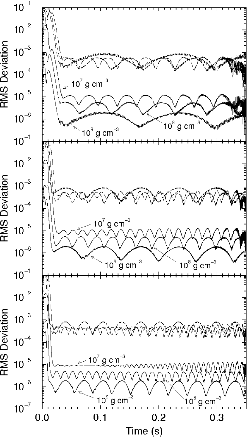
Figure 2.— Plot of RMS deviations in pressure (solid curves) and velocity (dashed curves) for simulations of propagating model flames performed at densities of $10^{7}$ $10^{8}$, and $10^{9}\ \mathrm{g\ cm^{-3}}$ with a fixed flame speed of $6\times 10^{6}\ \mathrm{cm\ s^{-1}}$. The simulations were performed on a uniform domain with 256 zones (top panel), 512 zones (middle panel), and 1024 (bottom panel) zones.

Table 1Simulation Properties

density	${\rm c_{s}}$ (fuel)	$t_{\rm soundcrossing}$
$10^{9}\ \mathrm{g\ cm^{-3}}$	$10^{8}\ \mathrm{cm\ s^{-1}}$	$10^{-3}{\mathrm{s}}$
2	9.04	4.42
1	8.06	4.96
0.5	7.17	5.58
0.3	6.58	6.08
0.1	5.50	7.27
0.05	4.82	8.30
0.03	4.40	9.09
0.01	3.59	11.1

3.2. Sources of acoustic noise

The simulations performed for this study indicate that there are two principal sources of noise, transient noise resulting from the initial conditions and steady rhythmic noise produced as the model flame propagates across the simulation domain. We observed noise from these sources in the simulation results in three forms, described below, one from the initial transient and two from the propagation noise. Though not shown here in detail, by comparing these metrics for the multistage flame to a single-stage flame with comparable static energy release, we confirmed that the multistage scheme adds no significant noise.

The most obvious feature of the simulations is a large amount of noise early in the simulations. This may be observed in all of the RMS deviation figures as the large deviations on the left-hand side (early time region) of the plots. This transient results from the method of initiating the burning. The burned region is created by setting $Y_{{\rm ion},f},$ and $\bar{q}_{f}$ to the appropriate values for the given density and fuel composition and the profile of the flame to

$$\phi_{1}(x)=\frac{1}{2}\left[1.0-\mathrm{tanh}\left[(x-x_{0})/L\right]\right]$$ (23)

where $L=b\Delta x/2$ (Vladimirova et al., 2006), $\phi_{2}=\phi_{1}$, $\phi_{3}=0$, and here $x_{0}$ is the initial position of the flame front, 5% of the distance across the domain. This prescription produces initial conditions that depart slightly from the relaxed result obtained after some evolution, and the relaxation occurring during the initial evolution produces the large amounts of noise observed early on. The perturbation in this case is a large sound pulse that propagates across the domain.

Observation of the RMS deviation curves for a particular density in Figure 2 indicates that the duration of the transient noise depends on resolution of the simulation. This occurs because the width of the thickened flame is set by the resolution of the simulation grid, and the duration of this pulse is set by the flame self-crossing time. The wider flames at lower resolutions produce an initial transient sound wave that has the correspondingly longer wavelength thereby taking the correspondingly longer time to all propagate out of the domain. As an example we consider simulations of Figure 1, performed with $\rho=10^{9}\ \mathrm{g\ cm^{-3}}$ and $s=3.89\times 10^{6}$ cm s^-1. The observed times for the transient pulse to pass completely across the grid were 0.016, 0.026, and 0.047 s for resolutions of 1024, 512, and 256 zones, respectively. These times were measured by observing the pressure wave propagate across the simulation domain and agree well with the duration of the transients observed in the deviations. The times are very consistent with the flame self-crossing time, $4\Delta x/s$, which is also the time for the flame profile to come into equilibrium, and therefore for the burning rate to stabilize. Thus the duration in number of time steps, $4\Delta x/s/(0.8\Delta x/c_{s})\approx 1000$, is similar for all three resolutions, as seen in Figure 1.

As the flame profile moves across the regular underlying grid, the slight changes in the profile due to the spatial quantization lead to a small, rhythmic variation of the burning rate. This produces a pressure wave train propagating out through the fuel with a specific form characterized by the quantization and with a period determined by time for the flame profile to shift by one zone. This leads to the high frequency oscillations readily observed in Figure 1 after the initial transient. In Figure 2 this noise may be seen as the small high-frequency (period $<0.005$ s) features on the curves and is most obvious in the $\rho=10^{9}\ \mathrm{g\ cm^{-3}}$ curves of the 256 zone simulation (top panel). As an example, we consider the simulation at $\rho=10^{9}\ \mathrm{g\ cm^{-3}}$ with a flame speed of $s=3.89\times 10^{6}\ \mathrm{cm\ s^{-1}}$ at our highest resolution, shown in Figure 1. The wave propagating through the fuel has an average wavelength of $6.76\times 10^{5}\ \mathrm{cm}$, which with a sound speed of $8\times 10^{8}\ \mathrm{cm\ s^{-1}}$ gives a period of $8.45\times 10^{-4}$ s. The flame front propagates through 16 computational zones in an average of 0.0135 s, giving $8.43\times 10^{-4}$s to burn each zone. With the fuel at rest, the flame front should move within the computational domain at $s\rho_{\rm fuel}/\rho_{\rm ash}$ (this is higher than the flame speed due to expansion), which gives a zone crossing time of $8.37\times 10^{-4}$ s, using the expansion for this density from Calder et al. (2007). All these checks prove completely consistent.

The regular oscillating pattern (with period 0.1 s and larger) of the noise visible in Figure 2 originates from the variation in size of the region of the emitted wave train over which the deviation is being averaged. From the discussion above this wave train has a wavelength given by equating the sound crossing time of the disturbance with the time for the flame to cross a single zone, $\lambda/c_{s}=\Delta x/v_{f}$. Since the sound field is otherwise essentially flat, averaging over an integer number of these wavelengths will give about the same result. Thus we expect a regular pattern in the noise measured at a period determined by the time for the averaging interval to shrink by one wavelength. The interval is shrinking at the same speed that the flame is moving across the computational domain, given above, and dividing the wavelength of the emitted train by this gives a period of $P=\lambda/v_{f}=c_{s}\Delta x/(s\rho_{\rm fuel}/\rho_{\rm ash})^{2}$. This relation reproduces the linear dependence on resolution seen in the results, and shows that the dependence on density enters through both the sound speed and the expansion factor. We have confirmed that this relation reproduces the periods in the figures, e.g. $P=0.24$ s for $s=6\times 10^{6}\ \mathrm{cm\ s^{-1}}$, $\rho=10^{9}\ \mathrm{g\ cm^{-3}}$ and our coarsest resolution. This result represents two bumps in the noise figures because we are taking the RMS deviation, losing the sign.

Finally, we note that as the flames approached the edge of the simulation domain and most of the fuel on the domain had burned, the magnitude of both the high frequency oscillations and the regular pattern in the deviation increased (as may be observed on the right hand side of the curves, especially at the lowest density, $10^{7}\ \mathrm{g\ cm^{-3}}$). This increase occurs because what little fuel remains samples the region very near the flame, which is expected to have the most noise.

4. The progression of a flame from single-point initiation

It is useful to describe with some detail the progress of events involved in the GCD mechanism, and how our simulation setup captures these events. In the centuries before the Ia event, when the WD has accreted enough matter to ignite carbon burning in the center, there is an expanding convective carbon-burning core (see e.g. Woosley et al. 2004). This state is already a runaway, because the temperature at the center will continue to monotonically rise. Ignition occurs during this convective phase when the local heating time $\tau_{\rm heat}\simeq c_{P}T/\epsilon_{\rm nuc}$, where $c_{P}$ is the specific heat at constant pressure and $\epsilon_{\rm nuc}$ is the nuclear energy deposition rate, becomes shorter than the eddy turnover time $\tau_{\rm edd}\simeq 10$-100 seconds. At this point the burning runs away locally, the $\mathrm{{}^{12}C}$ and $\mathrm{{}^{16}O}$ fuel converts entirely to Fe-peak elements and a flamelet is born.

While the rate of formation of ignition points is unclear, it is believed that ignition of local flamelets in the core of the WD is a fairly stochastic process (Woosley et al., 2004; Wunsch & Woosley, 2004). For this study we will work under the hypothesis that the ignition conditions are rare at the time the ignition occurs. This means that the ignition grows from a small ($\lesssim$ 1 km) region somewhere in the first temperature scale height ($\sim 400$ km) near the center of the star, and the second ignition is long enough after this ($\gtrsim 1$ sec) to be unimportant (see Woosley et al. 2004 for a discussion of how these scales arise.) This picture is representative of the ignition conditions found by Höflich & Stein (2002) in their study of the pre-runaway phase, but is somewhat in contrast to the conclusions of some of the above work (e.g. Woosley et al., 2004), and is essentially the opposite hypothesis to that taken by Röpke et al. (2006a). Single-point ignition is plausible within the current uncertainties and is quite useful for our purpose here of understanding the dynamics of a flame bubble and characterizing our numerical methods.

4.1. General Simulation Setup

In order to simplify our study of single-bubble dynamics we begin our simulation with no velocity field in the stellar core. This is, in fact, a poor approximation to reality because the typical outer scale velocity in the convective core is expected to be $\sim 100$ km s^-1 (Kuhlen et al., 2006), which is comparable to the laminar flame propagation speed in this part of the star (Timmes & Woosley, 1992; Chamulak et al., 2007). This means that the strongest initial source of perturbations on the flame surface, and therefore seeds of the later R-T modes, is likely to be the turbulence in the convective core flow field. The convection field is, however, not strong enough to destroy the flamelet once it is born. We feel neglection of the the convective flow field in this initial study justifiable for two reasons. First, we would like to understand the dynamics of the bubbles and flame surface near the core first without the additional complication of the turbulent flow. Second, it will be challenging to interpret the effects that a turbulent field in two dimensions subject to the imposed axisymmetry might produce. Any off-axis feature acts effectively as a ring, an effect that causes enough difficulty even with static initial conditions. Also Livne et al. (2005) find that the general outcome of off-center ignitions is not strongly effected by the presence of a convection field.

We perform two-dimensional axisymmetric simulations with the FLASH adaptive-mesh hydrodynamics code (Fryxell et al., 2000; Calder et al., 2002). We begin our simulations with at 1.38 $M_{\odot}$ WD with a uniform composition of equal parts by mass of $\mathrm{{}^{12}C}$ and $\mathrm{{}^{16}O}$. This model has a central density of $2.2\times 10^{9}$ g cm^-3, a uniform temperature of $4\times 10^{7}$ K, and a radius of approximately 2,000 km. A spherical region on the symmetry axis is converted to burned material with $\phi_{1}$ given by eq. (23) with $x=|\vec{r}-\vec{r}_{\rm off}|$ and $x_{0}=r_{\rm bub}$, $\phi_{2}=\phi_{1}$, and $\phi_{3}=0$, where $\vec{r}_{\rm off}$ is the location of the center of the ignition point. The density is chosen to maintain pressure equilibrium with the surrounding material. Thus the radius of the flame bubble, $r_{\rm bub}$, is the approximate location of the $\phi_{1}=0.5$ isosurface, and all simulations in this paper begin with a spherical bubble of radius 16 km. This is the smallest bubble that is reasonably well resolved (having $\phi_{1}$ very close to 1 at the center) at 4 km resolution, that used in the parameter study presented in section 5. The basic parameters and some results are listed in Table 2, and will be discussed below.

Our adaptive mesh refinement has been chosen to capture the relevant physical features of the burning and flow at reasonable computational expense. We choose to refine on strong density gradients everywhere, and strong velocity gradients in the burned material. At the beginning of the simulation all of the star is resolved to 16 km resolution regardless of the maximum allowed resolution for reasons of hydrostatic stability (Plewa, 2007). In regions with $\rho<5\times 10^{5}$ g cm^-3 refinement is not requested, which includes all of the region outside the star. Regions where the flame is actively propagating ($0.1<\phi<0.9$, and non-trivial flame speed) are required to be fully refined in order to properly propagate the flame front. In the interest of limiting computational expense, the refinement is limited to a finest resolution of 32 km outside a radius of 2500 km, which is above the the surface of the star in all cases treated here. This constraint will be relaxed in future work, but the bulk kinetic motion of the surface flow is not expected to be affected by this choice.

Figure 3.— Critical wavelength for flame surface perturbations $\lambda_{c}=6\pi s^{2}/Ag$ in the initial WD.

4.2. Stages of Flamelet Evolution

The major stages in the evolution of the bubble can be roughly understood by comparing the bubble’s size to the critical wavelength for the unstable Rayleigh-Taylor growth of flame surface perturbations. We define $\lambda_{c}\equiv 6\pi s^{2}/Ag$ (Khokhlov, 1995), where $g$ is the local gravity, $s$ is the laminar flame speed, and $A=(\rho_{\rm fuel}-\rho_{\rm ash})/(\rho_{\rm fuel}+\rho_{\rm ash})$ is the Atwood number. Below $\lambda_{c}$, $s$ is high enough that perturbations in the flame surface can be “polished out” by burning, so that the surface remains laminar and simple. Above $\lambda_{c}$, R-T is strong enough that perturbations will grow instead, leading to a complex, disordered flame structure down to a scale of order $\lambda_{c}$. (See Khokhlov 1995 for an extensive discussion.) As shown in Figure 3, $\lambda_{c}$ drops quickly with radius, mainly due to the increasing gravity as one moves away from the center of the star, and after this due to the falling flame speed. We take $r_{\rm bub}<\lambda_{c}$ in all cases, so that our assumption of a spherical bubble at rest is physically justifiable (Fisher et al., 2007).

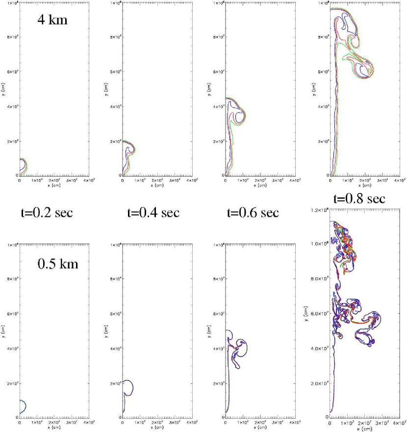
Figure 4.— Stages of bubble growth at different resolutions. The initial radius of the bubble was 16 km centered at 40 km from the center of the star, contours are shown for the progress variable $\phi=0.1$ (green), 0.5 (red), and 0.9 (blue).

Initially bubbles can be thought of as moving from lower left to upper right (growing and rising) in Figure 3 (see Zingale & Dursi 2007). We distinguish three phases of the bubble evolution and rise in terms of $\lambda_{c}$. Each of these phases can be seen in Figure 4, where we show the evolution of the flame surface with time for two different resolutions: our typical resolution, 4 km, and our highest resolution, 0.5 km. Initially, while small and near the center with $r_{\rm bub}<\lambda_{c}$, the flame bubble will grow according to the laminar flame speed, roughly keeping a spherical shape. This structure is evident at $t=0.2$ seconds, where the bubble has already grown to a radius of about 30 km, twice its original size.

Eventually as the bubble rises and grows, it will reach the point when $r_{\rm bub}\sim\lambda_{c}$. For our case this occurs at a little over 100 km radius. As seen at $t=0.4$ sec, the bubble forms a R-T roll at approximately its full dimensions, the first scale that is unstable. This feature shows some differences with resolution, but generally the same kind of feature (a roll) has appeared in both simulations. Crossing $\lambda_{c}$, the bubble is now a R-T unstable flamelet. The subsequent evolution is resolved in our simulation until $\lambda_{c}$ falls below the grid scale. Thus we will term the second stage of evolution as the resolved R-T stage. The R-T structure becomes unresolved at approximately 350 and 500 km radius for 4 and 0.5 km resolution respectively. Thus by t=0.6 seconds, the 4 km simulation has already entered the unresolved regime, while the 0.5 km simulation has nearly entered it. This is evidenced by the separation between consecutive contours in the progress variable caused by strong advection of material within the flame front.

The rest of the bubble rise and burn is dominated by unresolved R-T burning. The bubble continues to grow, both due to burning and expansion of the material under decreasing pressure. Its top generally reaches the surface at approximately 1.0 seconds (“breakout”), after which it mostly exits the interior of the star and expands strongly to create the flow around the stellar surface. A notable difference between our evolution and that seen by (Röpke et al., 2006b) is the presence of the “stem” below the rising bubble. This stem is absent in non-reactive rising bubbles (Vladimirova, 2007), but it is mysterious that it is completely absent in the level-set reactive flow simulations. This might be related to the fact that the initial bubbles used by Röpke et al. (2006b) are too large and far off-center to capture either the laminar or resolved R-T evolution stages, but more investigation is necessary. Though both simulations in Figure 4 are unresolved at $t=0.8$ seconds, comparing the two provides a good demonstration of the enhancement in flame surface facilitated by smaller scale structure.

As mentioned in section 2, any flame tracking method that depends on the advection of a scalar field faces difficulties in the highly turbulent flow produced in the unresolved R-T stage. Measures must be taken to compensate for the finite resolution of the simulation, otherwise the flame ceases to propagate correctly because the turbulence destroys the necessary structure for self-propagation of the scalar field. This problem is particularly relevant to the simulation of WD deflagrations, as has been extensively discussed by previous authors (Khokhlov, 1995; Gamezo et al., 2003; Schmidt et al., 2006). R-T can create turbulence down to the scale $\lambda_{c}$, below which the flame is able to polish out the mixing perturbations. It is thought (Khokhlov, 1995) that the details of this small-scale behavior need not be followed explicitly. If the overall dynamics of the flame surface are determined by the large scale perturbations, simulations of moderate resolution (which may however be only just possible today in 3-d) can determine the evolution of the burning front. This is called self-regulation, and the open question is: What resolution is “enough”? This is currently under debate, and we will argue here that we have enough resolution for some purposes and can make statements about others based on trends that we see with resolution.

Schmidt et al. (2006) attempted to compensate for the shortcoming of the limited resolution by artificially enhancing the propagation speed of the flame front based on a measure of local turbulence. Such complex measures should not be necessary if self-regulation holds, thus we have taken what we consider to be a conservative approach, making the smallest possible adjustment to the front propagation speed and evaluating the inaccuracy directly via resolution study. We enforce a minimum flame speed (which therefore acts effectively as an enhancement) that is intended to ensure $\tau_{\rm R-T}\gtrsim\tau_{\rm flame}$ where, for flame width $\delta$, $\tau_{\rm R-T}\approx\sqrt{\delta/Ag}$ is the characteristic R-T rise time and $\tau_{\rm flame}\approx\delta/s$ is the flame self-crossing time. Since our flame width is proportional to the resolution, this leads to a limit $s\geq\alpha\sqrt{Agm_{f}\Delta x}$, where $\Delta x$ is the resolution, $\alpha$ is a geometrical factor that is different in two and three dimensions, and $m_{f}$ is a calibrated constant.

We have determined $m_{f}$, the constant that determines when the flame model “breaks”, empirically by running two-dimensional flame-in-a-box simulations like those of Khokhlov (1995) and Zhang et al. (2007). We evaluated the range of $s$ over which self-regulation holds, in which the burning rate, $\dot{m}_{\rm burned}=\rho L^{(d-1)}s_{\rm eff}$ is determined by the box size, $L$, such that $s_{\rm eff}=\alpha\sqrt{AgL}$, independent of $s$. In two dimensions $\alpha=0.28$ and in three dimensions, as found by previous authors, $\alpha=0.5$. We found that the self-regulated regime is bounded above by $s\simeq\sqrt{AgL}$, corresponding to the requirement $\lambda_{c}\lesssim L$, and below by $s\simeq\alpha\sqrt{Ag0.04\Delta x}$. In our WD simulations we have used the value for $\alpha$ from three-dimensional simulations, although we are working in two-dimensional cylindrical geometry, and $m_{f}=0.04$. These values have been confirmed by preliminary three-dimensional flame-in-a-box calculations, which will be discussed in a separate work. Using this type of floor on $s$ requires that we explicitly turn off the flame at low density. This is done smoothly between $\rho=10^{7}\ \mathrm{g\ cm^{-3}}$ and $5\times 10^{6}\ \mathrm{g\ cm^{-3}}$, so that $s=0$ for densities below this.

4.3. Resolution Study

Some properties of the off-center deflagration model that we are trying to deduce from our simulations show dependence on the simulation resolution, while others do not. We would like to make statements as much as possible based on features that are not influenced by resolution, and where we cannot avoid it, account for the dependence in other conclusions that we draw. Problems with resolution-dependence is not entirely unexpected, since, as just discussed, a significant amount of our simulation is a priori known to be unresolved. In summary, we find that the conditions at the possible detonation point are fairly insensitive to resolution, for the resolutions considered, but that the state of the interior of the star at a given time during the runaway may only be calculated by higher resolution simulations than the 4 km at which our parameter study was performed.

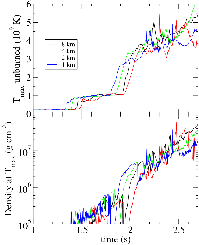
Figure 5.— Maximum temperature $T_{\rm max}$ in the lower hemisphere and the density at the same point. Shown are results from simulations where the deflagration is ignited by a bubble of flame with a radius of 16km placed 40 km off-center and for which the resolution is varied to 8, 4, 2, and 1 km. Material flowing over the surface enters the lower hemisphere at approximately 1.5 seconds and the collision occurs at approximately 2.0 seconds, at which point the material near the collision region begins to compress. We find that the conditions at the ignition point are insensitive to the simulation resolution.

Of foremost interest is the robustness of the gravitationally confined detonation (GCD) mechanism, particularly the properties in the collision and compression regions opposite the eruption point. We have performed two-dimensional simulations of various resolutions that begin from a 16 km radius burned region offset from the center by 40 km. The history of the maximum temperature, $T_{\rm max}$, in the lower hemisphere ($\theta>\pi/2$), and the density at that same point is shown in Figure 5. After the bubble has reached the surface, material – burned and unburned – begins to flow over the surface of the star towards the opposite pole. This material enters the lower hemisphere approximately 1.5 seconds after the ignition. Some of the low-density material is being shocked as it interacts with the stellar surface as it is moving around the star, giving a temperature near $10^{9}$ K. The collision of material at the lower pole occurs at approximately 2 seconds and the density of the hottest region steadily increases thereafter until the expected ignition of the detonation at $T>3\times 10^{9}$ K and $\rho>10^{7}\ \mathrm{g\ cm^{-3}}$. See section 5 for a more extensive discussion of the fluid motions in the simulation. We find that the temperature and density reached at the possible ignition point of the detonation are insensitive to the simulation resolution. This gives confidence in the robustness of the GCD scenario as a whole, in that the bulk motion of the surface flow seems to be insensitive to resolution. Sensitivity to initial conditions and assumed symmetry have not been addressed here, and will be the subject of future work.

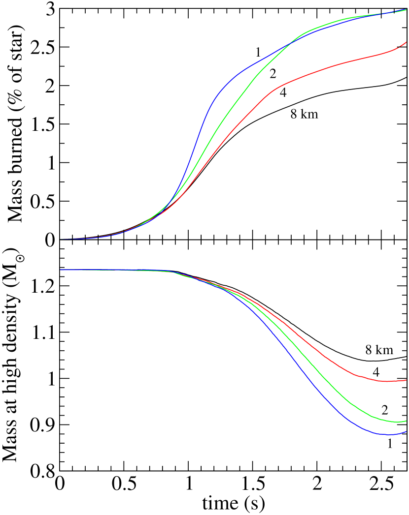
Figure 6.— Burned mass (as a fraction of the star) and stellar mass with $\rho>5.5\times 10^{7}$ g cm^-3 for simulations shown in figure 5. There is a clear dependence on resolution, with finer resolutions generally leading to more rapid evolution.

The overall amount of material burned, and therefore the amount of energy added to the star, is important for determination of the interior state (notably density) when the detonation wave sweeps through. This will set the amount and distribution of $\mathrm{{}^{56}Ni}$ and intermediate mass elements, and is therefore extremely important for the predictive power of our simulations. Shown in Figure 6 is the amount of mass burned by the rising flame and the mass of the star, which has $\rho>5.5\times 10^{7}$ (see next section). As seen in Figure 4, it appears that the bubble rises somewhat faster at higher resolutions, possibly due to the decreased numerical viscosity or to faster burning during the resolved R-T stage. Both the total burned mass and the amount of high density material show significant dependence on resolution, but it appears that convergence in the overall quantities may be just within reach. The total burned mass at 2 km and 1 km resolution is quite consistent by the time the detonation might occur, and the difference between the amount of high density material is also fairly modest considering the factor of 2 difference in resolution and the expected offset in time due to the lower numerical viscosity.

But not all the news is good. Performing a full suite of simulations at 1 km was not undertaken for this study and will be prohibitive in three dimensions, but knowing how far away convergence is lends great interpretive power to our lower resolution simulations. There is also a caution to be raised. Figure 6 does not include results at 0.5 km, although the beginning of the curve is obviously available, because much more mass is burned in this case. This occurs because while the dominant trailing vortices follow the main bubble out of the star at all lower resolutions, at 0.5 km the branch feature visible in Figure 4 at a radius of 600 km does not. This piece of flame, which has now become a ring due to the axisymmetry, stays at high density and continues to burn a significant portion of the star. It is unfortunately not possible for us to judge whether this is realistic or largely an artifact of the very different nature of vorticity conservation in two dimensions. We do note that simulations with a smaller bubble (2 km) and slightly larger offset (60 km) do not show this anomaly, and initially proceed much as those at lower resolution. This effect deserves close scrutiny as more simulations are performed, especially in 3-d. Also the shed vortices would likely not have an adverse impact if we were simulating a centrally ignited deflagration that consumed most of the WD on the way to the surface.

Table 2Properties at Detonation Ignition

$r_{\rm bub}$	$r_{\rm off}$	resolution	$t_{\rm det}$	$M_{\rm burn}$	mass at high density	max density	energy release
(km)	(km)	(km)	(s)	(% of star)	($M_{\odot}$)	($10^{8}\ \mathrm{g\ cm^{-3}}$)	($10^{50}$ erg)
Resolution Study
16	40	8	2.35	1.97	1.04	7.6	0.329
16	40	4	2.31	2.33	1.01	6.6	0.388
16	40	2	2.37	2.90	0.926	5.0	0.478
16	40	1	2.35	2.88	0.892	4.5	0.517
Offset Study
16	100	4	2.02	1.13	1.13	12	0.193
16	80	4	2.05	1.36	1.12	11	0.226
16	50	4	2.19	2.07	1.05	8.0	0.347
16	40	4	2.31	2.33	1.01	6.6	0.388
16	20	4	2.70	6.57	0.473	1.6	1.15

Note. — All values are evaluated at the time indicated, $t_{\rm det}$.

5. The distributions of outcomes prior to possible detonation

The uncertainty in the location of the initial flamelet, discussed in section 4, leads us to consider ignition of a flame bubble at several offsets, $r_{\rm off}$, from the center of the star. We find that both the time at which the detonation conditions are reached at the point opposite bubble eruption and the expansion of the star up to this time are correlated with $r_{\rm off}$. Since the expansion of the star is directly related to the density of the material through which the detonation will propagate, the observed result will be a variation in the $\mathrm{{}^{56}Ni}$ mass ejected, and that of intermediate elements.

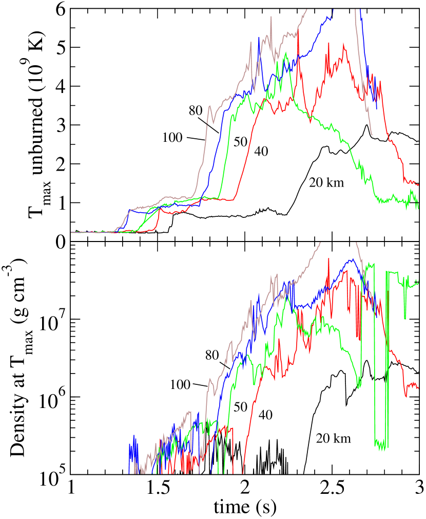
Figure 7.— Maximum temperature $T_{\rm max}$ in the lower hemisphere and the density at the same point. Shown are results from simulations at 4 km resolution with an ignited bubble of 16 km radius placed at several offsets from the center of the star, 20, 40, 50, 80, and 100 km. Material flowing over the surface enters the lower hemisphere at approximately 1.5 seconds and the collision occurs at approximately 2.0 seconds, varying some with offset, at which point the material near the collision point begins to compress.

The maximum temperature, $T_{\rm max}$, in the lower hemisphere and the density at the same point are shown in Figure 7 for a range of offsets from 20 to 100 km. The rise in temperature near $t=1.5$ seconds is when the material flowing over the surface of the star passes the equator. Collision of the surface flow at the lower pole occurs at a variety of times between 1.7 and 2.4 seconds, where $T_{\rm max}$ rises to several $10^{9}$ K, and the density steadily increases. Conservative detonation conditions require $T\gtrsim 3\times 10^{9}$ K and $\rho\gtrsim 10^{7}$ g cm^-3 (Röpke et al., 2006b; Niemeyer & Woosley, 1997). These are met at 2.02, 2.05, 2.19 and 2.31 seconds for 100, 80, 50 and 40 km respectively. Several other properties of the star at the time when the ignition is expected to occur are listed in Table 2, particularly the total energy released up to that point, in addition to the total burned mass. Note that the total binding energy is $4.95\times 10^{51}$ erg, so that none of cases here come close to unbinding the star; that is expected to occur during the detonation phase. Having only flame burning, our models continue after the detonation point and show that the detonation conditions appear to be robust and long-lived, especially at the larger offsets. Our 20 km simulation expands the star much more by the time of the collision, due to more burning occurring in the interior, and may not reach conditions sufficient for detonation. This certainly indicates that the GCD mechanism is likely to fail for ignition points very close to the center.

Figure 8.— Radius and polar angle, $\theta$, location of $T_{\rm max}$ point for simulation with $r_{\rm bub}=16$ km and $r_{\rm off}=40$ km. The region above the surface ($r\simeq 2\times 10^{8}\ \mathrm{cm}$) is heated as material collides. Material pushed toward the star from the collision point then interacts with the stellar surface to form a hot, dense region that penetrates into the outer layers of the star.

The radius and the polar angle ($\theta$) of the maximum temperature point are shown in Figure 8, demonstrating the evolution of conditions that lead to the detonation ignition. The initial surface of the star is at $r=2\times 10^{8}$ cm. Thus we see that the temperature maximum moves around the surface between 1.5 and 2.0 seconds, then shifts to the pole at the collision. Note that this jump is not material motion. At approximately 2.2 seconds, material confined between the collision point and the star becomes the hottest, and the hot spot moves steadily inward from $2\times 10^{8}$ cm. During this time the hot spot is not always precisely on the axis. Eventually the compression subsides and this hot spot dissipates. While the hot spot moves into the star with a speed of approximately $10^{8}$ cm s^-1, material ahead of it (closer to the star) is nearly at rest, and that behind it is moving in at just above $10^{9}$ cm s^-1, so that the hot spot occurs in the accumulation.

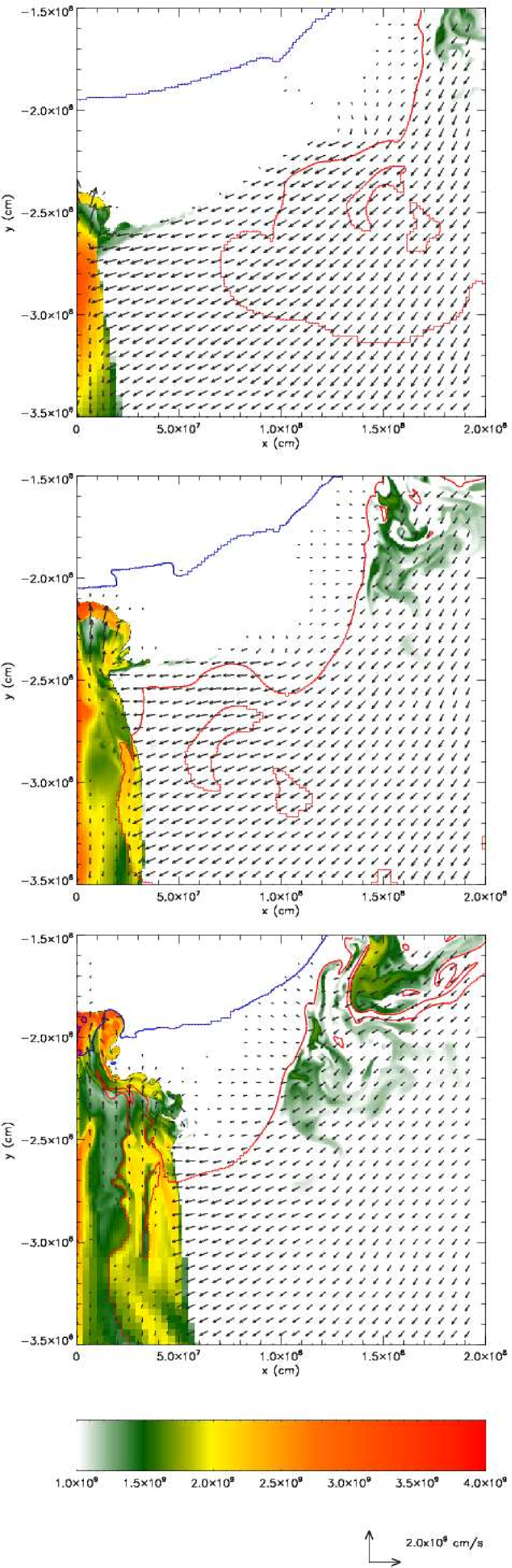
Figure 9.— Detail of flow near the collision and detonation region for the $r_{\rm off}=40$ km case, from top to bottom at $t=2.07$, 2.19, and 2.32 seconds. Temperature is shown in color and contours are shown at $\rho=10^{7}$ g cm^-3 (blue) and at the edge of the burned material ($\phi=0.1$, red). Velocity vectors smaller that $10^{8}$ cm s^-1 are not shown. A stagnation point is formed above the surface of the star from which material is projected out along the axis and compressed against the surface of the star, where the detonation is expected to occur.

A detailed view of the flow near the collision region is shown in Figure 9, where we see that a stagnation point is formed in the colliding unburned material. From this, material is projected out along the axis and toward the stellar surface, compressing the surface layers of the star toward ignition conditions. The phrase “gravitational confinement” does not convey the full impression of what is occurring. The detonating material appears to be inertially confined by flow originating at the collision point, although the amount of compression occurring likely reflects both the strongly gravitationally stratified WD surface and a certain amount of assistance from gravity, such that both high gravity and and a flow with significant inertia are required to reach such high temperatures and densities. The collision itself arises because the material is gravitationally bound, however, it is the kinetic motion imparted to the material by the expanded bubble at the breakout point that eventually leads to the (gravitationally assisted) confinement.

In the GCD scenario, because so little material is burned during the deflagration phase, the amount of $\mathrm{{}^{56}Ni}$ produced in the supernova is determined by the density distribution during the detonation phase. In lieu of simulating the propagation of the detonation, which will be performed in future work, we have measured the mass of material above $5.5\times 10^{7}$ g cm^-3. This limit is obtained from the density at which material in the W7 model (Nomoto et al., 1984) burned to only 50% $\mathrm{{}^{56}Ni}$. This is obviously only a rough estimate, but is good enough for measuring the trend with offset distance that we are interested in here. The bottom panel of Figure 10 shows how this possible $\mathrm{{}^{56}Ni}$ mass decreases as the star expands during the deflagration phase. The curves are marked at the expected launch time of the detonation, where the temperature and density first exceed $3\times 10^{9}$ K and $10^{7}$ g cm^-3 together.

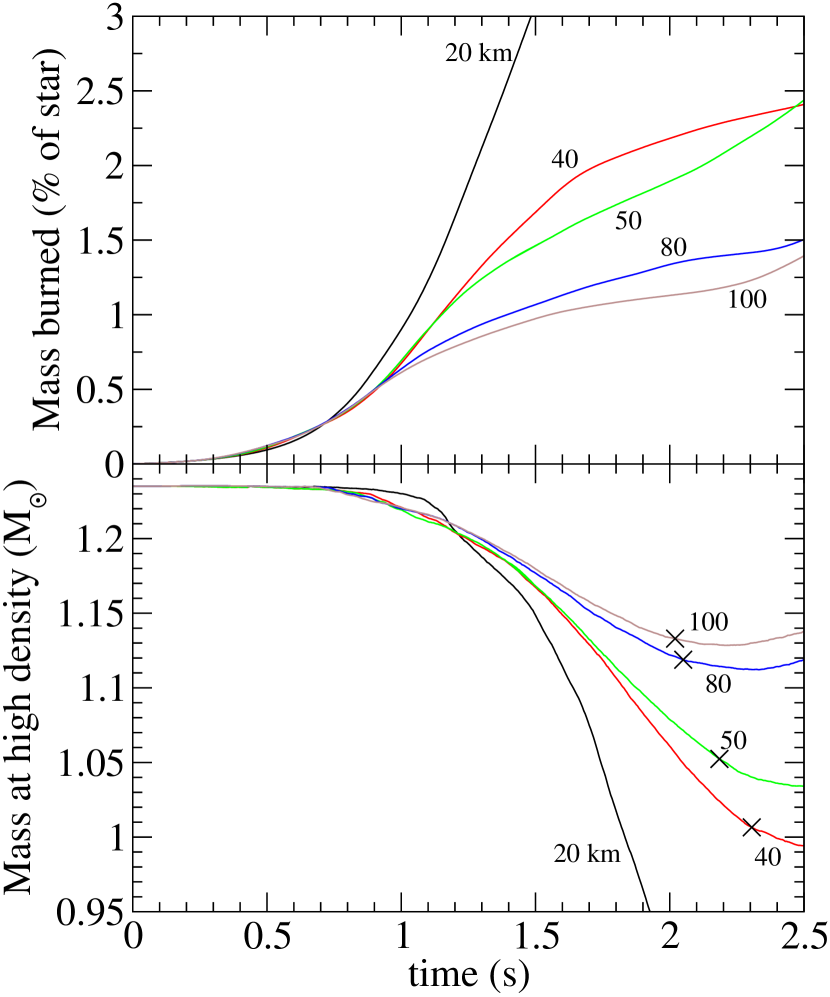
Figure 10.— Burned mass (as a fraction of the star) and stellar mass with $\rho>5.5\times 10^{7}$ g cm^-3 for same simulations as in Figure 7. The time at which a detonation is expected to be launched is marked with a $\times$ for each case. Larger offsets are expected to produce more $\mathrm{{}^{56}Ni}$ in the ejected material.

We find that the amount of $\mathrm{{}^{56}Ni}$ expected in the ejecta is correlated with the offset of the initial (small) ignition region. Larger offsets can produce more $\mathrm{{}^{56}Ni}$ for two reasons: (1) less energy is released in the deflagration phase, and therefore the star has expanded less when the detonation occurs, and (2) the detonation conditions happen sooner so that the star has had less time to expand. It does appear that the first of these is the dominant effect. The top panel of Figure 10 shows the mass burned as a fraction of the star with time. Larger offsets burn less of the star during the bubble rise and breakout, leading to less expansion of the star.

The $\mathrm{{}^{56}Ni}$ mass estimates we have found here are fairly high, but as seen in section 4.3 this resolution (4 km) appears to somewhat underestimate the burned mass and overestimate the possible $\mathrm{{}^{56}Ni}$ at the detonation time. We are not claiming to have performed an absolute calculation of the $\mathrm{{}^{56}Ni}$ mass for a given ignition point offset; we have instead demonstrated a trend that appears to be robust with respect to the physical processes that are occurring. We hope that in the future, with higher resolution such that self-regulation of the burning is strong enough that we can constrain the R-T phase better, we may be able to construct a fully predictive model. There are, however several steps that should be taken in the mean time, including three-dimensional studies that are underway (Jordan et al., 2007), and studies of flame bubble response to the strong convection expected to be present in the WD core when the ignition occurs. The current level of calculation is, however sufficient for measuring trends such as how things might change with the relative C/O fraction in the interior of the WD.

6. Conclusions

We have shown that in the GCD picture of a delayed detonation of a WD near the Chandrasekhar mass, the properties of the WD at detonation, notable the density distribution, are systematically correlated with the offset of the ignition point of the deflagration. Assuming that the detonation phase proceeds as in previous simulations, this will cause a variation in the $\mathrm{{}^{56}Ni}$ mass ejected in the supernova. The position of the ignition point within the inner few 100 km of the WD is expected to be stochastically determined by the turbulent flow in this region. GCD thus provides a possible explanation for the variety of $\mathrm{{}^{56}Ni}$ masses seen in Type Ia Supernovae.

We find that the conditions (temperature and density reached) at the candidate launch point of the detonation are insensitive to the resolution of the simulation for resolutions studied here ($\leq 8$ km). This is a good mark for the robustness of the GCD mechanism, but more work is needed, especially related to the possibility of vortex shedding early in the bubble rise and the strong convection that should be present in the core at the time of ignition. We have indications of numerical convergence in both the total burned mass and the mass of dense material, and therefore the predicted $\mathrm{{}^{56}Ni}$ mass produced by a given ignition offset. But caution is advisable: the mass burned during the highly Rayleigh-Taylor (buoyancy-driven) unstable rise of the burned region through the star is seen to vary with resolution, generally progressing faster with higher resolution, even though convergence in the final value appears to have been reached. Also, converged results (in the extremely limited sense indicated here) appear to require 2 km or possibly 1 km resolution, which is prohibitive in three dimensions. Even here, our parameter study has been performed at 4 km resolution for efficiency. Thus we are able to predict trends in the $\mathrm{{}^{56}Ni}$ mass, but not the actual value ejected for a given offset.

Our method for following the nuclear energy release, including neutronization, with an ADR flame model was described in detail. This method reproduces the energy release and hydrodynamic characteristics of the nuclear burning by following a limited number of parameters coupled to an artificially thickened flame front. We have demonstrated that the energy release adds a minimal amount of unwanted acoustic noise (RMS velocity $<\rm few\times 10^{-4}$) to the simulation, largely removing this source of unrealistic seeds for the instabilities in the rising flame surface.

References

- Asida et al. (2007) Asida, S., Townsley, D. M., Calder, A. C., Zhiglo, A., Jena, T., Khokhlov, A., & Lamb, D. Q. 2007, ApJ, in preparation
- Calder et al. (2002) Calder, A. C., Fryxell, B., Plewa, T., Rosner, R., Dursi, L. J., Weirs, V. G., Dupont, T., Robey, H. F., Kane, J. O., Remington, B. A., Drake, R. P., Dimonte, G., Zingale, M., Timmes, F. X., Olson, K., Ricker, P., MacNeice, P., & Tufo, H. M. 2002, ApJS, 143, 201
- Calder et al. (2004) Calder, A. C., Plewa, T., Vladimirova, N., Lamb, D. Q., & Truran, J. W. 2004, ArXiv Astrophysics e-prints, astro-ph/0405162
- Calder et al. (2007) Calder, A. C., Townsley, D. M., Seitenzahl, I. R., Peng, F., Messer, O. E. B., Vladimirova, N., Brown, E. F., Truran, J. W., & Lamb, D. Q. 2007, ApJ, 656, 313
- Chamulak et al. (2007) Chamulak, D. A., Brown, E. F., & Timmes, F. X. 2007, ApJ, 655, L93
- Fisher et al. (2007) Fisher, R. T., Vladimirova, N., Jordan, G. C., & Lamb, D. Q. 2007, ApJ, in preparation
- Fryxell et al. (2000) Fryxell, B., Olson, K., Ricker, P., Timmes, F. X., Zingale, M., Lamb, D. Q., MacNeice, P., Rosner, R., Truran, J. W., & Tufo, H. 2000, ApJS, 131, 273
- Gamezo et al. (2004) Gamezo, V. N., Khokhlov, A. M., & Oran, E. S. 2004, Physical Review Letters, 92, 211102
- Gamezo et al. (2005) —. 2005, ApJ, 623, 337
- Gamezo et al. (2003) Gamezo, V. N., Khokhlov, A. M., Oran, E. S., Chtchelkanova, A. Y., & Rosenberg, R. O. 2003, Science, 299, 77
- Höflich & Stein (2002) Höflich, P. & Stein, J. 2002, ApJ, 568, 779
- Hillebrandt & Niemeyer (2000) Hillebrandt, W. & Niemeyer, J. C. 2000, ARA&A, 38, 191
- Jordan et al. (2007) Jordan, G. C., Fisher, R., Townsley, D. M., Calder, A. C., Asida, S., Graziani, C., Lamb, D. Q., & Truran, J. W. 2007, ApJ, submitted
- Khokhlov (1983) Khokhlov, A. M. 1983, Soviet Astronomy Letters, 9, 160
- Khokhlov (1991) —. 1991, A&A, 245, 114
- Khokhlov (1995) —. 1995, ApJ, 449, 695
- Khokhlov (2000) —. 2000, ArXiv Astrophysics e-prints, astro-ph/0008463
- Kuhlen et al. (2006) Kuhlen, M., Woosley, S. E., & Glatzmaier, G. A. 2006, ApJ, 640, 407
- Langanke & Martínez-Pinedo (2000) Langanke, K. & Martínez-Pinedo, G. 2000, Nuclear Physics A, 673, 481
- Livne et al. (2005) Livne, E., Asida, S. M., & Höflich, P. 2005, ApJ, 632, 443
- Niemeyer & Woosley (1997) Niemeyer, J. C. & Woosley, S. E. 1997, ApJ, 475, 740
- Nomoto et al. (1984) Nomoto, K., Thielemann, F.-K., & Yokoi, K. 1984, ApJ, 286, 644
- Plewa (2007) Plewa, T. 2007, ApJ, in press. (astro-ph/0611776)
- Plewa et al. (2004) Plewa, T., Calder, A. C., & Lamb, D. Q. 2004, ApJ, 612, L37
- Reinecke et al. (1999) Reinecke, M., Hillebrandt, W., Niemeyer, J. C., Klein, R., & Gröbl, A. 1999, A&A, 347, 724
- Röpke et al. (2006a) Röpke, F. K., Hillebrandt, W., Niemeyer, J. C., & Woosley, S. E. 2006a, A&A, 448, 1
- Röpke et al. (2003) Röpke, F. K., Niemeyer, J. C., & Hillebrandt, W. 2003, ApJ, 588, 952
- Röpke et al. (2006b) Röpke, F. K., Woosley, S. E., & Hillebrandt, W. 2006b, ApJ, Submitted. (astro-ph/0609088)
- Schmidt et al. (2006) Schmidt, W., Niemeyer, J. C., Hillebrandt, W., & Röpke, F. K. 2006, A&A, 450, 283
- Smiljanovski et al. (1997) Smiljanovski, V., Moser, V., & Klein, R. 1997, Combustion Theory Modelling, 1, 183
- Timmes & Swesty (2000) Timmes, F. X. & Swesty, F. D. 2000, ApJS, 126, 501
- Timmes & Woosley (1992) Timmes, F. X. & Woosley, S. E. 1992, ApJ, 396, 649
- Vladimirova (2007) Vladimirova, N. 2007, Comb. Theory and modelling, 11, 377
- Vladimirova et al. (2006) Vladimirova, N., Weirs, G., & Ryzhik, L. 2006, Combust. Theory Modelling, 10, 727
- Woosley et al. (2004) Woosley, S. E., Wunsch, S., & Kuhlen, M. 2004, ApJ, 607, 921
- Wunsch & Woosley (2004) Wunsch, S. & Woosley, S. E. 2004, ApJ, 616, 1102
- Xin (2000) Xin, J. 2000, SIAM Review, 42, 161
- Zhang et al. (2007) Zhang, J., Messer, O. E. B., Khokhlov, A. M., & Plewa, T. 2007, ApJ, 656, 347
- Zingale & Dursi (2007) Zingale, M. & Dursi, L. J. 2007, ApJ, 656, 333