Influence of Hydrodynamic Interactions on Mechanical Unfolding of Proteins

Abstract

We incorporate hydrodynamic interactions in a structure-based model of ubiquitin and demonstrate that the hydrodynamic coupling may reduce the peak force when stretching the protein at constant speed, especially at larger speeds. Hydrodynamic interactions are also shown to facilitate unfolding at constant force and inhibit stretching by fluid flows.

I Introduction

It has been widely recognized that the water environment affects the energy landscape and functionality of biomolecules in a profound way. There is, however, another solvent-related effect that is considered less frequently: the hydrodynamic interactions (HI) between individual segments of a biomolecule that moves. These interactions may affect the dynamics of conformational changes because any motion of one segment generates a local fluid flow which influences another segment.

The presence of HI is known to affects dynamic properties of soft mater. For instance, HI modify the values of diffusion coefficients in colloidal suspensions Dhont , affect the characteristics of the coil-stretch transition in polymers Larson , change the kinetic pathways of phase separation in binary mixtures Tanaka , and alter the kinetics of macromolecule adsorption on surfaces Wojtaszczyk . Much less is known about the role of HI in protein folding and unfolding processes. Dickinson Dickinson and Tanaka Tanaka2 speculated that HI might affect the kinetics of protein folding, but the actual numerical assessment of the role of HI has come with the paper by Baumketner and Hiwatari Baumketner . They have considered coarse grained models and found that HI delay folding of a $\beta$ hairpin but do not affect folding of the $\alpha$-helix.

In this paper, we consider mechanical stretching of proteins and study the relevance of HI to the process. The stretching can be accomplished in several ways and we discuss three modes: at constant speed, at constant force, and through fluid flow. We chose ubiquitin as a model system, since there is a large body of experimental Vazquez ; Chyan ; FernandezLi ; Schlierf and theoretical Makarov ; Makarov2 ; Irback ; cieplakmarszalek ; cs1 ; West data on its unfolding. A coarse-grained, Go-type model Goabe of a protein is used, constructed based on the knowledge of its native state. The Go models have been shown to give surprisingly good agreement with both the experimental results ciepho ; cieplakmarszalek ; sulkowska and all-atom molecular dynamic simulations West when it comes to stretching.

We outline the model in section 2, then introduce two different ways of tracking the evolution of the system: through Langevin Dynamics and Brownian Dynamics in sections 3 and 4 respectively. In the following sections we discuss results pertaining to the three modes of stretching and demonstrate that HI can take many roles: they inhibit unfolding by fluid flow, but make the constant force stretching faster. At constant speed, they reduce the peak force if the speed is sufficiently high. This HI-related reduction in force may be downplayed in the all-atom simulations of titin by Lu and Schulten Schulten which would provide part of an explanation for the excessively large forces obtained in these studies.

II The coarse-grained protein model

In our simulations, we use the coarse-grained, Go-type model of a protein. In the model, each residue is represented by a single bead centered on the position of the C^α atom. The successive beads along the backbone are tethered by harmonic potentials with a minimum at 3.8 Å. The other interactions between the residues are split into two classes: native and non-native. This determination is made by checking for native overlaps of all atoms in aminoacids when represented by enlarged van der Waals spheres as proposed in reference Tsai . The amino acids, $i$ and $j$, that do overlap in this sense are endowed with the effective Lennard-Jones potential $V_{ij}=4\epsilon\left[\left(\frac{\sigma_{ij}}{r_{ij}}\right)^{12}-\left(\frac{\sigma_{ij}}{r_{ij}}\right)^{6}\right]$. The length parameters $\sigma_{ij}$ are chosen so that the potential minima correspond, pair-by-pair, to the experimentally established native distances between the respective aminoacids. In order to prevent emergence of entanglements, the non-native contacts are endowed with a hard core repulsion described by the $r_{ij}^{-12}$ part of the Lennard-Jones potential combined with a constant shift term that makes the potential vanish smoothly at 4 Å. The specificity of a protein is contained in the length parameters $\sigma_{ij}$. The energy parameter, $\epsilon$, is taken to be uniform. We take $\epsilon/k_{B}=900K$, which correlates well with the data on titin and ubiquitin unfolding Pastore ; cieplakmarszalek . Thus the reduced temperature, $\tilde{T}=k_{B}T/\epsilon\;$ of 0.3 should be close to room temperature. All of the simulations reported here were performed at this temperature. Various simulation methods to study the dynamics of the system are outlined in the following sections.

III Langevin dynamics (LD)

In this case, the dynamics of a protein is assumed to be governed by the Langevin equation

$$m\ddot{{\bf r_{i}}}=-\gamma(\dot{{\bf r}}_{i}-{\bf u}({\bf r}_{i}))+{\bf F}^{c}_{i}+{\bf\Gamma}_{i}\;\;.$$ (1)

Here, ${\bf r_{i}}$ is the position of the $i$’th aminoacid, ${\bf F}^{c}_{i}$ is the net force on it due to contact potentials, $\gamma$ is the friction coefficient, and ${\bf u}({\bf r}_{i})$ denotes the solvent flow field. Finally, ${\bf\Gamma}$ is a white noise term with the dispersion obeying

$$\langle{\bf\Gamma}_{i}(t){\bf\Gamma}_{j}(t^{\prime})\rangle=2k_{B}T\gamma\delta(t-t^{\prime}){\bf I}\delta_{ij}$$

where I is the identity matrix. The white noise term mimicks the effect of the random collisions of the aminoacids with the surrounding solvent at the same time serving as a thermostat of the system. However, this scheme completely neglect the effects of HI which may exist in a real system, when the motion of one particle induces the flow influencing the dynamics of all the other particles.

In the simulations, the friction coefficient $\gamma$ is taken to be equal to $2m/\tau$ where $\tau=\sqrt{m\sigma^{2}/\epsilon}\approx 3ps$ is the characteristic time scale of oscillations in the Lennard-Jones well. The parameter $\sigma$=5 Å used in the above definition is a characteristic value of $\sigma_{ij}$ in the system. The selected value of $\gamma$ corresponds to a situation in which the inertial effects are small veit ; Hoang but the damping action is not yet as strong as in water. The equations of motion are solved by a fifth order predictor-corrector scheme.

Let us note, however, that although Langevin dynamics is commonly used in simulations of biological systems, the validity of this approach is not always well-established. Namely, as already noted by Lorentz Lorentz , the Langevin equation in the above form may only be used if there is a separation of time scales between the relaxation time of the particle (i.e. the bead) velocity $\tau_{v}=\frac{m}{\gamma}=\frac{2a^{2}\rho}{9\eta}$ and the viscous relaxation time of the solvent, $\tau_{\eta}=a^{2}\frac{\rho_{s}}{\eta}$, where $\rho$ is the density of the particle, $a$ its radius, and $\rho_{s}$ - the density of the solvent (see also the thorough discussion in the book by Mazo Mazo .) The ratio of those two time scales is proportional to $\rho/\rho_{s}$. Since the densities of proteins are only about 50% higher than those of the surrounding liquid Tsai , there is no separation of time scales between the relaxation of fluid variables and those of the bead and, strictly speaking, instead of Eq.(1) one should use the generalized Langevin Equation involving a memory kernel

$$m\ddot{{\bf r}_{i}}(t)=-\int_{0}^{t}dt^{\prime}\xi(t-t^{\prime})(\dot{{\bf r}}_{i}(t^{\prime})-{\bf u}({\bf r}_{i},t^{\prime}))+{\bf F}^{c}_{i}(t)+{\bf\Gamma}_{i}(t)\;\;.$$ (2)

where the noise is again Gaussian and related to the dissipative term through the generalized fluctuation-dissipation relation

$$\langle{\bf\Gamma}_{i}(t){\bf\Gamma}_{j}(t^{\prime})\rangle=k_{B}T\xi(t-t^{\prime}){\bf I}\delta_{ij}.$$

Such an approach is naturally much harder to implement (see, however, Min ) and thus the ordinary Langevin description as in Eq.(1) is usually resorted to. In this paper, we show that in protein unfolding simulations the results of a simple Langevin Dynamics (1) are consistent with those of Brownian Dynamics (see Sec. 4). The latter is not affected by the solvent and particle inertia effects, hence the agreement between the two methods seems to imply that non-instantaneous response of the solvent to the change of particle velocity does not play any important role in the protein unfolding processes.

IV Brownian dynamics (BD)

If the momentum relaxation time scale ($\tau_{v}$) is small in comparison to the time scales characterizing the conformational evolution of the system ($\tau_{c}$), it is appropriate to describe the dynamics in terms of equilibration of the particle configurations only. The exact definition of $\tau_{c}$ is problem dependent: if the protein is stretched by the flow $U$ then $\tau_{c}=\frac{a}{U}$, if a force $F$ acts on the molecule then $\tau_{c}=\frac{a\gamma}{F}$, and if the Brownian diffusion plays the central role in particle evolution then $\tau_{c}=a^{2}/D$, (where $D$ is the diffusion constant and $a$ the radius of the bead). The algorithm for simulations of the evolution of particle positions in this time regime has been devised by Ermak and McCammon ermak . The displacement of particle $i$ in time step $\Delta t$ (in the absence of the flow) obeys

$${\bf r}_{i}-{\bf r}_{i}^{0}=\sum_{j}\bigl{(}\nabla_{j}\cdot{\bf D}_{ij}^{0}\bigr{)}\Delta t+\frac{1}{k_{B}T}\sum_{j}{\bf D}_{ij}^{o}\cdot{\bf F}^{0}_{j}\Delta t+{\bf B}_{i},$$ (3)

where the index $0$ denotes the values of respective quantities at the beginning of the time step, ${\bf F}_{j}$ is the force exerted on particle $j$ by other particles, ${\bf D}$ is the diffusion tensor and ${\bf B}$ - a random displacement given by a Gaussian distribution with an average value of zero and covariance obeying

$$<{\bf B}_{i}{\bf B}_{j}>=2{\bf D}^{0}_{ij}\Delta t.$$ (4)

It is nontrivial to generalize the above expression to incorporate the effects of a general external flow field ansell . However, in the present case, we will be interested only in the uniform flow, in which case one gets simply

$${\bf r}_{i}-{\bf r}_{i}^{o}={\bf U}\Delta t+\sum_{j}\bigl{(}\nabla_{j}\cdot{\bf D}_{ij}^{0}\bigr{)}\Delta t+\frac{1}{k_{B}T}\sum_{j}{\bf D}_{ij}^{o}\cdot{\bf F}_{j}^{0}\Delta t+{\bf B}_{i},$$ (5)

where ${\bf U}$ is the flow velocity. If the diffusion tensor is nondiagonal, there exists a coupling between the force acting on the particle $j$ and the displacement of particle $i$ (cf. Eq.3). This coupling, mediated by the solvent, is commonly referred to as the “hydrodynamic interactions”.

Note that without the HI, the diffusion tensor is simply

$${\bf D}_{ij}=\frac{k_{B}T}{\gamma}{\bf I}\delta_{ij}$$ (6)

and we recover the overdamped limit of Eq.(1). The diffusion tensor ${\bf D}$ depends in a complicated nonlinear way on the instantaneous positions of all particles in the system. For a system of spheres, exact explicit expressions for the diffusion tensor ${\bf D}_{ij}$ exist in the form of the power series in interparticle distances, which may be incorporated into the simulation scheme Kim ; Mazur ; Brady ; Felderhof ; Ladd ; Cichocki ; Brady2 . Here we adopt a pairwise, far-field approximation of ${\bf D}$ proposed by Rotne, Prager Rotne and Yamakawa Yamakawa

$${\bf D}_{ii}=\frac{k_{B}T}{\gamma}{\bf I}$$ (7)

and

$${\bf D}_{ij}=\displaystyle\frac{k_{B}T}{\gamma}\frac{3a}{4r_{ij}}\left\{\begin{array}[]{cl}\displaystyle\left[\left(1+\frac{2a^{2}}{3r_{ij}^{2}}\right){\bf I}+\left(1-\frac{2a^{2}}{r_{ij}^{2}}\right){\bf\hat{r}}_{ij}{\bf\hat{r}}_{ij}\right],&r_{ij}\geq 2a\\ \\ \displaystyle\frac{r_{ij}}{2a}\left[\left(\frac{8}{3}-\frac{3r_{ij}}{4a}\right){\bf I}+\frac{r_{ij}}{4a}{\bf\hat{r}}_{ij}{\bf\hat{r}}_{ij}\right],&r_{ij}<2a\end{array}\right.$$ (8)

where ${\bf r}_{ij}={\bf r}_{j}-{\bf r}_{i}$ and $a$ represents the hydrodynamic radius of a bead. Since the above expression is exact only in the large $r_{ij}$ limit, the radius $a$ should be taken to be significantly smaller than 1.9 Å, which is the half of the distance between the succesive beads. On the other hand, $a$ cannot be too small, since the space along the chain is densely filled with amino acids. We take $a=1.5$ Å in our simulations, which seems a reasonable starting point for a qualitative assessment of HI impact on protein unfolding. However, further studies on the impact of $a$ on the system dynamics are needed, in particular the hydrodynamic radius might need to vary along the chain, reflecting the different sizes of the residues.

In the approximation (8), the divergence of the diffusion matrix vanishes ($\nabla_{j}\cdot{\bf D}_{ij}\equiv 0$), which further simplifies the numerical scheme. However, if the full hydrodynamic interactions are included, the divergence term should be taken into account Wajnryb .

The simulation using Eq. (3) together with (7) and (8) will be referred to as Brownian Dynamics with hydrodynamic interactions (BDHI) in contrast to a simple BD with the diagonal diffusion tensor (6).

Note that the BD describes configurational evolution of the beads on time scales in which the inertia effects of the beads and solvent molecules are negligible Naegele and, therefore, time scale separation issues discussed in Section 3 are not pertinent here. This feature favours BD as a method of choice when simulating stochastically driven motion of proteins at a coarse-grained level Dickinson .

In our previous studies on ubiqutin unfolding cs1 ; cs2 , we have used LD. Here, on the other hand, we incorporate HI within the BD approach. This calls for a comparison of the three schemes (LD, BD, and BDHI) to distinguish the effects resulting from HI and those from the usage of distinct integration schemes.

V Constant velocity stretching

Fig. 1 presents the force-extension curves for the constant-velocity unfolding at different unfolding speeds. In the simulations, both termini of a protein are attached to harmonic springs with the elastic constant $k$=0.06 $\epsilon/$Ų. The other end of the N-terminus spring is fixed whereas the C-terminus spring moves at a speed $v_{p}$. We consider three values of $v_{p}$: 0.5 , 0.05 and $v_{p}=0.005$Å$/\tau$.

In the low-speed limit, all the three data sets obtained using the LD, BD and BDHI are seen to converge to a single curve. In contrast, at large unfolding speeds, the differences between the LD and BD are pronounced. However, strictly speaking, in this time regime BD has a limited validity, because of the lack of separation between the momentum relaxation time ($t_{v}=\frac{m}{\gamma}=0.5\tau$) and the characteristic time of the aminoacid movement due to the stretching $t_{pull}=\frac{a}{v_{p}}=3\tau$ (for the highest speed quoted above). In the experiments, the separation of time scales is huge. In water $\gamma\approx 6\pi\eta a\approx 3\times 10^{-9}$ g s^-1 which leads to $\tau_{v}=\frac{m}{\gamma}\approx 0.06$ ps (for the typical aminoacid mass of $m\approx 2\times 10^{-22}$ g). On the other hand, the pulling speeds are of the order of 500 nm/s which gives $\tau_{p}\approx 0.3$ ms, thus there is a five-order-of-magnitude separation in time scales. For such a case, LD and BD simulations would give exactly the same result.

The fact that the differences between the BD and BDHI trajectories disappear in the limit of small $v_{p}$ is due to the lack of impact of HI at small velocities. To conclude, in the experimentally relevant small speed limit, the effects of HI are expected to be negligible.

An inspection of Fig. 1 indicates that in the case of high stretching speeds neglecting HI results in larger peak forces. In the high speed all-atom simulations of titin in water Schulten the forces of stretching are found to be excessively large. Such all-atom molecular dynamics programs are not geared towards hydrodynamic phenomena and may incorporate HI poorly. It is possible to consider that the excessive force could be partially due to the missing HI.

VI Force clamp unfolding

In the force-clamp AFM unfolding FernandezLi ; Schlierf one applies the stretching force to the protein terminus and monitors the end-to-end distance, $L$. The experimental data and the numerical simulations cs1 ; West show that proteins unfold in a stepwise manner at a constant force. This means that a rapid unfolding transition takes place after a certain waiting time. The smaller the force, the longer the waiting time.

In our simulations, we apply the force to the $C$ terminus of the protein, whereas the N-terminus is attached to a harmonic spring of elastic constant $k$=0.06 $\epsilon/$Ų. The unfolding trajectories of ubiquitin are presented in Fig. 2 for two values of the force, $F=2.4\ \epsilon/$Å and $F=4\ \epsilon/$Å. The LD and BD methods essentially coincide for these relatively large forces (small differences between the trajectories are merely stochastic in nature). However, the inclusion of HI changes the physics considerably – the waiting times become much smaller and the duration of the unfolding transition itself decreases from $\approx 250\tau$ to about $50\tau$ at both values of the force.

The fact that the HI facilitate protein unfolding may be understood qualitatively when one realizes that an amino acid moving away from the bulk of a protein creates a flow which drags other residues with it ( see Fig. 3).

The differences between unfolding with and without HI are further highlighted by analysis of the so called unfolding scenarios Hoang , in which one plots an average time when a given contact is broken against the contact order, i.e. against the sequential distance, $|j-i|$, between the amino acids that form a native contact. Figs. 4 and 5 compare the unfolding scenarios for LD, BD and BDHI at $F=2.4\ \epsilon/$Å and $F=4\ \epsilon/$Å respectively. Remarkably, although the differences in time scales between the unfolding with and without HI are considerable, the unfolding scenarios for the smaller force are similar (Fig. 4), which shows that the unfolding pathway of a protein is not affected by the hydrodynamic effects. However, as the force is increased, both LD and BD scenarios change (Fig. 5): the $\beta$ hairpin structure now unfolds at the end instead of at the beginning of the unfolding process. In contrast, in the case of BDHI, such a switch is not observed: the scenarios for larger and smaller forces look qualitatively similar.

VII Unfolding in a uniform flow

Finally, we study the influence of HI on the characteristics of the protein unfolding in a uniform flow with a speed of $U$. Although the process has not yet been realized experimentally, the simulations lemak1 ; lemak2 ; cs2 seem to suggest that uniform flow unfolding leads to a richer set of metastable conformations than the constant force pulling. For example, when the N terminus is anchored, ubiquitin stretches in a flow through two distinct intermediate states corresponding to a partial unzipping.

A detailed analysis of the uniform flow unfolding of ubiqutin in the absence of HI, together with the snapshots of intermediate conformations for different anchorings, can be found in cs2 . In that reference, we have mistakenly reported values of the forces in wrong units. Instead of the correct unit of $\epsilon$/Å we used $\epsilon/\sigma$, where $\sigma$ was equal to 5Å.

Fig. 6 shows examples of unfolding trajectories of ubiquitin in a uniform flow for four different flow velocities, both with and without HI. We observe that unfolding of the system with HI requires a much larger flow speed than without. This can be understood qualitatively in terms of the so-called no-draining effect Rzehak : the residues hidden inside the protein are shielded from the flow and thus only a small fraction of the residues experience the full drag force of $F=-\gamma U$ (see Fig. 7). In contrast, when no HI are present, this drag force is applied to all residues cs2 .

Notably, although the time scales and velocities involved in the protein unfolding with and without HI are completely different, the metastable states are nearly identical (see Fig. 6). This feature is related to the dynamic character of HI - they do not change the potential energy of the system and, therefore, do not affect its stationary properties. In principle, however, one could imagine a situation in which, due to the differences in dynamics imposed by HI, a system chooses alternative pathways when unfolding. This is clearly not the case here which may be related to the directed character of the disturbance (flow in this case or the force in force-clamp experiment) which imposes a prefered direction of unfolding, thus greatly reducing the set of available unfolding pathways.

The similarities in unfolding pathways of ubiquitin are further confirmed by the comparison of unfolding scenarios. As an example, Fig. 8 shows the unfolding scenario for the flow $U=3.5$ Å$/\tau$ with HI compared to $U=0.55$ Å$/\tau$ without HI (the mean unfolding times are comparable in both cases). The scenarios are very close to each other, the main difference being that the HI enhance cooperativity by breaking the contacts in a more simultaneous fashion.

VIII Summary

In summary, hydrodynamic interactions seem to affect the time scales of unfolding by a constant force and by a fluid flow in opposite way but keep the set of the possible metastable states. The HI may also reduce peak forces in stretching at a constant speed, although this effect weakens with the diminishing stretching speed.

This work has been supported by the European program IP NaPa through Warsaw University of Technology.

FIGURE CAPTIONS

Fig. 1.

Force-extension curves for the ubiquitin unfolding at a constant speed obtained using Langevin Dynamics (dotted line) and Brownian Dynamics with (thick solid line) and without (thin solid line) hydrodynamic interactions. The succesive panels correspond to the pulling speeds of $v_{p}=0.5,0.05$ and $0.005\$Å$/\tau$ from top to bottom respectively.

Fig. 2.

The end-to-end distance of the model ubiquitin as a function of time during unfolding at a constant force. The thick solid, thin solid and dotted lines correspond to the BDHI, BD, and LD simulations respectively. The upper panel corresponds to the force $F=2.4\ \epsilon/$Å, and the lower one to $F=4\ \epsilon/$Å.

Fig. 3.

The dragging effect: the moving particle creates a flow patern which affects other particles by pulling them in the direction of its motion.

Fig. 4.

Unfolding scenarios of ubiquitin at constant force of $F=2.4\ \epsilon/$Å simulated with LD (the upper panel), BD (the center panel) and BDHI (the lower panel). Open circles, triangles, squares, pentagons and solid triangles and squares correspond to contacts (36-44)–(65-72), (12-17)–(23-34), [(1-7),(12-17)]–(65,72), (41-49)–(41-49), (17-27)–(51-59), (1-7)–(12-17) respectively. The crosses denote all other contacts. The segment (23-34) corresponds to a helix. The two $\beta$-strands (1-7) and ((12-17) form a hairpin. The remaining $\beta$-strands are (17-27), (41-49), and (51-59).

Fig. 5.

The same as in Fig. 3 but for $F=4\ \epsilon/$Å.

Fig. 6.

The end-to-end distance of the model ubiquitin as a function of time during unfolding by a uniform fluid flow as illustrated by several trajectories. The lower panel corresponds to the description with the hydrodynamic interactions and the upper – without. The succesive curves in the upper panel correspond to the flows of $0.25,0.3,0.4$ and $0.5\ \text{\AA}/\tau$ bottom to top respectively. In the lower panel the flow speeds are $2.5,3.5,5.0,10.0$ Å$/\tau$ In all the simulations, the N-teminus of the protein is fixed.

Fig. 7.

The shielding effect: the particles inside a cluster experience a smaller drag force than those on the surface.

Fig. 8.

The left and right panels show unfolding scenarios without the hydrodynamic interactions ($U=0.55$ Å$/\tau$) and with the hydrodynamic interactions ($U=3.5$ Å$/\tau$) respectively.

Figure 1:

Figure 2:

Figure 3:

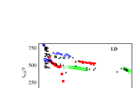
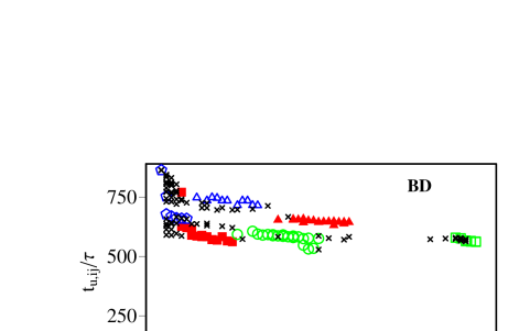
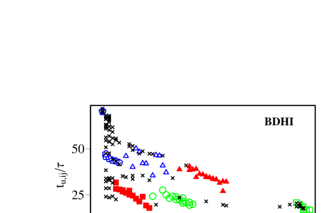
Figure 4:

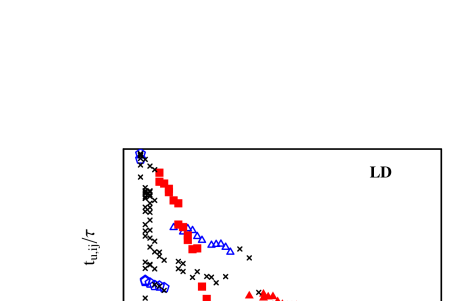
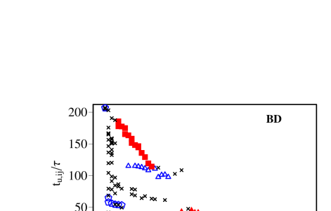
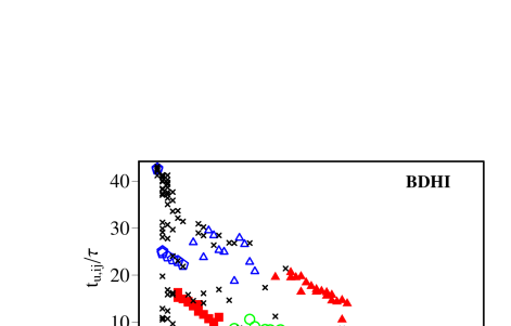
Figure 5:

Figure 6:

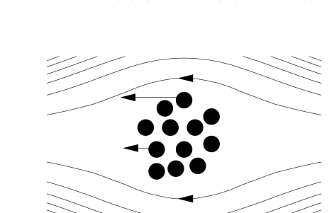
Figure 7:

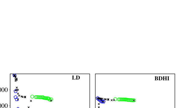
Figure 8:

References

- (1) J. K. G. Dhont, An Introduction to Dynamics of Colloids (Elsevier, Amsterdam, 1996).
- (2) R. G. Larson and J. J. Magda Macromolecules, 22, 3004 (1989).
- (3) H. Tanaka, J. Phys. Cond. Matt., 13, 4637 (2001).
- (4) E. Dickinson, Chem. Soc. Rev., 14, 421, (1985).
- (5) P. Wojtaszczyk and J. B. Avalos, Phys. Rev. Lett., 80, 754 (1998).
- (6) H. Tanaka, J. Phys. Cond. Matt., 17, S2795, (2005).
- (7) A. Baumketner and Y. Hiwatari, J. Phys. Soc. Jap., 71, 3069 (2002).
- (8) M. Carrion-Vazquez, H. B. Li, H. Lu, P. E. Marszalek, A. F. Oberhauser, and J. M. Fernandez, Nat. Struct. Biol. 10, 738, (2003).
- (9) C.-L. Chyan, F.-C. Lin, H. Peng, J.-M. Yuan, C.-H. Chang, S.-H. Lin and G. Yang, Biophys J., 87, 3995 (2004).
- (10) J. M. Fernandez and H. Li, Science 303 1674 (2004).
- (11) M. Schlierf, H. Li and J. M. Fernandez, Proc. Natl. Acad. Sci. (USA) 101, 7299, (2004).
- (12) D. Makarov, J. Phys. Chem. B., 108, 745 (2004).
- (13) P-C. Li and D. Makarov, J. Chem. Phys., 121, 4826 (2004).
- (14) M. Cieplak and P. E. Marszalek, J. Chem. Phys. 123 194903 (2005).
- (15) A. Irbäck, S. Mitternacht, and S. Mohanty, Proc. Natl. Acad. Sci. (USA) 102, 13427 (2005).
- (16) P. Szymczak and M. Cieplak, J. Phys.: Condens. Matter 18, L21, (2006).
- (17) D. K. West, D. J. Brockwell, P. D. Olmsted, S. R. Radford and E. Paci, Biophys. J., 90, 287, (2006).
- (18) H. Abe and N. Go, Biopolymers 20 1013 (1981); S. Takada, Proc. Natl. Acad. Sci. (USA) 96 11698 (1999).
- (19) M. Cieplak, T. X. Hoang and M. O. Robbins, Proteins: Struct. Funct. Bio. 56 285 (2004).
- (20) J. I. Sułkowska and M. Cieplak, J. Phys. Cond. Matt. (submitted).
- (21) H. Lu and K. Schulten, Chem. Phys. 247, 141 (1999).
- (22) J. Tsai, R. Taylor, C. Chothia, and M. Gerstein, J. Mol. Biol. 290 253 (1999).
- (23) M. Cieplak, A. Pastore and T. X. Hoang, J. Chem. Phys. 122 054906 (2004).
- (24) T. Veitshans, D. Klimov, and D. Thirumalai, Folding and Design, 2 1 (1997).
- (25) T. X. Hoang and M. Cieplak, J. Chem. Phys., 113, 8319 (2000).
- (26) H. A. Lorentz, Lectures on Theoretical Physics, Macmillan, London, 1927.
- (27) R. M. Mazo, Brownian Motion. Fluctuations, Dynamics, and Applications, Oxford Science, Oxford, 2002.
- (28) W. Min, G. Luo, B. J. Cherayil, S. C. Kou, and X.S. Xie, Phys. Rev. Lett, 94, 198302 (2005).
- (29) D. L. Ermak and J. A. McCammon, J. Chem. Phys., 69, 1352, (1978).
- (30) G. C. Anselle, E. Dickinson, and M. Ludvigsen, J. Chem. Soc., Faraday Trans. 81, 1269 (1985).
- (31) S. Kim and S. J. Karrila, Microhydrodynamics: Principles and Selected Applications, Butterworth-Heinemann, Boston, 1991.
- (32) P. Mazur and W. van Saarlos, Physica A, 115, 21 (1982).
- (33) L. Durlofsky, J. F. Brady, and G. Bossis, J. Fluid Mech., 180 21 (1987).
- (34) B. U. Felderhof, Physica A, 151, 16 (1988).
- (35) A. J. C. Ladd, J. Chem. Phys., 88, 5051, (1988).
- (36) B. Cichocki, B. U. Felderhof, K. Hinsen, E. Wajnryb, and J. Blawzdziewicz, J. Chem. Phys., 100, 3780, (1994).
- (37) T. N. Phung, J.F. Brady, and G. Bossis, J. Fluid Mech., 313, 181, (1996).
- (38) J. Rotne and S. Prager, J. Chem. Phys. 50, 4831, (1969).
- (39) H Yamakawa, J. Chem. Phys. 53 436 (1970).
- (40) E. Wajnryb, P. Szymczak, B. Cichocki, Physica A, 335, 339, (2004).
- (41) G. Nägele in Computational Condensed Matter Physics, ed.: S. Blügel, G. Gompper, E. Koch, H. Müller-Krumbhaar, R. Spatschek, R. G. Winkler, Forschungzentrum Jülich, B4:1, 2006.
- (42) P. Szymczak and M. Cieplak, J. Chem. Phys, 125, 164903, (2006).
- (43) A. Lemak, J. R. Lepock, and J. Z. Y. Chen, Proteins: Structure, Function and Genetics 51, 224 (2003).
- (44) A. Lemak, J. R. Lepock, J. Z. Y. Chen, Phys. Rev. E 67, 031910 (2003).
- (45) R. Rzehak, W. Kromen, T. Kawakatsu and W. Zimmermann, Europ. Phys. J. E 2, 3 (2000).