The theory of optical dispersive shock waves in photorefractive media

Abstract

The theory of optical dispersive shocks generated in propagation of light beams through photorefractive media is developed. Full one-dimensional analytical theory based on the Whitham modulation approach is given for the simplest case of sharp step-like initial discontinuity in a beam with one-dimensional strip-like geometry. This approach is confirmed by numerical simulations which are extended also to beams with cylindrical symmetry. The theory explains recent experiments where such dispersive shock waves have been observed.

I Introduction

Study of optical solitons is a large area of modern research which is important both scientifically and for potential applications (see, e.g., ka03 ; kld ). Different kinds of solitons have already been observed in various nonlinear optical media and their behavior has been explained in the frameworks of such mathematical models as nonlinear Schrödinger (NLS) and generalized nonlinear Schrödinger (GNLS) equations for different dimensions and geometries, so that one can consider the properties of single solitons as well enough understood.

However, there are situations when many solitons are generated so that they comprise a dense soliton lattice. In such situations, it is impossible to neglect interactions between solitons and one has to consider evolution of the structure as a whole rather than to trace evolution of each soliton separately. Usually, such soliton structures appear as a result of wave breaking of a large enough initial pulse or large disturbance along constant background. Hence, such structures can be considered as a dispersive counterparts of shock waves well known in physics of compressible viscous fluids (see, e.g., whitham-1 ). In a viscous fluid, the shock can be represented as a narrow region within which strong dissipation processes take place. In optics, on the contrary, dissipation effects can be neglected compared with dispersion ones and the shock discontinuity resolves into an expanding region filled with nonlinear oscillations. Such dispersive shock waves are known as tidal bores in rivers bl54 and have been also observed in some other physical systems including collisionless plasma plasma and Bose-Einstein condensate hoefer . Experiments on such dispersive shock waves production in optics have been recently reported in french ; fleischer . Motivated by these experiments, we shall consider here the theory of dispersive shock waves in photorefractive media.

Since the number of interacting solitons in dispersive shocks is usually much greater than unity and these solitons are spatially ranked in amplitude, such a dispersive shock can be represented as a modulated periodic wave with parameters changing a little in one transverse or longitudinal period of envelope amplitude of the electromagnetic wave. A slow change of the parameters of the envelope amplitude is governed to leading order by the Whitham modulation equations obtained by averaging conservation laws over the family of nonlinear periodic solutions or by the application of the averaged variational principle (see, e.g., whitham-1 ; ri ; kamch2000 ). For the one-dimensional NLS equation, the Whitham equations were derived in forest ; pavlov (see also kamch2000 ) and the mathematical theory of dispersive shock waves for the defocusing case was developed in gk87 ; eggk95 ; ek95 ; jin ; tian ; kku ; bk . It was applied to the propagation of signals in optical fibers in kodama and in Bose-Einstein condensates in kgk04 ; hoefer . It should be mentioned that for the case of the 1D NLS equation, the presence of an integrable structure has important consequences for the modulation (Whitham) system, namely, the latter can be represented in a diagonal (Riemann) form, which dramatically simplifies further analysis. The method of obtaining the Whitham equations in this form is based on the Inverse Scattering Transform (IST) applied to the NLS equation forest ,pavlov . However, in the case of the GNLS equation, the IST method cannot be used anymore, and the diagonal structure of the Whitham system is not available. Nevertheless, it was shown in el -ekt that in this case, the main characteristics of the dispersive shock wave still can be found by using some general properties of the Whitham equations which remain present even in non-integrable case. Here we shall use this latter method for derivation of parameters of one-dimensional dispersive shock waves generated in photorefractive crystals and shall confirm our analytical results by numerical simulations, which also provide a more detailed information in the cases when the analytical approach is not yet developed (say in 2D).

II Main equations

Photorefractive optical solitons were first observed in the experiment duree and in the experiments french ; fleischer the formation of dispersive shock waves has been observed in spatial evolution of light beams propagating through self-defocusing photorefractive crystals, so that beam non-uniformities give rise to breaking singularities and their resolution through dispersive shocks. As is known, propagation of such stationary beams is described by the equation

$$i\frac{\partial\psi}{\partial z}+\frac{1}{2k_{0}}\Delta_{\bot}\psi+\frac{k_{0}}{n_{0}}\delta n\left(|\psi|^{2}\right)\psi=0,$$ (1)

where $\psi$ is envelope field strength of electromagnetic wave with wave number $k_{0}=2\pi n_{0}/\lambda$, $z$ is the coordinate along the beam, $x,y$ are transverse coordinates, ${\bf r}=(x,y)$, $\Delta_{\bot}=\partial^{2}/\partial^{2}x+\partial^{2}/\partial^{2}y$ is transverse Laplacian, $n_{0}$ is a linear refractive index, and in photo-refractive medium we have

$$\delta n=-\frac{1}{2}n_{0}^{3}r_{33}E_{p}\frac{\rho}{\rho+\rho_{d}},$$ (2)

where $E_{p}$ is applied electric field, $r_{33}$ electro-optical index, $\rho=|\psi|^{2}$, and $\rho_{d}$ is a saturation parameter.

For mathematical convenience, we introduce non-dimensional variables

$$\tilde{z}=\frac{1}{2}kn_{0}^{2}r_{33}E_{p}\left(\frac{\rho_{c}}{\rho_{d}}\right)z,\quad\tilde{x}=kn_{0}\sqrt{\frac{1}{2}r_{33}E_{p}\left(\frac{\rho_{c}}{\rho_{d}}\right)}x,\quad\tilde{y}=kn_{0}\sqrt{\frac{1}{2}r_{33}E_{p}\left(\frac{\rho_{c}}{\rho_{d}}\right)}y,\quad\tilde{\psi}=\sqrt{\rho_{c}}\psi,$$ (3)

where $\rho_{c}$ is a characteristic value of optical intensity (its concrete definition depends on the problem under consideration; for instance, it can the background intensity), so that Eq. (1) takes the form of GNLS equation

$$i\frac{\partial\psi}{\partial z}+\frac{1}{2}\Delta_{\bot}\psi-\frac{|\psi|^{2}}{1+\gamma|\psi|^{2}}\psi=0,$$ (4)

where $\gamma=\rho_{c}/\rho_{d}$ and tildes are omitted. If saturation effect is negligibly small ($\gamma|\psi|^{2}\ll 1$), then this equation reduces to the usual NLS equation

$$i\frac{\partial\psi}{\partial z}+\frac{1}{2}\Delta_{\bot}\psi-{|\psi|^{2}}\psi=0.$$ (5)

It is convenient to represent these equations in a fluid dynamics type form by means of the substitution

$$\psi({\bf r},z)=\sqrt{\rho}\,\exp\left(i\int^{{\bf r}}{\bf u}({\bf r},z)d{\bf r}\right),$$ (6)

so that they are transformed to

$$\begin{split}\rho_{z}+\nabla_{\bot}(\rho{\bf u})=0,\\ {\bf u}_{z}+\left({\bf u}\nabla_{\bot}\right){\bf u}+\nabla_{\bot}f(\rho)-\nabla_{\bot}\left[\frac{\Delta_{\bot}\rho}{4\rho}-\frac{(\nabla_{\bot}\rho)^{2}}{8\rho^{2}}\right]=0,\end{split}$$ (7)

where

$$f(\rho)=\frac{\rho}{1+\gamma\rho}\qquad\textrm{ for the GNLS equation (\ref{1-5})}$$ (8)

and

$$f(\rho)={\rho}\qquad\textrm{ for the NLS equation (\ref{1-6})}\,.$$ (9)

The light intensity $\rho$ in the hydrodynamic interpretation has a meaning of a density of a “fluid” and Eqs. (8), (9) can be viewed as “equations of state” for such a fluid. The function ${\bf u}({\bf r},z)$ is a local value of the wave vector component transverse to the direction of the light beam; in hydrodynamic representation it has a meaning of the “flow velocity”. The variable $z$ plays the role of time so it is natural to describe the deformations of the light beam in evolutionary terms. Obviously, if initial distribution does not depend on one of the transverse coordinates (say $y$), then transverse differential vector operators reduce to usual derivatives ($\nabla_{\bot}=\partial/\partial x$, $\Delta_{\bot}=\partial^{2}/\partial x^{2}$).

Evolution, according to (7) of an initial distribution, specified at $z=0$, typically leads to wave breaking and formation of dispersive shock waves. One can distinguish the following typical cases:

• generation of dispersive shocks in the evolution of a bright strip hump above a uniform (background) intensity distribution,

• generation of sequences of solitons from a strip “hole” in the light intensity,

• generation of dispersive shocks in the evolution of a bright cylindrically symmetrical hump above a uniform intensity distribution.

In 1D geometry such humps can be modeled qualitatively by step-like pulses with sharp boundaries, and these models are convenient for analytical considerations. As was shown in hoefer for the NLS equation case with $\gamma=0$, this model agrees quite well with numerical simulations of 2D dynamics. Therefore we shall start here with these idealized models.

III Analytical theory of one-dimensional dispersive shocks generated in decay of a step-like initial distribution

We shall start with analytical treatment of shocks described by 1D equation

$$i\psi_{z}+\frac{1}{2}\psi_{xx}-f(|\psi|^{2})\psi=0,$$ (10)

or, in a fluid dynamics form, by the system

$$\begin{split}\rho_{z}+(\rho u)_{x}=0,\\ u_{z}+uu_{x}+\frac{df}{d\rho}\rho_{x}+\left(\frac{(\rho_{x})^{2}}{8\rho^{2}}-\frac{\rho_{xx}}{4\rho}\right)_{x}=0,\end{split}$$ (11)

where the nonlinear refraction function $f(\rho)$ is given by Eq. (8) or (9). The systems of the type (11) are often referred to as dispersive hydrodynamics systems.

We consider initial distributions of the intensity and transverse wave vector in the form

$$\rho(x,0)=\left\{\begin{array}[]{ll}\rho_{0}&\quad\hbox{for}\quad x<0,\\ 1&\quad\hbox{for}\quad x\geq 0;\end{array}\right.\qquad u(x,0)=0,$$ (12)

that is we assume that the initial velocity $u(x,0)$ is equal to zero everywhere which means that the initial beam enters the photo-refractive medium at $z=0$ without any focusing. For the sake of definiteness we assume also that $\rho_{0}>1$.

At the initial stage of evolution, linear waves are generated which propagate according to the dispersion law obtained by means of linearization of Eqs. (11) about the uniform state $\rho=\rho_{0}$, $u=u_{0}$ (we keep here a nonzero value of $u_{0}$ for future convenience), that is $\rho=\rho_{0}+\rho_{1}\exp[i(kx-\omega z)]$, $u=u_{0}+u_{1}\exp[i(kx-\omega z)]$, where $\rho_{1},\,u_{1}\ll 1$. Then a simple calculation yields

$$\omega=\omega_{0}(\rho_{0},u_{0},k)=ku_{0}\pm k\sqrt{\frac{\rho_{0}}{(1+\gamma\rho_{0})^{2}}+\frac{k^{2}}{4}}\,.$$ (13)

Note that $\omega^{\prime\prime}(k)>0$, which implies appearance of dark solitons in full nonlinear solutions. But before consideration of such solutions, we shall discuss a nonlinear stage of evolution in dispersionless approximation when one can neglect the higher order terms in the system (11). While in the case of general smooth initial data this stage of evolution is responsible for the formation of breaking singularities in the solution, its consideration also provides important insights into the nonlinear dissipationless dispersive dynamics of discontinuous disturbances of the type (12) even beyond the breaking point.

III.1 Dispersionless approximation

In dispersionless approximation, the system (11) reduces to standard equations of compressible fluid dynamics

$$\begin{split}\rho_{z}+(\rho u)_{x}=0,\\ u_{z}+uu_{x}+{f^{\prime}(\rho)}\rho_{x}=0.\end{split}$$ (14)

Because of the bi-directional nature of this system, generally, an initial step (12) resolves into a combination of two waves propagating in opposite directions. One of these waves represents a rarefaction wave with clear physical meaning, but the other one leads to a multi-valued dependence of the intensity $\rho(x,z)$ and transverse wave number (associated flow velocity) $u(x,z)$ on the $x$–coordinate. Nevertheless, this formal global solution sheds some light on the structure of the actual physical solution and some its elements will be used later, therefore we shall consider it here. To this end we cast the system (14) into a diagonal form (see, for instance, whitham-1 ; kamch2000 ) by introduction of new variables—Riemann invariants

$$r_{\pm}=u\pm\frac{2}{\sqrt{\gamma}}\arctan\sqrt{\gamma\rho},$$ (15)

so that it takes the form

$$\frac{\partial r_{\pm}}{\partial z}+V_{\pm}\frac{\partial r_{\pm}}{\partial x}=0,$$ (16)

where the characteristic velocities $V_{\pm}$ are expressed in terms of the hydrodynamic variables $\rho,u$ by the relationships

$$\qquad V_{\pm}=u\pm\frac{\sqrt{\rho}}{1+\gamma\rho}.$$ (17)

When $\gamma\to 0$ we have $r_{\pm}=u\pm 2\sqrt{\rho}$, $V_{\pm}=u\pm\sqrt{\rho}$, i.e. the usual expressions for the dispersionless limit of the defocusing NLS equation (the shallow-water system—see, for instance, gk87 ).

Since in the case of the step-like initial conditions the variables $r_{\pm}$ must depend on a self-similar variable $\zeta=x/z$ alone, the equations Eqs. (16) reduce to $(V_{\pm}-\zeta)(dr_{\pm}/d\zeta)=0$ and we arrive at the so-called simple-wave solutions:

$$u+\frac{\sqrt{\rho}}{1+\gamma\rho}=\frac{x}{z},\qquad u-\frac{2}{\sqrt{\gamma}}\arctan\sqrt{\gamma\rho}=r_{-}^{0}=\mathrm{constant},$$ (18)

or

$$u-\frac{\sqrt{\rho}}{1+\gamma\rho}=\frac{x}{z},\qquad u+\frac{2}{\sqrt{\gamma}}\arctan\sqrt{\gamma\rho}=r^{0}_{+}=\mathrm{constant}.$$ (19)

The constants here are chosen from the continuity conditions at the points where the simple waves enter the regions of constant intensities. Since the left-propagating rarefaction wave described by (19) matches with the external flow $\rho=\rho_{0}$, $u=0$ (see Fig. 1a) we have $r_{+}^{0}=\frac{2}{\sqrt{\gamma}}\arctan\sqrt{\gamma\rho_{0}}$ and, correspondingly

$$u=\frac{2}{\sqrt{\gamma}}\left({\arctan\sqrt{\gamma\rho_{0}}}-\arctan{\sqrt{\gamma\rho}}\right).$$ (20)

Now, substituting this into the first equation (19) we get

$$\frac{\sqrt{\rho}}{1+\gamma\rho}+\frac{2}{\sqrt{\gamma}}\left(\arctan{\sqrt{\gamma\rho}}-\arctan{\sqrt{\gamma\rho_{0}}}\right)=-\frac{x}{z}\,,$$ (21)

which determines implicitly the intensity $\rho$ as a function of $x/z$ in the rarefaction wave. For $x<x_{1}^{-}$ we have $\rho=\rho_{0}=\mathrm{constant}$ so $x=x_{1}^{-}$ is the point of weak discontinuity which must propagate with sound velocity (see, for instance lanlif ) which in our case is

$$c_{s}(\rho)=\frac{\sqrt{\rho}}{1+\gamma\rho},$$ (22)

Indeed, substituting $\rho=\rho_{0}$ into (21) we get $x^{-}_{1}/z=-c_{s}(\rho_{0})$. As a matter of fact, the speeds of propagation of weak discontinuities in the photorefractive system agree with the group speeds determined by the long wavelength limit $k\to 0$ in the linear dispersion relation (13).

Next, for $x>x_{2}^{-}$ we have $\rho=1$, $u=0$ (see Fig. 1a) and this does not agree with the relationship (20) in the constructed left-propagating rarefaction wave solution. Hence, we have to introduce some intermediate distribution

$$\rho(x/z)=\rho^{-}=\mathrm{constant},\quad u(x/z)=u^{-}=\mathrm{constant}$$ (23)

which matches with the rarefaction wave at some $x=x_{1}^{+}$. Now, to connect the intermediate distribution (23) with $\rho=1$, $u=0$ downstream, we have to use the right-propagating simple wave solution (18) where the constant $r^{0}_{+}=\frac{2}{\sqrt{\gamma}}\arctan\sqrt{\gamma}$. Hence we get

$$u=\frac{2}{\sqrt{\gamma}}\left({\arctan\sqrt{\gamma\rho}}-\arctan{\sqrt{\gamma}}\right)$$ (24)

and

$$\frac{\sqrt{\rho}}{1+\gamma\rho}+\frac{2}{\sqrt{\gamma}}\left({\arctan\sqrt{\gamma}}-\arctan{\sqrt{\gamma\rho}}\right)=\frac{x}{z}\,.$$ (25)

Equations (20) and (24) at $\rho=\rho^{-}$ must give $u=u^{-}$; hence they yield the equation

$$\arctan\sqrt{\gamma\rho^{-}}=\frac{1}{2}\left(\arctan\sqrt{\gamma\rho_{0}}+\arctan\sqrt{\gamma}\right)$$ (26)

which determines the parameter $\rho^{-}$:

$$\rho^{-}=\left[\frac{\sqrt{1+\gamma\rho_{0}}-1+\sqrt{\rho_{0}}(\sqrt{1+\gamma}-1)}{\gamma\sqrt{\rho_{0}}-(\sqrt{1+\gamma\rho_{0}}-1)(\sqrt{1+\gamma}-1)}\right]^{2}.$$ (27)

When $\rho^{-}$ is known, the parameter $u^{-}$ is found from the equation (24),

$$u^{-}=\frac{2}{\sqrt{\gamma}}\left({\arctan\sqrt{\gamma\rho^{-}}}-\arctan{\sqrt{\gamma}}\right).$$ (28)

The “internal” end points $x_{1}^{+}$ and $x_{2}^{-}$ are found by substituting the intermediate values $\rho^{-}$, $u^{-}$ into the similarity solutions (18), (19),

$$\frac{x_{1}^{+}}{z}=u^{-}-\frac{\sqrt{\rho^{-}}}{1+\gamma\rho^{-}},\qquad\frac{x_{2}^{-}}{z}=u^{-}+\frac{\sqrt{\rho^{-}}}{1+\gamma\rho^{-}}.$$ (29)

These points correspond to the weak discontinuities which propagate with sound velocities $c_{s}(\rho^{-})$ in opposite directions in the reference frame associated with the uniform flow $u^{-}$.

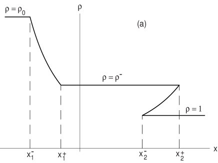
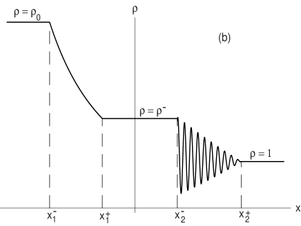
Figure 1: Decay of the initial discontinuity of light intensity in a beam propagating through a photorefractive crystal. (a) Dispersionless approximation with non-physical region of multi-valued intensity. (b) Schematic picture of formation of dispersive shock due to interplay of dispersive and nonlinear effects. The values of $x_{1}^{-}$ and $x_{1}^{+}$ are the same for (a) and (b) while the values of $x_{2}^{-}$ and $x_{2}^{+}$ are different.

The whole structure of intensity distribution is shown in Fig. 1a. It has the region $x_{2}^{-}<x<x_{2}^{+}$ with the three-valued intensity, corresponding to the formal solution (18), which is obviously non-physical and its appearance serves as an indication that an oscillating dispersive shock wave is generated in the region of transition from $\rho=\rho^{-},\,u=u^{-}$ to $\rho^{+}=1,\,u^{+}=0$. The arising physical structure is shown schematically in Fig. 1b. Importantly, the boundaries $x_{1,2}$ of the oscillatory zone by no means coincide with those in the formal three-valued dispersionless solution. It is remarkable, however, that in spite of such radical qualitative and quantitative change of the flow, the values of $\rho^{-}$ and $u^{-}$ themselves turn out to be still determined by the previous equations (27) and (28). This is a consequence of the dispersive shock jump condition which requires that the values of the Riemann invariant $r_{-}=u-(2/\sqrt{\gamma})\arctan\sqrt{\gamma\rho}$ at both end points of the dispersive shock wave must be equal to each other:

$$\left.r_{-}\right|_{x_{2}^{-}}=\left.r_{-}\right|_{x_{2}^{+}}\,,$$ (30)

which gives at once Eq. (28). Since the rarefaction wave, even in the presence of dispersion, is still described with good accuracy by the dispersionless approximation (see gp74 , gm84 for the general linear asymptotic analysis of the dispersive resolution of the weak discontinuities at the edges of the rarefaction wave), we deduce that Eq. (27) obtained in the framework of the dispersionless fluid dynamics also remains valid. One should emphasize that, although all obtained relationships, strictly speaking, hold only asymptotically for sufficiently large “times” $z$, as we shall see from the direct numerical solution, they hold with good accuracy for rather moderate $z$. The dispersive jump condition of the type (30) was proposed for the first time in gm84 where it was based on intuitive physical reasoning and the results of numerical simulations of collisionless plasma flows. A consistent mathematical derivation of this condition along with some important restrictions to its applicability was given in the framework of the Whitham theory in el ; ekt .

As was mentioned, the end points of the oscillatory region of the dispersive shock in Fig. 1b do not coincide with the end points of the three-valued region in Fig. 1a. Indeed, this oscillatory zone arises due to interplay of dispersion and nonlinear effects and has a structure similar to that observed in the much studied integrable defocusing NLS equation case (see gk87 -kgk04 ). Namely, near the leading edge $x_{2}^{+}$ the wave transforms into a vanishing amplitude linear wavepacket and at the trailing edge $x_{2}^{-}$ it converts into a dark soliton. Hence, the end point of the oscillatory zone $x_{2}^{+}$ must move with the group velocity of linear waves $c_{g}=\partial\omega_{0}/\partial k$ calculated for some non-zero value of $k=k^{+}$ in contrast to the dispersionless approximation corresponding to $k\to 0$ (in addition to vanishing amplitude of oscillations $a\to 0$). The end point $x_{2}^{-}$ moves with the corresponding soliton velocity which also has nothing to do with the dispersionless limit (note, that in the soliton limit $k\to 0$ but the amplitude $a=a^{-}$ remains finite). Thus, our task is to determine the main quantitative characteristics of the oscillatory region of the dispersive shock—the velocities of its end points as well as the amplitude $a^{-}$ of the trailing soliton at $x=x_{2}^{-}$ and the wave number $k^{+}$ at the leading edge point $x=x_{2}^{+}$.

One can observe that the oscillatory structure of the dispersive shock wave is characterized by two different spatial scales: the intensity oscillates very fast inside the shock but the parameters of the fast oscillations change little in one wavelength in $x$-direction and in one period along the beam $z$-axis. This suggests that the oscillatory dispersive shock can be represented as a slowly modulated nonlinear periodic wave and, hence, we can apply the Whitham modulation theory whitham-1 to its description. In the Whitham approach, the original equation containing higher order $x$-derivatives is averaged over the family of nonlinear periodic traveling wave solutions. As a result, one obtains a system of the first order nonlinear partial differential equations of hydrodynamic type (i.e. linear with respect to first derivatives) governing the slow evolution of modulations. The modulation system does not contain any parameters of the length dimension, so it allows one to introduce the edges $x^{\pm}_{2}(z)$ of the dispersive shock wave in a mathematically consistent way, as characteristics where matching of the “internal” (modulation) and “external” (dispersionless fluid dynamics) solutions occurs. Of course, strictly speaking the averaged description is valid only when the ratio of the typical wavelength to the width of the oscillatory zone is small. For our case of the decay of an initial discontinuity this corresponds to a “long-time” asymptotic behaviour, $z\gg 1$. However, as we shall see from the comparison with direct numerical solution, the results of the modulation approach turn out to be valid even for rather moderate values of $z$.

The modulation approach to the description of dispersive shock waves was realized for the first time by Gurevich and Pitaevskii gp74 in the framework of the Korteweg – de Vries equation. To put this approach into practice for the light beam deformations in a photorefractive medium, we first have to study periodic solutions of the equations (11).

III.2 Periodic waves and solitons in photorefractive crystals

The traveling wave solution of the system (11) is obtained by the substitution $\rho=\rho(\theta)$, $u=u(\theta)$, where $\theta=x-cz$ is the phase and $c=\hbox{constant}$ is the phase velocity. As a result, we obtain by integrating the first equation (11)

$$u=c+\frac{A}{\rho},$$ (31)

where $A$ is an arbitrary constant. Substituting (31) into the second equation (11) and performing one integration with respect to $\theta$ we obtain an ordinary differential equation of the second order,

$$\frac{1}{8}\left(\frac{d\rho}{d\theta}\right)^{2}=\frac{1}{4}\frac{d^{2}\rho}{d\theta^{2}}\rho-\rho^{2}f(\rho)-B\rho^{2}-\frac{A^{2}}{2},$$ (32)

where $B$ is another constant of integration. We shall seek its integral in the form

$$\left(\frac{d\rho}{d\theta}\right)^{2}=a_{1}\rho\int f(\rho)d\rho+a_{2}\rho^{2}+a_{3}\rho+a_{4},$$ (33)

where $a_{1}$, $a_{2}$, $a_{3}$, and $a_{4}$ are the constant coefficients to be found. Substituting (33) into (32) we find, with the account of the specific dependence $f(\rho)$, the eventual form of the sought integral,

$$\left(\frac{d\rho}{d\theta}\right)^{2}=-\frac{8\rho}{\gamma^{2}}\ln(1+\gamma\rho)+\left(a_{2}+\frac{8}{\gamma}\right)\rho^{2}+a_{3}\rho+a_{4}\equiv Q(\rho).$$ (34)

Here $a_{2}$, $a_{3}$ and $a_{4}$ are arbitrary constants two of which are connected with $A$ and $B$ by the relations

$$a_{2}=8B,\quad a_{4}=-4A^{2},$$ (35)

and $a_{3}$ is an additional constant so that (34) is indeed the first integral of Eq. (32). We denote the roots of the equation $Q(\rho)=0$ as $e_{1}\leq e_{2}\leq e_{3}$. Then the density oscillations in the traveling wave occur between $e_{1}$ and $e_{2}$. The amplitude of the wave is then given by $a=e_{2}-e_{1}$. The small-amplitude linear wave configuration corresponds to $e_{1}\to e_{2}$ while for solitons we have $e_{2}=e_{3}$. By imposing the periodicity condition $\rho(\theta)=\rho(\theta+2\pi/k)$ we find the wave number $k$ of the traveling wave in the form of the integral

$$k=\pi\left(\int_{e_{1}}^{e_{2}}\frac{d\rho}{\sqrt{Q(\rho)}}\right)^{-1}.$$ (36)

While the equation (34) cannot be integrated in closed form, it is not difficult to find the relationships characterizing its special solution in the form of a dark soliton. For this solution we must have the following boundary conditions satisfied at infinity:

$$\rho\to\rho_{b},\quad u\to u_{b},\quad d\rho/d\theta\to 0,\quad d^{2}\rho/d\theta^{2}\to 0\qquad\text{for}\quad|\theta|\to\infty,$$ (37)

plus the condition $d\rho/d\theta=0$ at $\rho=\rho_{m}\leq\rho_{b}$, where $\rho_{m}$ is the value of the “density” in the minimum of the dark soliton and $\rho_{b}$ is the “background” intensity. Applying these conditions to (31), (34) we obtain, after simple algebra, the expressions for the coefficients in (34) for the soliton configuration,

$$\begin{split}a_{2}&=-\frac{8\rho_{b}}{1+\gamma\rho_{b}}-4(u_{b}-c)^{2},\\ a_{3}&=\frac{8}{\gamma^{2}}\ln(1+\rho_{b})-\frac{8\rho_{b}}{\gamma(1+\gamma\rho_{b})}+\frac{4(u_{b}-c)^{2}(\rho_{m}^{2}+\rho_{b}^{2})}{\rho_{b}},\\ a_{4}&=-4(u_{b}-c)^{2}\rho_{b}^{2}.\end{split}$$ (38)

The curves $Q(\rho)$ in a “soliton configuration” for several values of $\gamma$ are shown in Fig. 2.

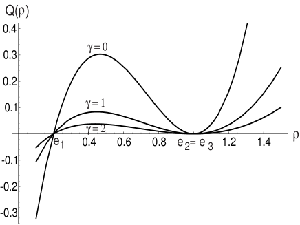
Figure 2: Plots of the function $Q(\rho)$ corresponding to $\rho_{b}=1$, $\rho_{m}=0.2$ and different values of $\gamma$ and $\rho_{b}=1,$ $\rho_{m}=0.2,$ so that $e_{1}=0.2,$ $e_{2}=e_{3}=1$.

The condition that in the soliton limit $\rho_{b}$ is a double zero of the function $Q(\rho)$, that is $dQ(\rho)/d\rho=0$ at $\rho=\rho_{b}$, yields the relationship between the soliton velocity $c$ and the amplitude $a=\rho_{b}-\rho_{m}$ for given $\rho_{b}$, $u_{b}$:

$$(c-u_{b})^{2}=\frac{2\rho_{m}}{\gamma a}\left[\frac{1}{\gamma a}\ln\frac{1+\gamma\rho_{b}}{1+\gamma\rho_{m}}-\frac{1}{1+\gamma\rho_{b}}\right].$$ (39)

The dependence of the soliton velocity on the saturation parameter $\gamma$ is shown in Fig. 3.

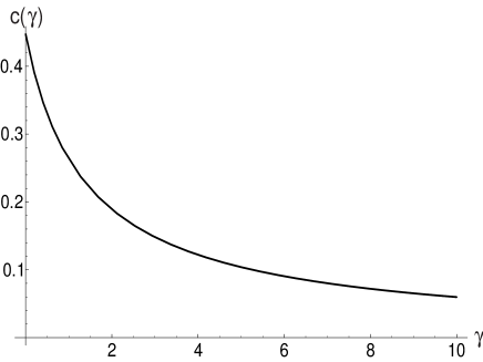
Figure 3: The plot of soliton velocity as a function of the saturation parameter $\gamma$. The other parameters are: $\rho_{b}=1$, $\rho_{m}=0.2$.

For future analysis it is important to introduce one more parameter—the inverse half-width $\kappa$ of the soliton— using the exponential decay of the intensity $\rho_{b}-\rho$ as $|\theta|\to\infty$:

$$\rho_{b}-\rho\propto\exp(-\kappa|\theta|),\quad|\theta|\to\infty.$$ (40)

To find the relationship between $\kappa$ and other parameters we take the series expansion of $Q(\rho)$ for small values of $\rho^{\prime}=\rho_{b}-\rho$ and find $(d\rho^{\prime}/d\theta)^{2}=(1/2)(d^{2}Q/d\rho^{2})_{\rho_{b}}(\rho^{\prime})^{2}=\kappa^{2}(\rho^{\prime})^{2}$; hence

$$\kappa=\left(\frac{1}{2}\left.\frac{d^{2}Q}{d\rho^{2}}\right|_{\rho_{b}}\right)^{1/2}=\left[\frac{8\rho_{m}+4\gamma\rho_{b}(\rho_{b}+\rho_{m})}{\gamma(\rho_{b}-\rho_{m})(1+\gamma\rho_{m})^{2}}-\frac{8\rho_{m}}{\gamma^{2}(\rho_{b}-\rho_{m})^{2}}\ln\frac{1+\gamma\rho_{b}}{1+\gamma\rho_{m}}\right]^{1/2}.$$ (41)

The dependence of $\kappa$ on $\gamma$ is shown in Fig. 4.

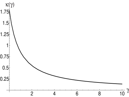
Figure 4: The plot of inverse half-width $\kappa$ of photorefractive soliton as a function of saturation parameter $\gamma$. The other parameters are: $\rho_{b}=1$, $\rho_{m}=0.2$.

The profile of the intensity $\rho(\theta)$ is determined by the integral (see Eq. (34))

$$\theta=\int_{\rho_{m}}^{\rho}\frac{d\rho}{\sqrt{Q(\rho)}},$$ (42)

where it is assumed that the intensity $\rho$ takes the minimal value $\rho=\rho_{m}$ at $\theta=0$ which determines the integration constant. The wave form of a dark soliton for different values of the parameter $\gamma$ is shown in Fig. 5.

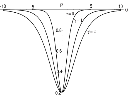
Figure 5: Profiles of the intensity in photorefractive solitons for values of $\gamma=0,\,1,\,2$. The other parameters are: $\rho_{b}=1$, $\rho_{m}=0.2$.

For $\gamma\ll 1$ we have asymptotic expansions (for simplicity we take $u_{b}=0$)

$$c=\sqrt{\rho_{m}}\left(1-\frac{\gamma}{3}(2\rho_{b}+\rho_{m})\right)+\mathcal{O}(\gamma^{2}).$$ (43)

$$\kappa=2\sqrt{\rho_{b}-\rho_{m}}\left[1-\frac{\gamma}{3}(3\rho_{b}+\rho_{m})\right]+\mathcal{O}(\gamma^{2}),$$ (44)

and for $\gamma\gg 1$ other expansions

$$c=\frac{\sqrt{2[\rho_{m}(\ln(\rho_{b}/\rho_{m})-1)+\rho_{m}^{2}/\rho_{b}]}}{(\rho_{b}-\rho_{m})\gamma}+\mathcal{O}(\gamma^{-2}),$$ (45)

$$\kappa=\frac{2\sqrt{\rho_{b}-2\rho_{m}\ln(\rho_{b}/\rho_{m})-\rho_{m}^{2}/\rho_{b}}}{(\rho_{b}-\rho_{m})\gamma}+\mathcal{O}(\gamma^{-3}).$$ (46)

One can see that the leading terms in (43) and (44) agree with the well-known dependencies for dark solitons of the NLS equation gk87 .

The particular case of soliton solution with $\rho_{m}=0$, $u_{b}=0$ (hence $c=0$) in photorefractive media has been found in hou .

III.3 Dispersive shock wave

The general periodic solution of the photorefractive equation depends on the fast phase variable $\theta$ and is characterized by four parameters $e_{1},\,e_{2},\,e_{3},c$, where $e_{j},\ j=1,2,3$ are the zeroes of the function $Q(\rho)$ (34), which determine the profile of the intensity, and $c$ is the phase velocity. In a modulated wave, these four parameters become slow variables of $x$ and $z$. In the Whitham theory whitham-1 , it is postulated that this slow evolution (modulation) $e_{j}(x,z)$, $c(x,z)$ can be found from the conservation laws of the dispersive equation averaged over fast oscillations with respect to the phase variable $\theta$. An additional modulation equation naturally arises as the wave number conservation law $k_{z}+\omega_{x}=0$ and essentially represents a condition of the existence of a slowly modulated periodic wave (see, for instance, whitham-1 ). Several averaging procedures have been proposed yielding equivalent results for various physical systems (see ri ) so the Whitham modulation theory can be now considered as quite well established. As a result, using the original procedure of averaging conservation laws, the Whitham system for the GNLS equation can be obtained in the following general form

$$(\overline{P_{i}}(e_{1},e_{2},e_{3},c))_{z}+(\overline{Q_{i}}(e_{1},e_{2},e_{3},c))_{x}=0\,,\qquad i=1,2,3,$$ (47)

$$(k(e_{1},e_{2},e_{3},c))_{z}+(\omega(e_{1},e_{2},e_{3},c))_{x}=0\,,\qquad\omega=kc.$$ (48)

Here $P_{1}=\rho$, $P_{2}=u$, $P_{3}=\rho u$ are the conserved “densities” of the GNLS equation (7) and $Q_{i},\ i=1,2,3,$ are the corresponding “fluxes”. The averaging is performed over the periodic family (31), (34) according to

$$\overline{f}(e_{1},e_{2},e_{3},c)=\frac{k}{\pi}\int\limits_{e_{1}}^{e_{2}}\frac{f(\rho;e_{1},e_{2},e_{3},c)}{\sqrt{Q(\rho)}}d\rho\,.$$ (49)

Now the system (47), (48) is, in principle, completely defined.

The modulation system (47), (48) being the system of hydrodynamic type can be hyperbolic (real characteristic velocities – modulationally stable case) or elliptic (complex characteristic velocities – modulationally unstable case). It is known very well (see forest , pavlov , kamch2000 ) that for the defocusing NLS equation, which is an integrable particular case of the the GNLS equation (4), the modulation system is strictly hyperbolic. Our numerical simulations show that traveling waves in the GNLS equation are modulationally stable and this suggests that the corresponding Whitham system is hyperbolic as well. So, in what follows, we shall assume hyperbolicity of the Whitham system, which will allow us to use some arguments of classical characteristics theory lanlif ; courant ; whitham-1 .

Now, to describe analytically the dispersive shock wave as a whole, we have to solve four modulation equations (47), (48) for the slowly varying parameters $e_{1},e_{2},e_{3}$ and $c$ of the periodic solution. These equations must be equipped with special matching conditions to guarantee continuity of the mean flow at the free boundaries $x^{\pm}(z)$ defining the edges of the dispersive shock wave. In view of the numerically established qualitative spatial structure of the photorefractive dispersive shock wave (see Fig. 1b) we require that

$$\hbox{at}\quad x=x^{+}(z):\qquad a=0\,,\quad\overline{\rho}=\rho^{+}\,,\quad\overline{u}=u^{+}\,,$$ (50)

$$\hbox{at}\quad x=x^{-}(z):\qquad k=0\,,\quad\overline{\rho}=\rho^{-}\,,\quad\overline{u}=u^{-}\,,$$ (51)

where $x^{+}\equiv x_{2}^{+}$ (from now on we shall omit the subscript 2 in $x_{2}^{-}$ and $x_{2}^{+}$). The dependencies of $\overline{\rho}$, $\overline{u}$, $k$, $a$ on $e_{1},e_{2},e_{3},c$ are defined by (49) and formulae of Section III.B, and the pairs $(\rho^{-}$, $u^{-})$ and $(\rho^{+}$, $u^{+})$ represent the solution of the dispersionless approximation (14) evaluated at the trailing and leading edges of the dispersive shock wave respectively. The edges $x^{\pm}(z)$ of the dispersive shock wave represent free boundaries defined by the kinematic boundary conditions with clear physical meaning explained in Section III.A:

$$\frac{dx^{+}}{dz}=c_{g}(\rho^{+},u^{+},k^{+})\,,\qquad\frac{dx^{-}}{dz}=c_{sol}(\rho^{-},u^{-},a^{-})\,,$$ (52)

where $c_{g}(\rho^{+},u^{+},k)=\partial\omega_{0}/\partial k$ is the group velocity of the linear wave packet with the dominant wavenumber $k$ propagating against the hydrodynamic background $\rho^{+}$, $u^{+}$ (see (13) for the linear dispersion relation $\omega=\omega_{0}(\rho_{0},u_{0},k)$) and $c_{sol}(\rho^{-},u^{-},a)$ is the velocity of the dark soliton with amplitude $a$ propagating against the background $\rho^{-}$, $u^{-}$ (see (39) for the dependence of the soliton velocity on its amplitude). Of course, the values of the wavenumber $k^{+}$ at the leading edge and the amplitude $a^{-}$ of the trailing dark soliton are both to be determined, so the determination of the edges $x^{\pm}(z)$ represents a part of this nonlinear boundary value problem.

Following the pioneering work of Gurevich and Pitaevskii gp74 on the dispersive shock wave description in the framework of the KdV equation, the effective methods for treatment of such problems have been developed for the whole class of evolution equations which share with the KdV equation the unique property of complete integrability (see, e.g., kamch2000 ). On the level of the Whitham equations, one of the manifestations of integrability is the presence of the full system of Riemann invariants, an event generally highly unlikely for the systems of hydrodynamic type with number of equations exceeding two. In particular, the NLS equation (5) belongs to this class, and the corresponding theory of dispersive shock formation was developed in the papers gk87 ; eggk95 ; ek95 ; jin ; tian ; kku ; bk and successfully applied to the description of shocks in nonlinear optics kodama and Bose-Einstein condensates kgk04 ; hoefer . However, the photorefractive equation (4) is not completely integrable and therefore the methods based on the presence of rich underlying algebraic structure of such equations cannot be applied here. Nevertheless, as was shown in el -ekt , the main quantitative characteristics of the dispersive shock wave can be derived using the general properties of the Whitham equations (47), (48) reflecting their origin as certain averages, and here we shall apply this method to the description of dispersive shock waves in photorefractive media. To be specific, we shall be interested in the locations of the edges of the dispersive shock wave and in the amplitude of the largest (deepest) soliton at the trailing edge, the parameters that are usually observed in experiment.

The method of Refs. el -ekt , which will be used below, is formulated most conveniently in terms of the physical modulation parameters $\overline{\rho},\,\overline{u},\,k,\,a$ appearing in the matching conditions (51), (50). The key of the method lies in the fact that the modulation system (47), (48) dramatically simplifies in the cases ($a=0,\ k\neq 0$) and ($k=0,\ a\neq 0$) corresponding to the limiting wave regimes realized at the boundaries of the dispersive shock wave.

III.3.1 Leading edge

At the leading edge $x=x^{+}(z)$ the amplitude of oscillations vanishes, $a=0$. Since the Whitham averaging procedure remains valid for the case $a=0$ (averaging over the periodic family with vanishing amplitude), then we conclude that the Whitham system must admit an exact reduction at $a=0$ and, therefore, the system of four Whitham equations must reduce here to only three equations. Now, if the amplitude of oscillations vanishes, then the average of a function of the oscillating variable equals to the same function of the averaged variable: $\overline{F(\rho,u)}=F(\overline{\rho},\overline{u})$. Thus, when $a=0$ the Whitham system must agree with the dispersionless approximation (14) describing large-scale non-oscillating flows, i.e. the modulation equations for $\bar{\rho}$, $\bar{u}$, $a$ reduce to

$$a=0,\qquad\overline{\rho}_{z}+(\overline{\rho}\,\overline{u})_{x}=0,\quad\overline{u}_{z}+\overline{u}\,\overline{u}_{x}+f^{\prime}(\overline{\rho})\overline{\rho}_{x}=0.$$ (53)

We note that this reduction of the Whitham equations is also consistent with the matching condition (50) at the leading edge of the dispersive shock wave where $a=0$ and which requires that the solution of the Whitham equations must match with the solution of the equations of the dispersionless approximation. Of course, equations (53) can be derived directly from the modulation equations (47) by passing in them to the limit $a=e_{2}-e_{1}\to 0$ (see, for instance, egs for the corresponding calculation in the context of fully nonlinear shallow-water waves), however, validity of (53) appears to be obvious from the presented qualitative reasoning.

To complete the zero-amplitude reduction of the modulation system we need to pass to the same limit as $a\to 0$ in the “number of waves” conservation law (48) in which we assume the aforementioned change of variables $(e_{1},e_{2},e_{3},c)\mapsto(\overline{\rho},\,\overline{u},\,k,\,a)$,

$$k_{z}+(\omega(\overline{\rho},\overline{u},k,a))_{x}=0,\quad\omega=kc.$$ (54)

As a result, we get

$$k_{z}+(\omega_{0}(\overline{\rho},\overline{u},k))_{x}=0,$$ (55)

where

$$\omega_{0}(\overline{\rho},\overline{u},k))=k\left(\overline{u}+\sqrt{\frac{\overline{\rho}}{(1+\gamma\overline{\rho})^{2}}+\frac{k^{2}}{4}}\right)$$ (56)

is the dispersion relation (13) of linear waves propagating about slowly varying background with locally constant values of $\overline{\rho}$ and $\overline{u}$ (here we restrict ourselves with right-propagating waves). Equations (53), (55) comprise a closed system which represents an exact zero-amplitude reduction of the full Whitham system (47), (48) (see el , ekt for a detailed justification of this reduction for a class of weakly dispersive nonlinear systems) and, as we shall see, its analysis with an account of boundary conditions (50), (51) yields the necessary information about the leading edge $x=x^{+}(z)$ of the dispersive shock wave.

Now we observe that the “ideal” hydrodynamic equations (53) are decoupled from (55) and thus, can be solved independently for $\overline{\rho}(x,z)$, $\overline{u}(x,z)$. However, since the values of $\overline{\rho}$ and $\overline{u}$ at $a=0$ are subject to boundary conditions (50), one should take into account the restriction on the admissible values of $\overline{\rho}$ and $\overline{u}$ at the boundaries of dispersive shock wave imposed by the simple-wave transition condition (30). Since this restriction is consistent with the equations (53), it can be incorporated directly into the reduced modulation system by putting

$$\overline{u}=\frac{2}{\sqrt{\gamma}}\left({\arctan\sqrt{\gamma\overline{\rho}}}-\arctan{\sqrt{\gamma}}\right).$$ (57)

Substitution of (57) into system (53), (55) further reduces it to only two differential equations

$$\qquad\overline{\rho}_{z}+V_{+}(\overline{\rho})\overline{\rho}_{x}=0\,,\qquad k_{z}+(\Omega(\overline{\rho},k))_{x}=0\,,$$ (58)

where

$$V_{+}(\overline{\rho})=\frac{2}{\sqrt{\gamma}}(\arctan{\sqrt{\gamma\overline{\rho}}}-\arctan{\sqrt{\gamma}})+\frac{\sqrt{\overline{\rho}}}{1+\gamma\overline{\rho}}\,\,,$$ (59)

$$\Omega(\overline{\rho},k)=\omega_{0}(\overline{\rho},\overline{u}(\overline{\rho}),k)=k\left[\frac{2}{\sqrt{\gamma}}\left(\arctan\sqrt{\gamma\overline{\rho}}-\arctan\sqrt{\gamma}\right)+\sqrt{\frac{\overline{\rho}}{(1+\gamma\overline{\rho})^{2}}+\frac{k^{2}}{4}}\right].$$ (60)

The system (58) has two families of characteristics:

$$\frac{dx}{dz}=V_{+}(\overline{\rho})$$ (61)

and

$$\frac{dx}{dz}=\dfrac{\partial\Omega(\overline{\rho},k)}{\partial k}\,.$$ (62)

The family (61) is completely determined by the simple-wave evolution of the function $\overline{\rho}(x,z)$ according to the dispersionless approximation of the GNLS equation. This family transfers “external” hydrodynamic data into the dispersive shock wave region and does not depend on the oscillatory structure. Contrastingly, the behaviour of the characteristics belonging to the family (62) depends on both $\overline{\rho}$ and $k$. Comparison of the definition (52) of the leading edge $x^{+}(z)$ with (62) with the account of (60) shows that the leading edge of the dispersive shock wave represents a characteristic belonging to the family (62). Now, since the system (58) consists of two equations, then according to general properties of characteristics of nonlinear hyperbolic systems of partial differential equations (see, for instance, courant , whitham-1 , lanlif ), one cannot specify two values $k$ and $\overline{\rho}$ independently on one characteristic, so the admissible combinations of $\overline{\rho}$ and $k$ at the leading edge of the dispersive shock wave are determined by a characteristic integral of the reduced modulation system (58).

To this end, we substitute $k=k(\overline{\rho})$ into (58) to obtain at once

$$a=0:\qquad\frac{dk}{d\overline{\rho}}=\frac{\partial\Omega/\partial\overline{\rho}}{V_{+}-\partial\Omega/\partial k}\qquad\hbox{on}\qquad\frac{dx}{dz}=\frac{\partial\Omega}{\partial k}\,.$$ (63)

The above ordinary differential equation for $k$ must be solved with the initial condition $k(\rho^{-})=0$. Indeed, since the equation (63) was derived for the case $a=0$ it must remain valid in the case of the dispersive shock wave of zero intensity, so the dependence $k(\overline{\rho})$ should correctly reproduce the zero wavenumber condition at the trailing edge where $\overline{\rho}=\rho^{-}$ (see (51)).

By introducing the variable

$$\alpha=\sqrt{1+\frac{k^{2}(1+\gamma\overline{\rho})^{2}}{4\overline{\rho}}}\,,$$ (64)

instead of $k$, in (63), and using Eq. (60), we arrive at the ordinary differential equation

$$\frac{d\alpha}{d\overline{\rho}}=-\frac{(1+\alpha)[1+3\gamma\overline{\rho}+2\alpha(1-\gamma\overline{\rho})]}{2\overline{\rho}(1+\gamma\overline{\rho})(1+2\alpha)}.$$ (65)

with the initial condition

$$\alpha(\rho^{-})=1\,,$$ (66)

where $\rho^{-}$ is determined in terms of the initial discontinuity (12) by Eq. (27). Once the solution $\alpha(\overline{\rho})$ is found, the wave number $k^{+}$ at the leading edge, where $\overline{\rho}=\rho^{+}=1$, is determined from (64) as

$$k^{+}=k(1)=\frac{2\sqrt{\alpha^{2}(1)-1}}{1+\gamma}\,.$$ (67)

The velocity of propagation of the leading edge is defined by the kinematic condition (52), which , with an account of (62), assumes the form

$$s^{+}=\frac{dx^{+}}{dz}=\frac{\partial\Omega}{\partial k}(1,k^{+})=\frac{1}{1+\gamma}\left(2\alpha(1)-\frac{1}{\alpha(1)}\right).$$ (68)

For the NLS equation case, i.e. when $\gamma=0$, the expression for $s^{+}$ in terms of the density jump across the dispersive shock wave can be obtained explicitly: the equation

$$\frac{d\alpha}{d\overline{\rho}}=-\frac{1+\alpha}{2\overline{\rho}},\qquad\alpha(\rho^{-})=1$$ (69)

is readily integrated to give

$$\alpha(\overline{\rho})=2\sqrt{\frac{\rho^{-}}{\overline{\rho}}}-1$$ (70)

and thus

$$s^{+}=\frac{8\rho^{-}-8\sqrt{\rho^{-}}+1}{2\sqrt{\rho^{-}}-1}\quad\text{for}\quad\gamma=0$$ (71)

in agreement with known results gk87 .

For small values of the saturation parameter $\gamma\ll 1$ one can find the correction to this formula with the use of Eqs. (65) and (68). Indeed, if we introduce $\alpha=\alpha_{0}+\alpha_{1}$, where $\alpha_{0}$ is given by Eq. (70) and $\alpha_{1}$ has the order of magnitude of $\gamma$, then the series expansion of Eq. (65) yields the differential equation for the correction $\alpha_{1}$:

$$\frac{d\alpha_{1}}{d\overline{\rho}}=-\frac{\alpha_{1}}{2\overline{\rho}}+\frac{8\sqrt{\rho^{-}/\overline{\rho}}-6}{4\sqrt{\rho^{-}/\overline{\rho}}-1}\sqrt{\frac{\rho^{-}}{\overline{\rho}}}\,\gamma\,,$$ (72)

which can be easily solved with account of the initial condition $\alpha_{1}(\rho^{-})=0$ to give

$$\alpha_{1}(1)=2\gamma\sqrt{\rho^{-}}\left\{1-\rho^{-}+64\left[\ln\frac{4\sqrt{\rho^{-}}-1}{3\sqrt{\rho^{-}}}+\frac{1-\sqrt{\rho^{-}}}{4\sqrt{\rho^{-}}}+\frac{1-\rho^{-}}{32\rho^{-}}\right]\right\}.$$ (73)

Then substitution of this expression into Eq. (68) gives an explicit approximate formula for $s^{+}$:

$$s^{+}=\frac{8\rho^{-}-8\sqrt{\rho^{-}}-1}{2\sqrt{\rho^{-}}-1}(1-\gamma)+\left[2-\frac{1}{(2\sqrt{\rho^{-}}-1)^{2}}\right]\alpha_{1}(1),$$ (74)

which is correct for small $\gamma$ as long as $\alpha_{1}(1)\ll 1$.

III.3.2 Trailing edge

In the vicinity of the trailing edge $x=x^{-}(z)$ the photorefractive dispersive shock wave represents a sequence of weakly interacting dark solitons propagating on the slowly varying background $\overline{\rho},\,\overline{u}$. Since one has $k\to 0$ as $x\to x^{-}$, we shall be interested in passing to a soliton limit in the modulation system (47), (48). Instead of performing this limiting passage by a direct calculation (which can be quite involved technically), we shall invoke the reasoning similar to that used in the study of the zero-amplitude regime to investigate a reduced modulation system as $k\to 0$.

In limit as $k\to 0$, the distance between solitons (i.e., a wavelength $2\pi/k$) tends to infinity, so the contribution of solitons into the averaged flow $\overline{\rho}$, $\overline{u}$ vanishes, and, similarly to the case of the vanishing amplitude, we have $\overline{F(\rho,u)}=F(\overline{\rho},\overline{u})$. Hence, we arrive again at the ideal hydrodynamics system (53) for $\overline{\rho}$, $\overline{u}$. Next, using the arguments identical to those used earlier for the case $a=0$ but applied now to the case $k=0$ we conclude that, for the matching condition (51) at the trailing edge to be consistent with the simple-wave transition condition (30) we should incorporate the relation (57) into the reduced as $k\to 0$ modulation system to obtain the same equation for $\overline{\rho}$ (see (58)), which we reproduce one more time:

$$\overline{\rho}_{z}+V_{+}(\overline{\rho})\overline{\rho}_{x}=0\,.$$ (75)

Now we need to pass to the limit as $k\to 0$ the wave conservation law. This limiting transition, unlike that as $a\to 0$, is a singular one, so it requires a more careful consideration. First we note that the wave conservation law is identically satisfied for $k=0$ so we need to take into account higher order terms in the expansion of (54) for small $k$. Following el , ekt we introduce a “conjugate wave number”

$$\widetilde{k}=\pi\left(\int_{e_{2}}^{e_{3}}\frac{d\rho}{\sqrt{-Q(\rho)}}\right)^{-1}$$ (76)

instead of the amplitude $a$ and the ratio $\Lambda=k/\widetilde{k}$ instead of the original wave number $k$, so that the parameters $(\overline{\rho},\,\overline{u},\,\Lambda,\,\widetilde{k})$ provide a new set of the modulation parameters which is convenient for consideration of the vicinity of the soliton edge of a dispersive shock. The variable $\widetilde{k}$ can be considered as a wave number of oscillations of the variable $\rho$ in the interval $e_{2}\leq\rho\leq e_{3}$ governed by the “conjugate” traveling wave equation

$$\left(\frac{d\rho}{d\widetilde{\theta}}\right)^{2}=-Q(\rho)\,,$$ (77)

where $Q(\rho)$ is defined in Eq. (34) and $\widetilde{\theta}$ is a new phase variable. In the soliton limit $e_{2}\to e_{3}$ we can expand $Q(\rho)$ in the vicinity of its minimum point $\overline{\rho}=e_{2}=e_{3}$ so that Eq. (77) takes the form of the “energy conservation law” of the harmonic oscillator,

$$\frac{1}{2}\left(\frac{d\rho}{d\widetilde{\theta}}\right)^{2}+\frac{1}{4}\left.\frac{d^{2}Q}{d\rho^{2}}\right|_{\overline{\rho}}(\rho-\overline{\rho})^{2}=Q(\overline{\rho}).$$

Then comparison with Eq. (41) shows that in this limit

$$\widetilde{k}=\sqrt{\frac{1}{2}\left.\frac{d^{2}Q}{d\rho^{2}}\right|_{\overline{\rho}}}=\kappa\,,$$ (78)

which explains the physical meaning of the variable $\widetilde{k}$ in the limit we are interested in. This analogy can be amplified by noticing that Eq. (77) can be viewed as the traveling wave equation corresponding to the “conjugate” GNLS equation obtained from (4) by replacing the variables $x$ and $z$ by $ix$ and $iz$ respectively so that $\theta$ in (34) is replaced by $i\widetilde{\theta}$ what leads to the change of sign in (34) transforming this equation to Eq. (77). Now, the same transformation maps a harmonic wave $\exp[i(kx-\omega z)]$ to the tails of the soliton solution $\exp[\pm\kappa(x-c_{sol}z)]$, that is in the soliton limit the conjugate frequency $\widetilde{\omega}_{0}$ can be obtained from the harmonic dispersion relation by a substitution

$$i\widetilde{\omega}_{0}=\omega_{0}(i\kappa).$$ (79)

Actually, this fact is well known and can be used for calculation of the dependence of the soliton velocity $c_{sol}=\widetilde{\omega}_{0}/\kappa$ on its inverse half-width $\kappa$ from the dispersion relation for linear waves (see, e.g., dkn ). Thus, for photorefractive dark solitons propagating along the slowly varying background $\overline{\rho}$, $\overline{u}$ we have the conjugate dispersion relation

$$\widetilde{\omega}_{0}(\overline{\rho},\overline{u},\kappa))=\kappa\left(\overline{u}+\sqrt{\frac{\overline{\rho}}{(1+\gamma\overline{\rho})^{2}}-\frac{\kappa^{2}}{4}}\right)\,,$$ (80)

which, after substitution of the simple-wave relation (57), assumes the form (cf. (60))

$$\widetilde{\Omega}(\overline{\rho},\kappa)=\widetilde{\omega}_{0}(\overline{\rho},\overline{u}(\overline{\rho}),\kappa)=\kappa\left[\frac{2}{\sqrt{\gamma}}\left(\arctan\sqrt{\gamma\overline{\rho}}-\arctan\sqrt{\gamma}\right)+\sqrt{\frac{\overline{\rho}}{(1+\gamma\overline{\rho})^{2}}-\frac{\kappa^{2}}{4}}\right]\,.$$ (81)

Now we are ready to study the asymptotic expansion as $k\to 0$ of the wave conservation law (54). First we substitute $k=\Lambda\widetilde{k}$ into Eq. (54) to obtain

$$\tilde{k}\Lambda_{z}+\tilde{\omega}\Lambda_{x}+\Lambda(\tilde{k}_{z}+\tilde{\omega}_{x})=0\,,$$ (82)

where $\widetilde{\omega}=c\widetilde{k}$. Next we consider Eq. (82) for small $\Lambda\ll 1$ and assume that $\Lambda\ll\Lambda_{z},\Lambda_{x}$ for the solutions of our interest (this is known to be the case modulation solutions describing dispersive shock waves in weakly dispersive systems, where at the soliton edge one has $k\to 0$ but $|k_{x}|,|k_{z}|\to\infty$ — see el for the general discussion of this behaviour and gp74 for the detailed calculations in the KdV case). Then to leading order we get the characteristic equation

$$\frac{\partial\Lambda}{\partial z}+\frac{\widetilde{\Omega}}{\kappa}\frac{\partial\Lambda}{\partial x}=0\,,$$ (83)

which is to say

$$\Lambda=\Lambda_{0}\qquad\hbox{on}\qquad\frac{dx}{dz}=\dfrac{\widetilde{\Omega}(\overline{\rho},\kappa)}{\kappa}\,,$$ (84)

where $\Lambda_{0}\ll 1$ is a constant. In particular, when $\Lambda_{0}=0$ the characteristic (84) specifies the trailing edge (see (52)). Now, considering Eq. (82) along the characteristic family $dx/dz=\widetilde{\Omega}/\kappa$ and using $\widetilde{k}=\kappa$, $\widetilde{\omega}=\widetilde{\Omega}$ to leading order, we obtain

$$\kappa_{z}+\widetilde{\Omega}_{x}=0\qquad\hbox{on}\qquad\frac{dx}{dz}=\dfrac{\widetilde{\Omega}(\overline{\rho},\kappa)}{\kappa}\,.$$ (85)

We note that equation $\kappa_{z}+\widetilde{\Omega}_{x}=0$ arises as a “soliton wave number” conservation law in the traditional perturbation theory for a single soliton (see, for instance, grim79 ) but to be consistent with the full modulation theory it should be considered along the soliton path $dx/dz=c_{sol}=\widetilde{\Omega}/\kappa$.

Since $\overline{\rho}$ and $\kappa$ cannot be specified independently on one characteristic, there should exist a local relationship $\kappa(\overline{\rho})$ consistent with the system (75), (85). Substituting $\kappa=\kappa(\overline{\rho})$ into (85) and using (75) we obtain

$$\frac{d\kappa}{d\overline{\rho}}=\frac{\partial\widetilde{\Omega}/\partial\overline{\rho}}{V_{+}-\partial\widetilde{\Omega}/\partial\kappa}.$$ (86)

The initial condition for the ordinary differential equation (86) follows from the requirement that the obtained dependence $\kappa(\rho)$ should be applicable to the case of the zero-intensity dispersive shock wave, which corresponds to initial values $\rho^{-}=\rho^{+}=1$. In this case, the width of solitons gets infinitely large, that is $\kappa\to 0$ in the limit $\rho\to\rho^{+}$; this follows also from Eq. (41) in the limit $\rho_{m}\to\rho_{b}$. Hence we require $\kappa(1)=0$.

According to the kinematic condition (52) the velocity of the soliton edge is equal to the soliton velocity, so we have

$$s^{-}=\frac{dx^{-}}{dz}=\frac{\widetilde{\Omega}({\rho}^{-},\kappa^{-})}{\kappa^{-}},$$ (87)

where $\kappa^{-}=\kappa(\rho^{-})$.

By introducing a new variable

$$\widetilde{\alpha}=\sqrt{1-\frac{\kappa^{2}(1+\gamma\overline{\rho})^{2}}{4\overline{\rho}}}$$ (88)

instead of $\kappa$, Eq. (86) reduces to the ordinary differential equation

$$\frac{d\widetilde{\alpha}}{d\overline{\rho}}=-\frac{(1+\widetilde{\alpha})[1+3\gamma\overline{\rho}+2\widetilde{\alpha}(1-\gamma\overline{\rho})]}{2\overline{\rho}(1+\gamma\overline{\rho})(1+2\widetilde{\alpha})}$$ (89)

with the initial condition

$$\widetilde{\alpha}(1)=1.$$ (90)

When the function $\widetilde{\alpha}(\rho)$ is found, the velocity of the trailing soliton is determined by Eqs. (87), (81), (88) as

$$s^{-}=\frac{2}{\sqrt{\gamma}}(\arctan\sqrt{\gamma\rho^{-}}-\arctan\sqrt{\gamma})+\frac{\sqrt{\rho^{-}}}{1+\gamma\rho^{-}}\widetilde{\alpha}(\rho^{-}).$$ (91)

Then the amplitude $a=\rho^{-}-\rho_{m}$ of the trailing soliton as a function of the intensity jump $\rho^{-}$ across the dispersive shock can be found from the equation (39) with $c=s^{-}$, $u_{b}=u^{-}$, $\rho_{b}=\rho^{-}$:

$$\frac{\rho^{-}\widetilde{\alpha}^{2}(\rho^{-})}{(1+\gamma\rho^{-})^{2}}=\frac{2(\rho^{-}-a)}{\gamma a}\left[\frac{1}{\gamma a}\ln\frac{1+\gamma\rho^{-}}{1+\gamma(\rho^{-}-a)}-\frac{1}{1+\gamma\rho^{-}}\right].$$ (92)

Again, in the case $\gamma=0$ corresponding to the NLS equation, all the formulae can be written down explicitly: Eq. (89) reduces to

$$\frac{d\widetilde{\alpha}}{d\overline{\rho}}=-\frac{1+\widetilde{\alpha}}{2\overline{\rho}}\,,$$ (93)

and its solution satisfying the boundary condition (90) is

$$\widetilde{\alpha}(\overline{\rho})=\frac{2}{\sqrt{\overline{\rho}}}-1.$$ (94)

Then Eqs. (91) and (92) give

$$s^{-}=\sqrt{\rho^{-}}$$ (95)

and

$$a=4(\sqrt{\rho^{-}}-1)$$ (96)

respectively, in agreement with known results gk87 .

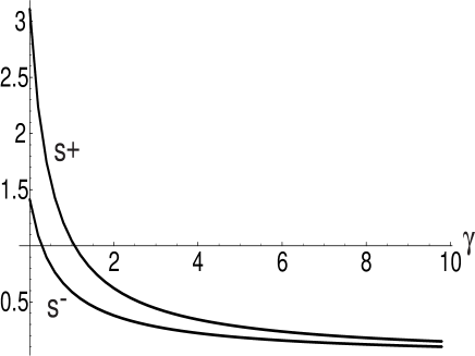
Figure 6: Dependence of velocities $s^{+}$ and $s^{-}$ on the saturation parameter $\gamma$ for fixed values of the intensities at two sides of the dispersive shock: $\rho^{-}=2$ and $\rho^{+}=1$.

Again for small $\gamma$ we can find the correction to Eq. (95) in an explicit form. If we denote $\widetilde{\alpha}=\widetilde{\alpha}_{0}+\widetilde{\alpha}_{1}$, where $\widetilde{\alpha}_{0}$ is given by Eq. (94), then $\widetilde{\alpha}_{1}$ satisfies the equation

$$\frac{d\widetilde{\alpha}_{1}}{d\overline{\rho}}=-\frac{\widetilde{\alpha}_{1}}{2\overline{\rho}}+\frac{8/\sqrt{\overline{\rho}}-6}{4/\sqrt{\rho}-1}\frac{\gamma}{\sqrt{\overline{\rho}}},\qquad\widetilde{\alpha}_{1}(1)=0,$$ (97)

which is readily integrated to give

$$\widetilde{\alpha}_{1}(\rho^{-})=\frac{2\gamma}{\sqrt{\rho^{-}}}\left\{\rho^{-}-1+64\left[\ln\frac{4-\sqrt{\rho^{-}}}{3}+\frac{\sqrt{\rho^{-}}-1}{4}+\frac{\rho^{-}-1}{32}\right]\right\}\,,$$ (98)

and hence

$$s^{-}=\sqrt{\rho^{-}}(1+\widetilde{\alpha}_{1}(\rho^{-}))-\left[\frac{2}{3}(\rho^{-}\sqrt{\rho^{-}}-1)+\rho^{-}(2-\sqrt{\rho^{-}})\right]\gamma.$$ (99)

It is worth noticing that this perturbation approach breaks down for $\rho^{-}\geq 16$ because of logarithmic divergence in Eq. (98) as $\rho^{-}\to 16-0$. The velocities of the dispersive shock edges as functions of the saturation parameter $\gamma$ are shown in Fig 6. As we see, the presence of even small values of the saturation parameters $\gamma$ change the expansion velocities considerably compared with the NLS case $\gamma=0$ because the saturation effects diminish the effective nonlinearity which forces the intensive light beam to expand.

III.3.3 Characteristic velocity ordering

From general point of view, it is important to note that a simple-wave dispersive shock considered above is subject to the conditions similar to “entropy” conditions in viscous shocks theory el ; ekt . Basically, these conditions require that the number of independent parameters characterizing the modulation solution for the dispersive shock must be equal to the number of characteristics families transferring initial data from the $x$ axis into the dispersive shock region in the $(x,t)$ plane. For the photorefractive dispersive shock we have four parameters characterizing the initial step (12) and one algebraic restriction due to the simple-wave transition condition (30). Thus, the number of independent parameters is three. Then, analysis of the characteristic directions at the edges of the dispersive shock waves leads to the following inequalities establishing the ordering between the velocities of the dispersive shock edges and the characteristic velocities (17) of the dispersionless system :

$$V^{-}_{-}<s^{-}<V^{-}_{+},\quad V^{+}_{+}<s^{+},\quad s^{+}>s^{-},$$ (100)

where subscripts correspond to definitions (17) and superscripts to two edges of the dispersive shock with constant values of $\rho^{\pm}$ and $u^{\pm}$. Inequalities (100) provide consistency of the above analytical construction for the derivation of the dispersive shock edges, which heavily relies on the properties of characteristics. We have checked that inequalities (100) are satisfied for a wide range of parameters. As an illustration, we present in Fig. 7 the plots of the characteristic speeds in the simple-wave photorefractive dispersive shock for $\gamma=0.2$ as functions of the intensity jump across the shock. One can see that the ordering (100) is satisfied.

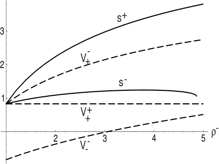
Figure 7: Ordering of the characteristic velocities in the system satisfies inequalities (100).

III.3.4 Vacuum point

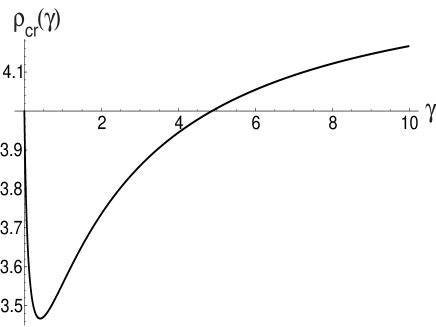
Figure 8: Dependence of the critical intensity $\rho^{-}$ at the trailing edge of the dispersive shock on the saturation parameter $\gamma$ for fixed value of the intensity $\rho^{+}=1$ at the leading edge.

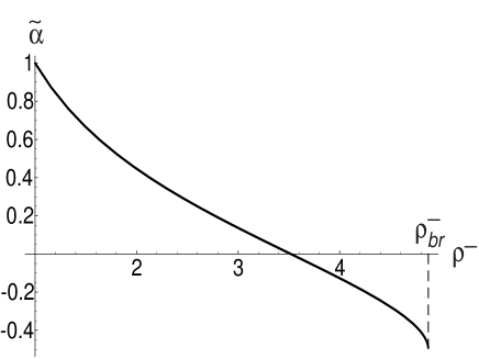
Figure 9: Dependence of the variable $\widetilde{\alpha}$ on the intensity $\rho^{-}$ at the trailing edge of the dispersive shock for fixed value of the intensity $\rho^{+}=1$ at the leading edge at $\gamma=0.2$; the “termination” point corresponds to the intensity $\rho^{-}_{br}=4.873$ where analytical theory loses its applicability.

We now investigate dependence of the main properties of the dispersive shock wave on the value of the intensity jump across the shock, which is equal to the value $\rho^{-}$ at the trailing edge as the value $\rho^{+}=1$ at the leading edge is fixed (of course, we assume $u^{+}=0$ and $u^{-}$ given by Eq. (28)).

It is clear already from the simplest case $\gamma=0$ that there is a possibility for the value $\rho_{m}$ at the minimum of the trailing dark soliton to become zero (or, which is the same, $a=\rho^{-}$) for a certain value of the initial jump $\rho^{-}$. Then it follows from (96) that this happens at $\rho^{-}=4$. This gives rise to a vacuum point with $\rho=0$ at the trailing edge of the dispersive shock eggk95 . When the initial step $\rho^{-}>4$, the vacuum point occurs at some $x_{v}$ inside the dispersive shock zone, $x^{-}<x_{v}<x^{+}$, and the typical profile of the shock changes (see eggk95 ). The appearance of the vacuum point in the dispersive shock is manifested by the singularity in the profile of $u$ at $x=x_{v}$ but the “momentum” $\rho u$ remains finite.

For the photorefractive case, when $\gamma\neq 0$, the critical value of $\rho^{-}=\rho^{-}_{cr}$ corresponding to the appearance of the vacuum point at the trailing edge of the dispersive shock can be found by putting $\rho^{-}=a$ in (92) which immediately yields the equation for $\rho^{-}_{cr}$

$$\widetilde{\alpha}(\rho^{-}_{cr})=0,$$ (101)

where $\tilde{\alpha}(\rho)$ is the solution of the ordinary differential equation (89). The dependence $\rho^{-}_{cr}(\gamma)$ is shown in Fig. 8. Comparison of Eq. (91) with Eq. (28) shows that at the critical point $\rho^{-}=\rho_{cr}^{-}$ we have $s^{-}=u^{-}$, that is the trailing soliton is at rest in the reference frame of the intermediate constant state in the decay of an initial discontinuity (12) (see Section III.A).

The dependence of $\widetilde{\alpha}$ on $\rho^{-}$ is shown in Fig. 9. One should note that the change of sign of $\widetilde{\alpha}$ at $\rho^{-}=\rho_{cr}$ does not constitute nonphysical behaviour even though $\widetilde{\alpha}$ as defined by (88) is a positive value. In fact, for $\rho^{-}>\rho_{cr}$, the velocity $u$ changes its sign at $x=x_{v}$ so that the trailing edge of such a “supercritical” dispersive shock wave propagates to the left relative to the vacuum point. To incorporate this change, one should use another branch in the linear dispersion relation (13) which leads to the change of the sign in the definition of $\widetilde{\alpha}$. As a result, the consistent change of signs in (81) and (89) leads to the same result for the trailing edge speed $s^{-}$ defined by (99).

One can also see from (89) that a singularity in the behaviour of $\widetilde{\alpha}(\rho^{-})$ is expected at some “termination point” $\rho^{-}=\rho^{-}_{br}$ satisfying $2\alpha(\rho^{-})+1=0$ for $\gamma\neq 0$. For $\gamma=0.2$ the value $\rho^{-}_{br}\approx 4.873$. This singularity has also its counterpart in the perturbation theory represented by Eq. (98). The described pathology in the modulation solution for $\rho^{-}\geq\rho^{-}_{br}$, however, is not confirmed by the direct numerical solutions (see Section IV below) and does not seem to have physical sense. One of the explanations of such a discrepancy is that for large values of $\rho^{-}$ the accepted assumption of applicability of the single-phase modulation theory can fail. Indeed, the developed theory is based on the supposition that solutions of our non-integrable photo-refractive system (11) behave qualitatively similar to their counterparts in the integrable NLS equation case so that the dispersive shock wave can be described with high accuracy by the single-phase modulated solution. However, such a supposition can fail in the regions where a drastic change of the behavior of a modulated wave takes place. Just this situation occurs in the vicinity of the vacuum point, at which the profile of $u(x)$ has a singularity. So one can expect some discrepancy between predictions of the modulation theory and exact numerical solutions for the dispersive shock waves with $\rho^{-}$ sufficiently close to or grater than $\rho_{cr}$. As a rough estimate for $\rho^{-}_{cr}$ one can use the value $\rho^{-}_{cr}=4$ obtained for the integrable NLS equation. Since, by definition, $\widetilde{\alpha}(\rho^{-}_{br})=-1/2<0$ for all $\gamma>0$, on can conclude that one always has $\rho^{-}_{br}>\rho^{-}_{cr}$ so the predictions of the developed modulation theory can become unreliable for such large intensity jumps across the dispersive shock.

III.4 Number of solitons generated from a localized initial pulse

Now we consider an asymptotic evolution of a large-scale decaying initial disturbance

$$\rho(x,0)=\rho_{0}(x)\leq 1,\quad u(x,0)=u_{0}(x);\qquad\rho_{0}(x)\to 1\,,\ \ u_{0}(x)\to 0\quad\hbox{as}\quad|x|\to\infty,$$ (102)

so that the typical spatial scale of this disturbance $L\gg 1$. As the numerical simulations for the GNLS equation show, such an initial “well” generally decays as $z\to\infty$ into two groups of dark solitons propagating in opposite directions, which is consistent with the “two-wave” nature of the GNLS equation. For $\gamma=0$ the dynamics is described by the integrable NLS equation and the soliton parameters are found from the generalized Bohr-Sommerfeld rule kku . In the present non-integrable case of the GNLS equation (11) these parameters can be obtained by an extension of the modulation method of obtaining the parameters of the dispersive shock wave for the case when the initial distribution corresponds to the simple wave solution of the dispersionless equations, that is one of the Riemann invariants (15) is supposed to be constant. This extension has been developed in egs in the context of fully nonlinear shallow-water waves and we shall use it here to derive the formula for the total number of solitons resulting from the initial disturbance (102). First, we assume that for the large-scale initial data (102) one can neglect the contribution of the radiation into the asymptotic as $z\to\infty$ solution, which implies that the whole initial disturbance eventually transforms into solitons (this is known to be the case for the integrable NLS equation and is also confirmed by our numerical simulations for the GNLS equation). Next, we notice that this transformation into solitons occurs via an intermediate stage of the dispersive shock wave formation so we can apply the general modulation theory to its description and then to make some inferences pertaining to the eventual soliton train state as $z\to\infty$.

For definiteness, we consider here the right-propagating dispersive shock wave forming from the profile (102) satisfying an additional simple-wave restriction (28)

$$u_{0}(x)=\frac{2}{\sqrt{\gamma}}(\arctan\sqrt{\gamma\rho_{0}(x)}-\arctan\sqrt{\gamma})\,.$$ (103)

We consider the wave number conservation law (54), which is one of the modulation equations describing the dispersive shock wave. For the considered case with decaying at infinity initial profile (102) we have $k\to 0$ as $|x|\to\infty$ and, therefore, equation (54) implies conservation of the total number of waves,

$$N\cong\frac{1}{2\pi}\int^{+\infty}_{-\infty}kdx=\hbox{constant}.$$ (104)

We use an approximate equality sign here due to asymptotic character of the modulation theory which inherently cannot predict an integer $N$ exactly. In the Whitham description of the dispersive shock wave, the $x$-axis is subdivided, after the wave breaking at $z>z_{b}$, into three regions described in Section III.C :

$$-\infty<x<x^{-}(z),\quad x^{-}(z)\leq x\leq x^{+}(z),\quad x^{+}(z)<x<\infty\,,$$ (105)

where $x^{\pm}(z)$ are the boundaries of the dispersive shock wave. Generally, these boundaries are not straight lines as in the case of the decay of the initial step-like pulse considered above but their nature as characteristics of the modulation system remains unchanged. In view of (105), the integral in (104) can be expressed as a sum of three integrals,

$$N\cong\frac{1}{2\pi}\left\{\int^{x^{-}(z)}_{-\infty}k(x,z)dx+\int^{x^{+}(z)}_{x^{-}(z)}k(x,z)dx+\int_{x^{+}(z)}^{\infty}k(x,z)dx\right\}.$$ (106)

To apply formula (106) we need first to define the wavenumber $k$ outside the dispersive shock wave as it has been actually defined so far only within the nonlinear modulated wave region $[x^{-}(z),x^{+}(z)]$. The extended definition of $k$ should be consistent with the matching conditions (50), (51) for all $z$.

We know that at the soliton edge $x^{-}(z)$ of the Whitham zone we have $k(x^{-}(z),z)=0$, so we can safely put $k(x,z)=0$ in the region $x<x^{-}(z)$ and, hence, the first integral vanishes. At the same time, the value of $k$ is not explicitly prescribed at the leading edge $x^{+}(z)$ by the boundary condition (50) but is rather determined as a function of $\rho$ due to the fact that the leading edge is a characteristic of the modulation system — see Section III.C. The dependence $k^{+}(\rho)$ is determined then by the ordinary differential equation (63) (we note that the simple-wave transition condition (28) is already embedded in (63) and is consistent with the initial conditions (103)). This ordinary differential equation should be, again, solved with the initial condition $k(\rho^{-})=0$, and now $\rho^{-}=\rho_{b}\cong 1$ where we have taken into account that for large pulse (102) the wave breaking occurs close to the background intensity, $\rho_{b}\cong 1$. Thus, we get the characteristic integral $k=k^{+}(\rho)$ along the leading edge. The intensity $\rho(x,z)$ in the downstream region $x>x^{+}(z)$ satisfies the simple-wave dispersionless equation

$$\rho_{z}+V_{+}(\rho)\rho_{x}=0$$ (107)

with the initial condition $\rho(x,0)=\rho_{0}(x)$, i.e. the solution is given implicitly by $\rho=\rho_{0}(x-V_{+}(\rho)z)$. Therefore, to be consistent with the boundary values of $k$ prescribed by the characteristic integral of the modulation equations, we have to define the wave number downstream the dispersive shock wave as $k^{+}(\rho(x,z))$, where $\rho(x,z)$ is the aforementioned simple-wave solution. Then, at $z=0$ we get an effective initial distribution of $k$ in terms of the initial data for $\rho$ given by (102):

$$k(x,0)=k^{+}(\rho_{0}(x))\,$$ (108)

for $x\geq x_{b}$, where $x_{b}$ is the coordinate of the breaking point; obviously $x_{b}=x^{-}(z_{b})=x^{+}(z_{b})$. Note that this definition is also consistent with our definition $k\equiv 0$ upstream of the dispersive shock wave, since $k^{+}(1)=0$. Thus, (108) describes initial data for the wave number for all $x$. The function $k(x,0)$ can be interpreted as the wave number distribution for a “virtual” linear modulated wave which accompanies the initial hydrodynamic distributions $(\rho(x,0)$, $u(x,0)$ and transforms, after the wave breaking, into the dispersive shock and, eventually, into a train of solitons.

Now, we consider (106) for $z=0$ and notice that, since the second integral disappears for $z<z_{b}$, $z_{b}>0$ (there is no dispersive shock before the breaking point formation so we put $x^{+}(z)=x^{-}(z)$ for $z\leq z_{b}$), this expression reduces to

$$N\cong\int_{-\infty}^{\infty}k(x,0)dx=\int_{-\infty}^{\infty}k^{+}(\rho_{0}(x))dx.$$ (109)

As was shown in Section III.C, it is convenient to introduce an auxiliary function $\alpha(\rho)$ instead of $k^{+}(\rho)$ according to (64) so that

$$k^{+}=2\frac{\sqrt{\rho(\alpha^{2}-1)}}{1+\gamma\rho}.$$ (110)

Then $\alpha(\rho)$ satisfies the ordinary differential equation (65) with the initial condition $\alpha(1)=1$. As a result, the number of solitons as $z\to\infty$ is determined by the formula

$$N\cong\frac{1}{2\pi}\int^{+\infty}_{-\infty}k(x,0)dx=\frac{1}{\pi}\int^{+\infty}_{-\infty}\frac{\sqrt{\rho_{0}(x)(\alpha_{0}^{2}(x)-1)}}{1+\gamma\rho_{0}(x)}dx,$$ (111)

where $\alpha_{0}(x)=\alpha(\rho_{0}(x))$.

When $\gamma=0$, the solution $\alpha(\rho)$ of (65) is given by (70) and assumes here the form

$$\alpha=\frac{2}{\sqrt{\rho}}-1\ \qquad\hbox{for}\quad\gamma=0.$$ (112)

Then, for the total number of solitons we have from (111)

$$N\cong\frac{1}{\pi}\int^{+\infty}_{-\infty}\sqrt{(2-\sqrt{\rho_{0}(x)})^{2}-\rho_{0}(x)}=\frac{2}{\pi}\int^{+\infty}_{-\infty}\sqrt{1-\rho_{0}^{1/2}}dx\,\qquad\hbox{for}\quad\gamma=0,$$ (113)

which agrees with the “simple-wave” reduction of the semi-classical quantization results for the defocusing NLS equation obtained in kku .

IV Numerical simulations of nonlinear waves in photorefractive media

In this Section, we compare the analytical predictions of the preceding Sections with the results of direct numerical simulation of the formation of dispersive shock waves in photorefractive equation (4).

First, we have studied numerically evolution of the step-like pulse. The corresponding results are shown in Fig. 10. As we see, all the parameters (velocities of the edges of the rarefaction wave and the dispersive shock, intensity of the intermediate state) are in a good agreement with the analytical predictions of Section III.A.

Figure 10: Evolution of the initial step-like pulse with $\rho_{0}=5$ and $\rho=1$ for the case of $\gamma=0.1$. The general structure confirms formation of a rarefaction wave, a dispersive shock and an intermediate constant state in between. Intensity $\rho^{-}=2.466$ calculated according to Eq. (27) coincides with the numerical result for the intensity of the intermediate state. Coordinates of the edges of the rarefaction wave at $t=32$ calculated analytically are equal to $x_{1}^{-}=-47.7$, $x_{1}^{+}=-9.02$ for the rarefaction wave and $x_{2}^{-}=42.57$, $x_{2}^{+}=99.52$. One can see that they agree quite well with numerical results. Small-amplitude waves generated at around $x=-50$ correspond to the linear dispersive “resolution” of the weak discontinuity occurring at the trailing edge of the rarefaction wave.

We have constructed the dependence of $\rho^{-}$ and $u^{-}$ on the saturation parameter $\gamma$ using the results of the numerical simulations. The results shown in Fig. 11 agree very well with the analytical predictions based on the “simple-wave” jump condition (30) which is applicable for not too large values of $\rho^{-}$ ($\lesssim 4$) such that the vacuum point is not formed.

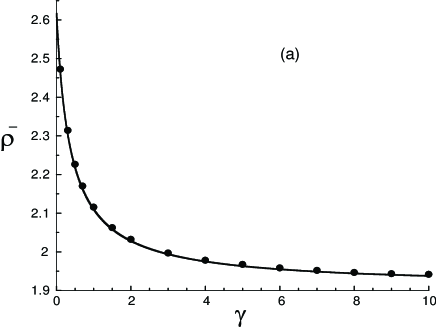
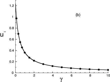
Figure 11: Dependence of intermediate values (solid lines) of intensity (a) and transverse wave vector (b) on the saturation parameter $\gamma$ for fixed values of the initial discontinuity parameters: $\rho_{0}=5$, $u_{0}=0$ for $x<0$ and $\rho^{+}=1$, $u^{+}=0$ for $x>0$ at $z=0$. Numerically calculated values are shown by crosses.

In Fig. 12 we show the dependence of the edge “velocities” $s^{\pm}$ on the intermediate intensity $\rho^{-}$ (with $u^{-}$ calculated according to “simple-wave” jump condition (28)). As we see, a good agreement is observed for $\rho^{-}<4$.

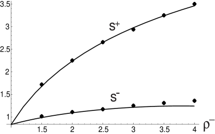
Figure 12: Dependence of $s^{\pm}$ on $\rho^{-}$ (with $u^{-}$ calculated according to (28)); $\gamma=0.2$. Solid lines correspond to analytical formulae (68) and (91), and dots correspond to results of numeric simulations.

However, as $\rho^{-}$ increases with growth of $\rho_{0}$ and becomes greater than $\rho^{-}_{cr}\simeq 4$, Eq. (28) no longer yields the values of $u^{-}$ compatible with the prescribed value of $\rho^{-}$ so that only a single right-propagating dispersive shock is generated; this is illustrated by Fig. 13, where a new “intermediate” region of constant flow is seen to be formed which matches with the dispersive shock propagating to the right, while another dispersive shock is apparently forming to the left of this new constant state providing matching with $\rho_{0}$.

Figure 13: Dispersive shock evolving from the step-like pulse with $\rho^{-}$ and $u^{-}$ related by the “simple-wave” jump condition for large value of $\rho^{-}=10$ much greater than $\rho^{-}=4$. Occurrence of a vacuum point in the region between $x=100$ and $x=150$ is clearly seen. A new intermediate constant state is formed in the region behind the dispersive shock showing that the simple-wave jump condition (28) does not prevent anymore the formation of the second wave for large values of $\rho^{-}$.

Surprisingly, we have found that the large-amplitude dispersive shock wave transition between the new intermediate constant state and $\rho=1$ now satisfies a classical shock jump condition which follows from the balance of “mass” and “momentum” across the shock as it takes place in classical dissipative shocks. Using the dispersionless equations (14) represented in a conservative form we find that formal shock jump conditions yield the dependence

$$u^{-}=\frac{\sqrt{2}(\rho^{-}-1)}{\sqrt{(\rho^{-}+1)(1+\gamma\rho)(1+\gamma)}}\,.$$ (114)

We have checked that dependence (114) is indeed satisfied very well for $\rho^{-}>4$. The physical mechanism supporting the appearance of the classical shock conditions in a dissipationless system such as (11) is not quite clear at the moment. We note that similar effect of appearance of the classical shock jump condition across the expanding dispersive shock have been recently observed in egs2006 for large-amplitude shallow-water undular bores modeled by the Green-Naghdi system, which is also not integrable by the IST. At the same time, it is known very well that for the dispersive shocks described by the integrable NLS equation, the simple-wave jump condition is satisfied exactly for all values of initial density jump – this follows from the full modulation solution (see eggk95 , kodama , hoefer ) and is also confirmed by our numerical simulations. So it is possible that the described phenomenon of the appearance of the classical shock conditions constitutes a specific manifestation of nonintegrability in dispersive dissipationless systems which is yet to be explored.

Next, we have compared the analytical predictions of subsection III.D for number of dark solitons generated from a hole-like disturbance with numerical simulations. We took the initial distribution of intensity

$$\rho_{0}(x)=\left(1-\frac{1}{\cosh(0.2x)}\right)^{2}$$ (115)

and the initial distribution of transverse wave number was calculated according to the equation (103). Evolution of such a pulse according to the photorefractive equation with $\gamma=0.2$ is illustrated by Fig. 14 where the profile of intensity is shown at $z=100$.

Figure 14: Profile of intensity at $z=100$ evolved from the initial pulse (115) (dashed line) with initial profile of $u(x)$ calculated according to (103).

As we see, this pulse, after the wave breaking and formation of a dispersive shock, evolves eventually into a number of dark solitons. We note that the appearance of several solitons propagating to the left does not contradict to the unidirectional restriction guaranteed by the simple-wave initial conditions (115), (103) – these left-propagating solitons occur due to relatively high amplitude of the initial disturbance (115), which leads to the appearance of the vacuum point at the intermediate stage of the dispersive shock wave and, therefore, to the formation of some number of left-propagating solitons – see Section III.C. The total number of created solitons calculated by means of the modulation formula (111) as a function of the saturation parameter $\gamma$ is shown by solid line in Fig. 15 and the corresponding results of numerical simulations are indicated by dots. Taking into account the asymptotic nature of the developed analytical theory for this integer-valued function, and the fact that considered initial data (115) produce a vacuum point (i.e. at some stage of the dispersive shock development the “instantaneous” initial jump $\rho^{-}>\rho^{-}_{cr}$), the agreement can be considered as quite good.

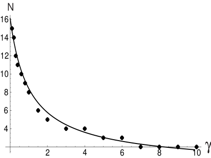
Figure 15: Number of solitons $N$ as a function of $\gamma$; solid line represents analytical dependence (111) and dots correspond to numerical simulations.

In Refs. hoefer ; fleischer the theory of dispersive shocks, evolving from a step-like pulse according to the NLS equation (5) ($\gamma=0$) was used for qualitative explanation of dispersive shocks with other geometries in concrete physical situations (see also kgk04 where the NLS theory of the wave breaking was also used for description of dispersive shocks in Bose-Einstein condensates). In a similar way, the developed here theory of dispersive shocks in photorefractive media can be used for the description of experiments on generation of optical shocks. Such experiments were described in french ; fleischer and here we present some results based on the numerical solutions of the photorefractive equation (4) with the initial conditions similar to the initial light distributions in the mentioned experimental works (similar results of numerical simulation were presented in fleischer ).

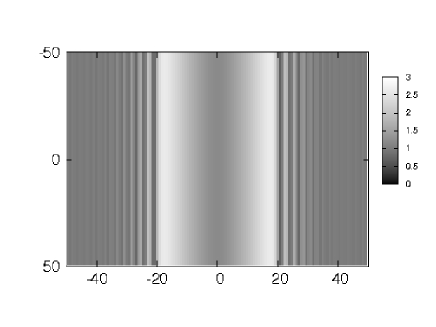
Figure 16: Density plot of the output intensity evolved from a strip-like initial distribution.

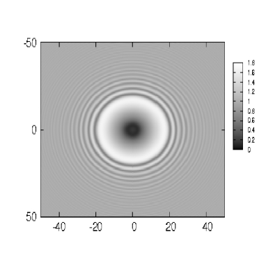
Figure 17: Density plot of the output intensity evolved from a circle initial distribution.

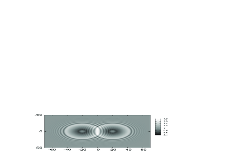
Figure 18: Interaction of two circular dispersive shocks.

In fleischer the distribution of output intensities are presented for initial distributions in the form of a strip, a circle, and two separated circles. We have performed numerical simulations with similar initial conditions. In Fig. 16 we present a density plot of the output intensity evolved, according to the photorefractive equation with $\gamma=0.1$, from the strip-like initial distribution given by the formula

$$\rho(x)=\left\{\begin{array}[]{ll}1+5(1-x^{2}/25)^{0.2}&\text{for}\quad|x|<5,\\ 1&\text{for}\quad|x|>5,\end{array}\right.$$ (116)

which approximates with a good enough accuracy the constant values of intensities inside the strip and outside it. Similar density plot for the circle initial distribution is shown in Fig. 17.

As we see, in both cases the initial “hump” breaks with formation of dispersive shocks—in the strip-like geometry we get two shocks propagating in opposite directions and in circular geometry we have a ring-like dispersive shock expanding in radial direction.

In Fig. 18 an interaction of two circular dispersive shock waves is shown. It is remarkable that even in this two-dimensional nonintegrable photorefractive case, the nonlinear dispersive shock waves interact apparently elastically, without production of other waves in the region of their overlap. It is this kind of picture that is expected in the system with $\gamma=0$ described by the integrable NLS equation where the interaction of two dispersive shocks leads to the formation of a two-phase modulated wave region described by the corresponding multiphased-averaged modulation system bk . While the analytical description of multiphase nonlinear waves in photorefractive equation (11) is not available, the qualitative similarity between the solution behaviour for the nonintegrable photorefractive equation and for the NLS equation for moderate values of initial amplitudes can be considered as a confirmation of robustness of the modulated travelling wave ansatz in the description of dispersive shock waves in nonintegrable systems, at least for some reasonable range of initial amplitudes.

V Conclusion

In this paper, we have developed the theory of formation of dispersive shocks in propagation of intensive light beams in photorefractive optical systems. The theory is based on Whitham’s modulation approach in which a dispersive shock is described as a modulated nonlinear periodic wave and slow evolution along the propagation axis is governed by the averaged modulation equation. In spite of the absence of complete integrability of the equation describing propagation of light beams in photorefractive media, the main characteristic parameters of shocks can be determined by means of the approach developed in el –ekt and based on the study of reductions of Whitham equations for the wave regimes realized at the boundaries of the dispersive shock. In particular, “velocities” of the dispersive shock edges are found as functions of the jump of intensity across the shock as well as amplitude of the soliton at the rear edge of the shock. The number of solitons produced from a finite initial disturbance is also determined analytically for initial distributions related by a so-called simple wave condition. The analytical theory agrees very well with numerical simulations as long as there is no vacuum point in the shock. Appearance of a vacuum point leads to the formation of a singularity in a “transverse” wavevector distribution and such a drastic change in the wave behavior cannot be traced by the developed approach. However, this situation occurs at very high input intensities of a light beam so that for practical purposes the developed theory provides accurate enough approximation.

Although the theory is essentially one-dimensional (i.e. with one transverse space coordinate) it can give qualitative explanation of experiments with other geometries, which is illustrated by the results of numerical simulations.

Acknowledgments

This work was supported by FAPESP (Brazil) and EPSRC (UK). AMK thanks also RFBR (grant 05-02-17351) for partial support.

References

- (1) Yu.S. Kivshar and G.P. Agraval, Optical solitons. From Fibers to Photonic Crystals, (Academic Press, Amsterdam, 2003).
- (2) W. Królikowski and B. Luther-Davies, IEEE J. Quantum Electronics, 39, 3 (2003).
- (3) G.B. Whitham, Linear and Nonlinear Waves, (Wiley-Interscience, 1974).
- (4) B. Benjamin and M.J. Lighthill, Proc. Roy. Soc. London, A 224, 448 (1954).
- (5) M. Khan, S. Ghosh, S. Sarkar, and M.R. Gupta, Phys. Scr. T 116, 5356 (2005).
- (6) M.A. Hoefer, M.J. Ablowitz, I. Coddington, E.A. Cornell, P. Engels, and V. Schweikhard, Phys. Rev. A 74, 023623 (2006).
- (7) G. Couton, H. Mailotte, and M. Chauvet, J. Opt. B: Quantum Semicl Opt., 6, S223 (2004).
- (8) W. Wan, S. Jia, and J.W. Fleischer, Nature Physics, 3, 46 (2007).
- (9) G. Rowlands and E. Infeld, Nonlinear Waves, Solitons, and Chaos, 2nd ed. Cambridge, England: Cambridge University Press (2000).
- (10) A.M. Kamchatnov, Nonlinear Periodic Waves and Their Modulations (Singapore, World Scientific, 2000).
- (11) M.G. Forest and J. Lee, in Oscillation Theory, Computation, and Methods of Compensed Compactness, edited by C. Dafermos et al, (Springer, New York, 1986), Vol. 2, pp. 35–69.
- (12) M.V. Pavlov, Theor. Math. Phys., 71, 584 (1987).
- (13) A.V. Gurevich and A.L. Krylov, ZhETF 92, 1684 (1987).
- (14) G.A. El, V.V. Geogjaev, A.V. Gurevich, and A.L. Krylov, Physica D 87, 186 (1995).
- (15) G.A. El and A.L. Krylov, Phys. Lett. A (1995).
- (16) S. Jin, C.D. Levermore, D.W. McLaughlin, Comm. Pure Appl. Math., 52, 613 (1999).
- (17) F.-R. Tian and J. Ye, Comm. Pure Appl. Math. 52, 655 (1999).
- (18) A.M. Kamchatnov, R.A. Kraenkel, B.A. Umarov, Phys. Rev. E 66, 036609 (2002).
- (19) G. Biondini and Y. Kodama, J. Nonlinear Sci., 16 435 (2006).
- (20) Y. Kodama, SIAM J. Appl. Math., 59, 2162 (1999).
- (21) A.M. Kamchatnov, A. Gammal, and R.A. Kraenkel, Phys. Rev. A 69, 063605 (2004).
- (22) G.A. El, Chaos, 15, 037103 (2005).
- (23) A.V. Tyurina and G.A. El, JETP, 88, 615 (1999).
- (24) G.A. El, V.V. Khodorovskii, A.V. Tyurina, Physica D 206, 232 (2005).
- (25) G. Duree, M. Morin, G. Salamo, M. Segev, B. Crosignani, P. Di Porto, E. Sharp, and A. Yariv, Phys. Rev. Lett. 74, 1978 (1995).
- (26) L.D Landau and E.M. Lifshitz, Fluid Mechanics, Pergamon, Oxford, (1987).
- (27) A.V. Gurevich and L.P. Pitaevskii, Sov. Phys. JETP 38, 291 (1974).
- (28) A.V. Gurevich and A.P. Meshcherkin, Sov. Phys. JETP, 60, 732 (1984).
- (29) C. Hou, Y. Pei, Z. Zhou, and X. Sun, Phys. Rev. A 71, 053817 (2005).
- (30) R. Courant and D. Hilbert, Methods of Mathematical Physics, vol II, Wiley-Interscience, New York, (1962).
- (31) S.A. Darmanyan, A.M. Kamchatnov, and S.A. Neviére, JETP 96, 876 (2003).
- (32) R. Grimshaw, Proc. Roy. Soc. 368A, 359 (1979).
- (33) G.A. El, R.H.J. Grimshaw and N.F. Smyth, Semi-classical distributions of solitary waves in fully nonlinear shallow-water theory, to be published.
- (34) G.A. El, R.H.J. Grimshaw and N.F. Smyth, Phys. Fluids 18, 027104 (2006).