Block scaling in the directed percolation universality class

Abstract

The universal behaviour of the directed percolation universality class is well understood, both the critical scaling as well as finite size scaling. This article focuses on the block (finite size) scaling of the order parameter and its fluctuations, considering (sub-)blocks of linear size $l$ in systems of linear size $L$. The scaling depends on the choice of the ensemble, as only the conditional ensemble produces the block-scaling behaviour as established in equilibrium critical phenomena. The dependence on the ensemble can be understood by an additional symmetry present in the unconditional ensemble. The unconventional scaling found in the unconditional ensemble is a reminder of the possibility that scaling functions themselves have a power-law dependence on their arguments.

1 Introduction

The directed percolation (DP) universality class comprises a huge number of non-equilibrium critical phenomena. Janssen and Grassberger [1, 2] famously conjectured more than 25 years ago that under very general circumstances, all models with a unique absorbing state belong to the DP universality class. While this conjecture has been confirmed numerically many times, evidence for the presence of the DP universality class in natural systems is still very scarce [3] (but see [4]).

One problem, when probing field data for the presence of DP is that field data is more readily obtained in a single measurement rather than as a time series. However, the statistical features to be identified require an entire ensemble of realisations of the process in question. Instead of using a time series, one can resort to sub-sampling, i.e. splitting a large sample of size $L^{d}$ into $(L/l)^{d}$ small ones of size $l^{d}$. For example, a population pattern obtained by measuring the spatial distribution of species could be split into several distinct blocks and their mutual correlations analysed.

The question how the order parameter of an equilibrium system at the critical point changes with the block size it is averaged over, has been studied in great detail by Binder [5]. In the present work, a corresponding analysis is applied to models belonging to the DP universality class, more specifically to the contact process and to directed percolation itself from the point of view of absorbing state (AS) phase transitions. It turns out that the block averaged order parameter needs to be defined very carefully in order to reproduce standard finite size scaling. In the following, I will present numerical evidence and theoretical arguments that block finite size scaling (FSS) in DP can be very different from what is expected from equilibrium critical phenomena, depending on the choice of the ensemble. This observation can be readily applied to the analysis of field data, and will be illustrated using surrogate data.

2 Method

The order parameter of an absorbing state phase transition is the activity $\rho$, which, in lattice models, is the density of active sites. The activity vanishes as soon as the system hits the absorbing state, from where it cannot escape. In a finite system, the absorbing state is reached with finite probability from anywhere in phase space, so that every (finite) system eventually becomes inactive, $\lim_{t\to\infty}\rho(t)=0$, where $t$ measures the time in the model. However, the order parameter $\rho$ signals a phase transition in a temperature-like tuning parameter $p$, dividing the parameter space into a region where the decay of the activity $\rho$ is exponentially fast in time, from a region where for sufficiently large systems it is practically impossible to observe $\rho=0$.

At least two (seemingly) different methods have been devised to overcome the problem that strictly $\lim_{t\to\infty}\rho(t)=0$ and to obtain the phase transition even in finite systems: One either introduces an external field which induces activity in the system [6] and analyses the model in the limit of arbitrarily small fields, or one considers the quasi-stationary state [7]. In this latter approach, after initialising and discarding a transient, all averages are taken conditional to activity. The activity entering the observables therefore never vanishes and the order parameter is always non-zero, rendering for example moment ratios well defined. One can show that both methods produce asymptotically equivalent scaling results [8]. In the present article, the quasi-stationary state was used to produce individual samples.

Above the critical point $p_{c}$, i.e. for $p>p_{c}$, the ensemble average of the activity $\rho$ in the thermodynamic limit picks up as a power-law $\left\langle\rho\right\rangle=A(p-p_{c})^{\beta}$, where $A$ is the amplitude, $p_{c}$ is the critical value of the tuning parameter and $\beta$ is a universal critical index. Similarly, fluctuations of the order parameter scale as $\sigma^{2}\left(\rho\right)\equiv\left\langle\rho^{2}\right\rangle-\left\langle\rho\right\rangle^{2}=B_{\pm}L^{-d}|p-p_{c}|^{-\gamma}$, where $B_{+}$ and $B_{-}$ are the amplitudes above and below the transition respectively, $L$ is the linear extent of the system, $d$ is its spatial dimension and $\gamma$ is an independent critical exponent. Both these power laws are asymptotes and thus acquire corrections [9] away from the critical point.

Ordinary FSS [10, 11, 12] is observed by tuning $p=p_{c}$ and considering the behaviour of the observables as a function of the system size, $\left\langle\rho\right\rangle(L)=A^{\prime}L^{-\beta/\nu_{\perp}}$ and $\sigma^{2}\left(\rho\right)(L)=B^{\prime}L^{-d+\gamma/\nu_{\perp}}$, where $\nu_{\perp}$ is a third critical exponent. These exponents are related by $-d+\gamma/\nu_{\perp}=-2\beta/\nu_{\perp}$ [13], which in equilibrium corresponds to Josephson hyper-scaling together with the Rushbrooke scaling law.

Another kind of FSS can be explored in addition to the ordinary one just described. Instead of considering the entire system, observables are recorded within small blocks of linear extent $l$. To this end, I introduce the observables $\left\langle\rho\right\rangle_{u}(l;L)$ and $\sigma^{2}_{u}\left(\rho\right)(l;L)$, which are first and second cumulants of the activity within those blocks of linear size $l$ in a system of size $L$. The blocks are produced by dividing samples of linear size $L$ generated in the quasi-stationary state into $(L/l)^{d}$ blocks of linear size $l$ each. This length $l$ is conveniently chosen so that it divides $L$. By construction, each sample of size $L^{d}$ contains at least one active site and consequently at least one block of size $l^{d}$ has non-vanishing activity. However, there may be up to $(L/l)^{d}-1$ inactive blocks.

In addition to these observables, I introduce $\left\langle\rho\right\rangle_{c}(l;L)$ and $\sigma^{2}_{c}\left(\rho\right)(l;L)$, which are the first and second cumulant of the activity conditional to activity within the respective block. That means that inactive blocks are discarded when averaging. To distinguish the two ensembles, the former (with cumulants $\left\langle\rho\right\rangle_{u}(l;L)$ and $\sigma^{2}_{u}\left(\rho\right)(l;L)$) will be called “unconditional” (subscript $u$) and the latter (with cumulants $\left\langle\rho\right\rangle_{c}(l;L)$ and $\sigma^{2}_{c}\left(\rho\right)(l;L)$) “conditional” (subscript $c$). One can derive the moments of the unconditional ensemble from the corresponding moments in the conditional ensemble and vice versa by re-weighting, because they differ only by a number of samples with vanishing block-activity which are discarded in the conditional ensemble but not in the unconditional one (see [8] for similar considerations for the overall activity). If the fraction of active blocks averaged over the entire unconditional ensemble is $a(l;L)$, then the $n$th moment of the unconditional ensemble $\left\langle\rho^{n}\right\rangle_{u}$ is related to the $n$th moment of the conditional ensemble $\left\langle\rho^{n}\right\rangle_{c}$ by

$$\left\langle\rho^{n}\right\rangle_{u}(l;L)=a(l;L)\left\langle\rho^{n}\right\rangle_{c}(l;L)$$ (1)

for $n>0$.

More than 25 years ago, block scaling was investigated by Binder [5] for the Ising model, where the order parameter is the magnetisation density $m$ rather than the activity $\rho$. In these systems with a symmetric phase-space, there is no corresponding distinction of active and inactive blocks. Naïvely transferring these results to DP suggests

$$\left\langle\rho\right\rangle_{u,c}(l;L)=C_{u,c}l^{-\beta/\nu_{\perp}}\mathcal{G}_{u,c}(l/L)$$ (2)

in leading order of $L$ and in the limit of $l$ being large compared to a lower cutoff $l_{0}$, i.e. $l\gg l_{0}$. Below this constant threshold $l_{0}$, i.e. $l<l_{0}$, the order parameter deviates from the behaviour predicted by (2). This phenomenon is known and well understood in classical critical phenomena [14, 12]. In the following, data for $l\leq l_{0}$ is not shown; in the two-dimensional contact process and directed percolation $l_{0}$ was estimated to be $l_{0}\approx 8$ and in the one-dimensional contact process $l_{0}\approx 16$.

The dimensionless scaling functions $\mathcal{G}_{u,c}(x)$ in (2) are bounded from above and usually also from below (away from 0) for all $x\in[0,1]$. The scaling function is universal up to a pre-factor, which can always be absorbed into the metric factor $C_{u,c}$. The latter is required for dimensional consistency.

Scaling behaviour similar to (2) is expected to hold for higher order moments and cumulants as well, in particular for the variance of the activity

$$\sigma^{2}_{u,c}\left(\rho\right)(l;L)=D_{u,c}l^{-2\beta/\nu_{\perp}}\mathcal{F}_{u,c}(l/L)\ ,$$ (3)

using the scaling relations cited above. Again, the scaling functions $\mathcal{F}_{u,c}$ are constraint by being bounded from above and (usually) away from zero from below.

So far, I have described what is expected in absorbing state systems as inferred from equilibrium critical phenomena. In the remainder of this article, I will first introduce the non-equilibrium models and the methods used in the numerical simulations for this study. The results for the different observables (activity, its variance and a moment ratio) in the different ensembles (unconditional and conditional) are then discussed in the light of analytical arguments. The article finishes with an application to surrogate data, a discussion of the implications and the wider context of the findings and concludes with a brief summary.

3 Results

Most of the numerics in this work is based on the contact process [15, 13] on a two-dimensional square lattice with periodic boundary conditions, but the same results are found for the one-dimensional contact process as well as for two-dimensional site-directed percolation [16]. In fact, it will be argued that they are general features of the directed percolation universality class, if not of all absorbing state phase transition. In the two-dimensional contact process occupied sites turn empty with extinction rate $1$, while empty sites become occupied with rate $z\lambda$ with $z$ being the fraction of occupied nearest neighbours. The critical value of $\lambda$ has been estimated numerically with great accuracy $\lambda_{c}=1.64877(3)$ [17] (I used $\lambda=1.6488$ in the present study). The time scale is set by the extinction rate. The two-dimensional contact process belongs to the DP universality class which is characterised by exponents $\beta=0.583(3)$, $\gamma=0.297(2)$ and $\nu_{\perp}=0.733(4)$ [18], so that $\beta/\nu_{\perp}=0.795(6)$.

In site-directed percolation in $2+1$ dimensions (BCC lattice) the time evolves discretely [16, 19]. A site is occupied in the following time step with probability $p$ if at least one of its directed neighbours is occupied, otherwise it is empty. The directed neighbours of a site are four sites in the preceding time step: The site itself, its right and upper nearest neighbour and its upper right next nearest neighbour. The critical value of $p$ in this model has been estimated as $p_{c}=0.34457(1)$ [18]. This model belongs to the 2D DP universality class as well.

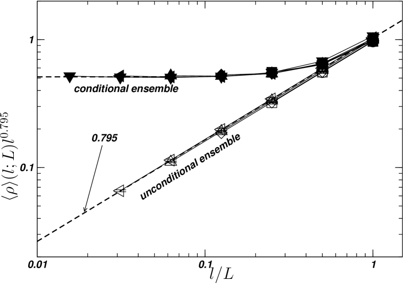
Figure 1: Data collapse of the order parameter measured in the unconditional (open symbols) and the conditional ensemble (filled symbols) for the two-dimensional contact process with system sizes $L=32,64,\ldots,512$ (up to $L=1024$ in the conditional ensemble) and $l=16,32,\ldots,L$ (data points for the same system size obtained from the same samples are connected by lines). The unconditional order parameter collapses trivially (see text) and is shown for illustration purposes only. The sloped dashed line has slope $0.795\approx\beta/\nu_{\perp}$, indicating the power-law behaviour of the scaling function of the unconditional ensemble, $\mathcal{G}_{u}$, defined in (2). The conditional order parameter collapses well under the scaling ansatz (2), plotting $\left\langle\rho\right\rangle_{c}(l;L)l^{\beta/\nu_{\perp}}$ vs. $l/L$. The horizontal dashed line is the likely asymptote of the scaling function $\mathcal{G}_{c}$ in the conditional ensemble.

All measurements are taken at the quasi-stationary state: Starting from random initial configurations with a small but non-vanishing activity, the systems evolve according to the rules described above, until the observables reach a (quasi-)stationary state. For example, in the two-dimensional CP for $L=256$, the first $10^{5}$ updates are discarded as transient. Measurements are taken at constant rate after the transient and enter with the same weight until the system reaches the absorbing state (for $L=256$ the average lifetime was about $4.8\cdot 10^{4}$) or a maximum time is reached ($5\cdot 10^{5}$ for $L=256$). The procedure is repeated until the statistical error is acceptably small; for example $1.42\cdot 10^{8}$ systems of size $L=256$ were started, of which only about $13\%$ survive the transient. Statistical errors were estimated by sub-sampling the ensemble, which copes even with correlated data. In the following, the scaling of the various (block) observables in $l$ and $L$ is analysed.

3.1 Order parameter

The first moment of the activity in the unconditional ensemble, $\left\langle\rho\right\rangle_{u}(l;L)$, does not vary in $l$ at all, because of translational invariance: Every (randomly chosen) site is equally likely to be active and therefore $\left\langle\rho\right\rangle_{u}(l;L)$ is constant in $l$. In order to establish ordinary FSS complying to (2), the scaling function $\mathcal{G}_{u}(x)$ must necessarily be a power-law itself, $\mathcal{G}_{u}(x)=\mathcal{G}_{u}(1)x^{\beta/\nu}$, so that

$$\left\langle\rho\right\rangle_{u}(l;L)=C_{u}\mathcal{G}_{u}(1)L^{-\beta/\nu}$$ (4)

otherwise standard finite size scaling, $\left\langle\rho\right\rangle_{u}(l=L;L)\propto L^{-\beta/\nu}$, would not be recovered for $l=L$, i.e. when a single block covers the entire system. Contrary to what is expected from equilibrium critical phenomena, this scaling function necessarily vanishes at $0$, i.e. $\lim_{x\to 0}\mathcal{G}_{u}(x)=0$. Figure 1 contains a (trivial) data collapse for $\left\langle\rho\right\rangle_{u}(l;L)$ according to (2), namely $\left\langle\rho\right\rangle_{u}(l;L)l^{\beta/\nu_{\perp}}\propto(l/L)^{\beta/\nu_{\perp}}$ as a function of $l/L$ for various system sizes $L$, which illustrates the scaling behaviour.

The conditional order parameter $\left\langle\rho\right\rangle_{c}(l;L)$, on the other hand, does not suffer from this complication. By construction at least one site per patch is active, $\left\langle\rho\right\rangle_{c}(l;L)\geq l^{-d}$, so that $\lim_{L\to\infty}\left\langle\rho\right\rangle_{c}(l;L)\geq l^{-d}$. The latter limit is the thermodynamic limit of a density and its existence is the most basic assumption in statistical mechanics. Provided $l$ is sufficiently large compared to the fixed lower cutoff $l_{0}$, so that (2) applies, the limit implies that $\lim_{x\to 0}\mathcal{G}_{c}(x)>0$, i.e. $\mathcal{G}_{c}(x)$ converges to a non-zero value. This is numerically confirmed by the data collapse of $\left\langle\rho\right\rangle_{c}(l;L)$ in Figure 1.

3.2 Variance of the order parameter

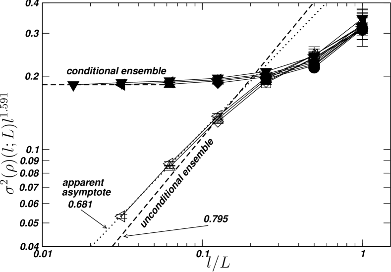
Figure 2: Data collapse of the variance of the order parameter in the unconditional (open symbols) and the conditional ensemble (filled symbols), as in Figure 1. The data is shown in rescaled form, as $\sigma^{2}\left(\rho\right)(l;L)l^{2\beta/\nu_{\perp}}$ vs. $l/L$. Again, the horizontal dashed line is the likely asymptote of the scaling function $\mathcal{F}_{c}$ (see (3)) of the conditional ensemble, while the sloped dashed line has slope $\beta/\nu_{\perp}\approx 0.795$, expected to be the asymptote of the unconditional ensemble. The dotted line (apparent asymptote) with slope $0.681$, however, fits the numerical data very convincingly, indicating that the asymptotic regime has not yet been reached.

The considerations are similar for the second cumulant, $\sigma^{2}_{u,c}\left(\rho\right)(l;L)$. At $l=1$ the second moment coincides with the first, so that $\sigma^{2}_{u,c}\left(\rho\right)(l=1;L)=\left\langle\rho\right\rangle_{u,c}(l=1,L)-\left\langle\rho\right\rangle_{u,c}^{2}(l=1,L)$. In the unconditional ensemble, this quantity scales asymptotically like $L^{-\beta/\nu_{\perp}}$ because it is dominated by $\left\langle\rho\right\rangle_{u}(l=1,L)=\left\langle\rho\right\rangle_{u}(l,L)\propto L^{-\beta/\nu_{\perp}}$. On the other hand, for $l=L$ standard finite size scaling is to be recovered, $\sigma^{2}_{u}\left(\rho\right)(l=L;L)\propto L^{-2\beta/\nu_{\perp}}$, so that the scaling function $\mathcal{F}_{u}(x)$ in (3) must somehow join these two scaling regimes, which implies $\mathcal{F}_{u}(x)=\mathcal{F}(1)x^{\beta/\nu_{\perp}}$ for small arguments $x$.

However, strictly this argument does not apply, because $l=1$ cannot be expected to be large compared to the lower cutoff $l_{0}$ (and in fact is not in the systems studied numerically in this article). On the other hand, one might argue that $\sigma^{2}_{u}\left(\rho\right)(l;L)/\sigma^{2}_{u}\left(\rho\right)(l=1;L)$ can be expected to remain finite in the thermodynamic limit. While this is not a necessity, the alternative would imply a rather exotic behaviour of the variance, with the dotted line (the “apparent asymptote”) in Figure 2 moving further and further away from $\sigma^{2}_{u}\left(\rho\right)(l=1;L)$ (which necessarily scales like $L^{-\beta/\nu_{\perp}}$, dashed line in Figure 2) with increasing $L$. If $\sigma^{2}_{u}\left(\rho\right)(l;L)/\sigma^{2}_{u}\left(\rho\right)(l=1;L)$ converges and does not asymptotically vanish in $L$, then $\sigma^{2}_{u}\left(\rho\right)(l;L)$ inherits the scaling of $\sigma^{2}_{u}\left(\rho\right)(l=1;L)$ in $L$ and $\mathcal{F}_{u}(x)=\mathcal{F}_{u}(1)x^{\beta/\nu_{\perp}}$ for small $x$, so that $\sigma^{2}_{u}\left(\rho\right)(l;L)=D_{u}\mathcal{F}_{u}(1)l^{-\beta/\nu_{\perp}}L^{-\beta/\nu_{\perp}}$, for small $l/L$.

Because the scaling function is a power law only in the asymptote, for intermediate values of $x=l/L$ the apparent scaling of $\sigma^{2}_{u}\left(\rho\right)(l;L)$ might produce very different effective exponents. This can be seen in Figure 2 where the slope suggests $\mathcal{F}_{u}(x)\propto x^{0.681}$. A direct estimate of the scaling of $\sigma^{2}_{u}\left(\rho\right)(l;L)$ in $l$, at a given, fixed $L$ would then suggest $\sigma^{2}_{u}\left(\rho\right)(l;L)\propto l^{(-2\beta/\nu_{\perp}+0.681)}$. This is a reminder that scaling assumptions like (3) can numerically be verified only by a data collapse. The effective exponent of $0.681$ is of course not a universal quantity and its deviation from $0.795$ simply indicates that asymptotia has not been reached.

Not much can be said about the variance in the conditional ensemble. While the second moment has a lower bound (namely $\left\langle\rho^{2}\right\rangle_{c}\geq l^{-d}$), indicating that its scaling function does not vanish in the limit of small arguments, no lower bound exists for the variance; in fact $\sigma^{2}_{c}\left(\rho\right)(l=1,L)=0$ by construction. It is, however, reasonable to assume that the variance $\sigma^{2}_{c}\left(\rho\right)(l,L)$ is finite in the thermodynamic limit for fixed $l$, because by construction every patch always retains some activity regardless of the system size. In contrast, in the unconditional ensemble, the moments of the activity within a finite fraction of patches might vanish for a duration which increases with increasing system size, because for samples to continuously contribute to the average only one site needs to be active somewhere in the system. The scaling function $\mathcal{F}_{c}(x)$ for the conditional ensemble being asymptotically finite, $\lim_{x\to 0}\mathcal{F}_{c}(x)>0$, is in line with the numerical evidence, see Figure 2.

3.3 Active fraction $a(l;L)$

The scaling of the various observables is linked by (1). The fraction of active blocks, $a(l;L)$, is given by any ratio of moments taken in the unconditional and the conditional ensemble, so that based on the first moments, its scaling is given by

$$a(l;L)=\frac{\left\langle\rho^{n}\right\rangle_{u}(l;L)}{\left\langle\rho^{n}\right\rangle_{c}(l;L)}=\left(\frac{L}{l}\right)^{-\beta/\nu}\frac{C_{u}}{C_{c}}\frac{\mathcal{G}_{u}(1)}{\mathcal{G}_{c}(l/L)}\mathrm{\quad for\quad}l>l_{0}$$ (5)

see (2) and (4). As can be seen from Equation (1), if a moment in the conditional ensemble scales like $l^{-n\beta/\nu}$, in the unconditional ensemble it will scale like $l^{-(n-1)\beta/\nu}L^{-\beta/\nu}$. Similarly, if $\sigma^{2}_{u}\left(\rho\right)=D_{u}\mathcal{F}(1)l^{-\beta/\nu}L^{-\beta/\nu}$ for small $l/L$, the variance in the conditional ensemble is dominated by a term proportional to $(l/L)^{-2\beta/\nu}$.

One could consider the fraction of active blocks $a(l;L)$ as the coarse-grained order parameter within a real-space renormalisation group scheme [20], so that $(L/l)^{d}$ is the number of coarse-grained sites. The scaling of such an order parameter is proportional to $(L/l)^{-\beta/\nu}$, consistent with (5).

3.4 Moment ratio $R$

The numerical results shown in Figure 1 and Figure 2 all are for the two-dimensional contact process. Based on FSS in equilibrium critical phenomena, one would normally expect appropriate moment ratios of the (absolute) order parameter, such as $\left\langle\rho\right\rangle_{u,c}^{2}(l;L)/\left\langle\rho^{2}\right\rangle_{u,c}(l;L)$ to be universal functions of $l/L$ for $l\gg l_{0}$ and to converge to a finite value for $l/L\to 0$. Using Eqs. (2) and (3), the moment ratio

$$R_{u,c}(l;L)\equiv\frac{\left\langle\rho\right\rangle_{u,c}^{2}(l;L)}{\left\langle\rho^{2}\right\rangle_{u,c}(l;L)}$$ (6)

is universal assuming universality of the scaling functions and of the amplitude ratios. However, from what has been said earlier, in the unconditional ensemble, $R_{u}(l;L)\propto(l/L)^{\beta/\nu_{\perp}}$ while in the conditional ensemble $R_{c}(l;L)$ indeed converges to a finite value.

Because $R_{c}(l;L)$ is universal, different models belonging to the same universality class, such as the CP and DP, should produce the same values. That is indeed the case, as shown Figure 3. For $l=L$ the moment ratios based on the unconditional and conditional ensembles coincide by construction and can be compared to the value of $0.7543(4)$ [21] (Table VIII, using $R_{c}(L;L)=1/(1+K_{2}/m_{1}^{2})$) found by Dickman and Kamphorst Leal da Silva (see the dotted line in Figure 3). The deviation of $R_{c}(l;L)$ from $R_{c}(L;L)$ for decreasing $l/L$ does not mean that the former is not universal, just like one would generally expect that the value of the latter depends on various geometrical and topoligical properties of the lattice, such as its aspect ratio and the type of boundary condition [12].

The numerical situation for $R_{u}(l;L)$ (not shown) remained somewhat unclear. Only very few points for $l/L$ close to $1$ seem to overlap within the error. The system sizes simulated did not allow a firm statement as to whether $R_{u}(l;L)$ is actually universal.

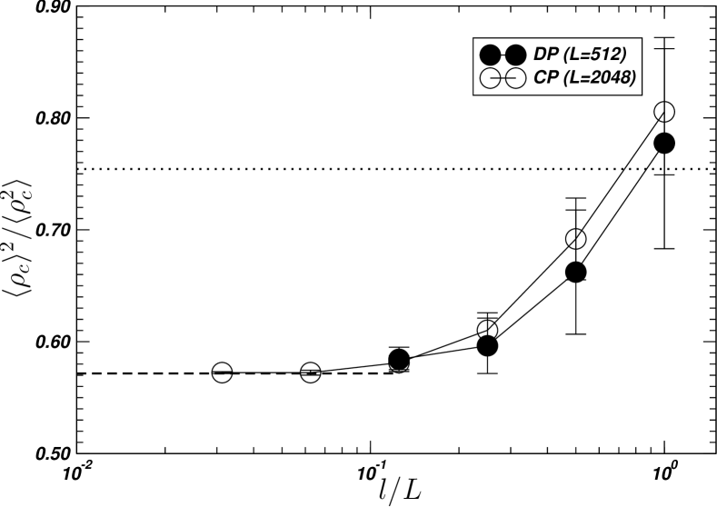
Figure 3: The moment ratio $R_{c}(l;L)=\left\langle\rho_{c}\right\rangle^{2}(l;L)/\left\langle\rho_{c}^{2}\right\rangle(l;L)$ for the two-dimensional CP and DP. For $l>l_{0}$ (here $l_{0}=64$ was needed for satisfactory results) the values coincide for both models, as expected by universality. The dashed line shows the expected assymptote for small $l/L$, whereas $l/L=1$ is consistent with the finite size scaling result $R_{c}(L;L)=0.7543(4)$ (dotted line) reported in [21].

3.5 Surrogate data

The proposed method can be put to test and compared to others using surrogate data, that is data generated in a computer implementation of, for example, the contact process, mimicking real-world data as they would be obtained in physical or biological systems. In contrast to the simulation data used above, such data consists of a single realisation, as if one was to analyse a satelitte image or field data.

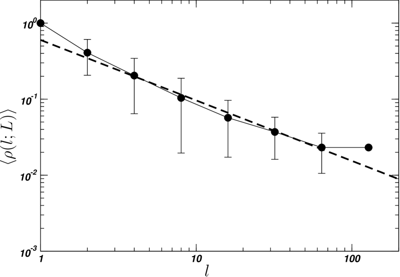
Figure 4: Conditional box scaling of the activity as measured in a single instance of the two-dimensional CP as surrogate data. The dashed line indicates the expected scaling, which fits the data very well.

Figure 4 shows the conditional box scaling of the activity $\left\langle\rho\right\rangle_{c}(l;L)$ for a single realisation of a two-dimensional system of linear size $L=128$ as a function of the box size $l$. The slope of $\left\langle\rho\right\rangle_{c}(l;L)$ is compared to $l^{-\beta/\nu_{\perp}}$ (thick dashed line) and fits very well. No errorbar can be given for $l=L$, as there is only one such sample, the remaining errorbars are estimated from the variance of the corresponding sample of size $(L/l)^{2}$, assuming independence.

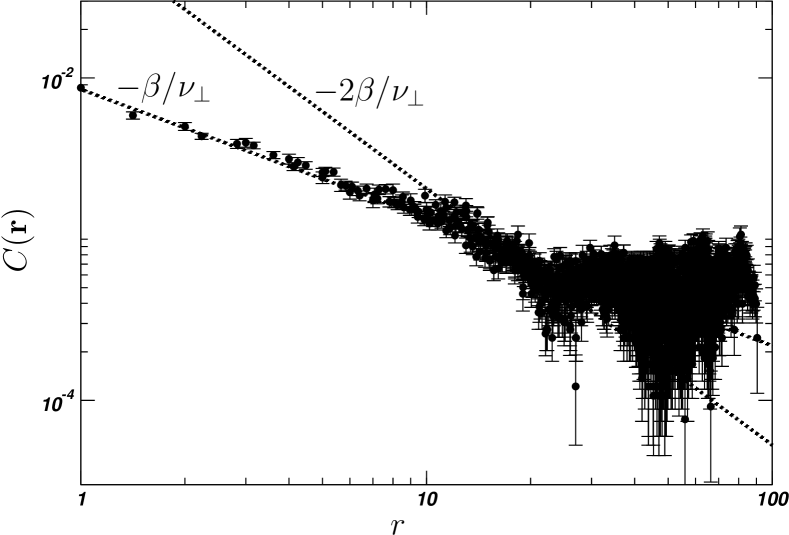
Figure 5: The two point correlation function (see Equation (7)) as measured in a single instance of the two-dimensional CP as surrogate data. The error is underestimated by assumed independence of the samples. The dotted lines indicate the expected scaling. The steeper one corresponds to what is found in equilibrium critical phenomena, which is superseeded by the shallower one. This line, with exponent $-\beta/\nu_{\perp}$ captures the behaviour for not too large distances quite well.

For comparison, Figure 5 is a double logarithmic plot of the two point correlation function

$$C(\mathbf{r})=L^{-2}\sum_{\mathbf{r}^{\prime}}I(\mathbf{r}^{\prime})I(\mathbf{r}^{\prime}+\mathbf{r})-\left(L^{-2}\sum_{\mathbf{r}^{\prime}}I(\mathbf{r}^{\prime})\right)^{2}$$ (7)

as a function of the absolute distance $|\mathbf{r}|$. Here $I(\mathbf{r})$ indicates occupation of site $\mathbf{r}$ and the sums run over all $L^{2}$ sites $\mathbf{r}^{\prime}$. It is taken from the same sample as Figure 4, using the translational invariance and the eight-fould symmetry of a square. Nevertheless, the data is comparatively noisy. Naïve scaling arguments along the lines of equilibrium phase transitions [22] suggest an asymptote $C(\mathbf{r})\propto|\mathbf{r}|^{-d+2-\eta}=|\mathbf{r}|^{-2\beta/\nu_{\perp}}$. In Figure 5 it is shown as a thick dotted line, but this asymptote is compatible with the data only in a narrow, noisy intermediate regime.

The correct scaling behaviour of the correlation function however is $C(\mathbf{r})\propto|\mathbf{r}|^{-\beta/\nu_{\perp}}$, which is found by imposing that $C(\mathbf{r})/\left\langle\rho\right\rangle_{u}$ does not scale in $L$ [23] (as it would, for example, in equlibrium phase transitions, consistent with [24]). Though still noisy, the data for small $r$ shown in Figure 5, indeed is much better compatible with a scaling exponent of $-\beta/\nu_{\perp}=-0.795(6)$.

Box scaling of the order parameter is due to the correlations captured in the two-point correlation function, as can be seen directly by deriving the variance $\sigma^{2}_{u}\left(\rho\right)(l;L)$ from $C(\mathbf{r})$,

$$\sigma^{2}_{u}\left(\rho\right)(l;L)=l^{-2d}\int_{l^{d}}\mathchoice{\!\!\mathrm{d}^{d}r\,}{\!\mathrm{d}^{d}r\,}{\!\mathrm{d}^{d}r\,}{\!\mathrm{d}^{d}r\,}\int_{l^{d}}\mathchoice{\!\!\mathrm{d}^{d}r^{\prime}\,}{\!\mathrm{d}^{d}r^{\prime}\,}{\!\mathrm{d}^{d}r^{\prime}\,}{\!\mathrm{d}^{d}r^{\prime}\,}C(\mathbf{r}-\mathbf{r}^{\prime})\propto l^{-\beta/\nu_{\perp}}$$ (8)

consistent with $\sigma^{2}_{u}\left(\rho\right)(l;L)\propto l^{-\beta/\nu_{\perp}}$ as observed earlier. Box scaling therefore can be regarded as an elegant form of extracting the correlations from the correlation function. From that point of view, the advantage of box scaling over a direct investigation of the two-point correlation function is merely down to its simplicity: Box scaling is well understood theoretically and easy to implement in an experiment, in field work or in a computer simulation.

As a final remark, the quality of the surrogate data shows a strong time dependence. Starting from a randomly occupied lattice, chosing too short an equilibration time leads to a lack of correlations, with the system still being dominated by the independent, random initialisation. Waiting too long, on the other hand, means that the system is likely to be low in activity and just about to die out completely, producing sparse and biased results.

4 Discussion

A block scaling analysis could provide a practical method to overcome the problem of limited availability of data in natural systems and allow the analysis of a natural system’s scaling behaviour without the need of an entire time series. Block scaling effectively is a form of sub-sampling and the analysis utilises the universal scaling with changing block size, which is characterised in the present work. As it turns out, in order to obtain block scaling as known from equilibrium critical phenomena, one has to use a conditional ensemble, where moments of the activity in a block enter the average only conditional to non-vanishing activity. The situation in absorbing state phase transitions therefore is very different from what is expected from equilibrium critical phenomena, where no additional condition is needed in order to obtain box scaling corresponding to finite size scaling.

Box scaling effectively measures the correlations between finite boxes throughout the system. In (near-)equilibrium systems, i.e. systems with a Hamiltonian, at the critical point, the probability density function of the order parameter is symmetric around $0$ due to the symmetry of the Hamiltonian. As contributions with opposite signs cancel, fluctuations decrease with increasing box size and consequently, the box averaged (absolute) order parameter and its variance decline.

In absorbing state systems, this mechanism does not exist: The local order parameter is non-negative and therefore cannot cancel out. In an unconditional ensemble the order parameter does not change with block size and fluctuations about the mean are not symmetric. For the order parameter to vanish, its fluctuations must vanish as well. Nevertheless, introducing the conditional ensemble restores the behaviour of (near-)equilibrium systems.

Within the conditional ensemble, the scaling functions of the observables considered converge to a finite value for small arguments, so that the cumulants scale in $l$ with the expected exponents, $\left\langle\rho\right\rangle_{c}\propto l^{-\beta/\nu_{\perp}}$ and $\sigma^{2}_{c}\left(\rho\right)\propto l^{-2\beta/\nu_{\perp}}$ for sufficiently small $l/L$. Moreover, the moment ratio $\left\langle\rho\right\rangle_{c}^{2}/\left\langle\rho^{2}\right\rangle_{c}$ is universal and converges to a non-zero, universal value for sufficiently small $l/L$.

This is not the case in the unconditional ensemble: The scaling functions are power-laws themselves and therefore the moments display an unconventional scaling. As a consequence, the average activity is constant in $l$, while its variance scales like $\sigma^{2}_{u}\left(\rho\right)\propto l^{-\beta/\nu_{\perp}}L^{-\beta/\nu_{\perp}}$ for small $l/L$. In addition, the moment ratio $\left\langle\rho\right\rangle_{u}^{2}/\left\langle\rho^{2}\right\rangle_{u}$ vanishes asymptotically in small $l/L$. The unconventional scaling of the unconditional ensemble is due to the existence of the translational symmetry which is not present in the conditional ensemble. This symmetry causes the lack of scaling of the first moment, which is connected to that of all other moments through (1):

The ratio of any unconditional moment and its conditional counterpart is the fraction of active blocks $a(l;L)$; this quantity itself displays universal behaviour in the ratio $l/L$. Any unconditional moment can be derived from the corresponding conditional one and vice versa, by multiplying and dividing by $a(l;L)$ respectively.

The key advantage of the conditional ensemble is the scaling of the first moment $\left\langle\rho\right\rangle_{c}$, which is usually the easiest to determine, carrying the smallest statistical error. In the unconditional ensemble, the first moment does not scale at all. Moreover, the moment ratio $\left\langle\rho\right\rangle_{c}^{2}/\left\langle\rho^{2}\right\rangle_{c}$ converges to a finite, universal value, which again is a quantity with a comparatively small statistical error. The hope is to use these observables in experimental situations where the system is guaranteed to be at the critical point.

References

- [1] Janssen H K 1981 Z. Phys. B 42 151–154
- [2] Grassberger P 1982 Z. Phys. B 47 365–374
- [3] Hinrichsen H 2000 Braz. J. Phys. 30 69–82 (Preprint cond-mat/9910284)
- [4] Takeuchi K A, Kuroda M, Chaté H and Sano M 2007 Phys. Rev. Lett. 99 234503–1–4
- [5] Binder K 1981 Z. Phys. B 43 119–140
- [6] Lübeck S and Heger P C 2003 Phys. Rev. E 68 056102–1–11
- [7] de Oliveira M M and Dickman R 2005 Phys. Rev. E 71 016129–1–5
- [8] Pruessner G 2008 Phys. Rev. E 76 061103–1–4 (Preprint arXiv:0712.0979v1)
- [9] Wegner F J 1972 Phys. Rev. B 5 4529–4536
- [10] Fisher M E and Barber M N 1972 Phys. Rev. Lett. 28 1516–1519
- [11] Barber M N 1983 Phase Transitions and Critical Phenomena vol 8 ed Domb C and Lebowitz J L (New York: Academic Press)
- [12] Privman V, Hohenberg P C and Aharony A 1991 Phase Transitions and Critical Phenomena vol 14 ed Domb C and Lebowitz J L (New York: Academic Press) chap 1, pp 1–134
- [13] Marro J and Dickman R 1999 Nonequilibrium Phase Transitions in Lattice Models (New York: Cambridge University Press)
- [14] Stauffer D and Aharony A 1994 Introduction to Percolation Theory (London: Taylor & Francis)
- [15] Harris T E 1974 Ann. Prob. 2 969–988
- [16] Grassberger P 1989 J. Phys. A: Math. Gen. 22 3673–3679
- [17] Dickman R 1999 Phys. Rev. E 60 R2441–R2444
- [18] Grassberger P and Zhang Y C 1996 Physica A 224 169–179
- [19] Lübeck S and Willmann R D 2005 Nucl. Phys. B 718 341–361
- [20] Huang K 1987 Statistical Mechanics (Chichester: John Wiley & Sons)
- [21] Dickman R and Kamphorst Leal da Silva J 1998 Phys. Rev. E 58 4266–4270
- [22] Lübeck S 2004 Int. J. Mod. Phys. B 18 3977–4118
- [23] Dickman R and Martins de Oliveira M 2005 Physica A 357 134–141
- [24] Grassberger P and de la Torre A 1979 Ann. Phys. 122 373–396