The effects of the little Higgs models on $t\bar{t}h^{0}$ production via $\gamma\gamma$ collision at linear colliders

Abstract

In the frameworks of the littlest Higgs($LH$) model and its extension with T-parity($LHT$), we studied the associated $t\bar{t}h^{0}$ production process $e^{+}e^{-}\to\gamma\gamma\to t\bar{t}h^{0}$ at the future $e^{+}e^{-}$ linear colliders up to QCD next-to-leading order. We present the regions of $\sqrt{s}-f$ parameter space in which the $LH$ and $LHT$ effects can and cannot be discovered with the criteria assumed in this paper. The production rates of process $\gamma\gamma\to t\bar{t}h^{0}$ in different photon polarization collision modes are also discussed. We conclude that one could observe the effects contributed by the $LH$ or $LHT$ model on the cross section for the process $e^{+}e^{-}\to\gamma\gamma\to t\bar{t}h^{0}$ in a reasonable parameter space, or might put more stringent constraints on the $LH$/$LHT$ parameters in the future experiments at linear colliders.

PACS: 12.60.Cn, 14.80.Cp, 14.65.Ha

I Introduction

The standard model($SM$)[1][2] of elementary particle physics provides a remarkably successful description of high energy physics phenomena at the energy scale up to $100~{}GeV$. Despite its tremendous success, the mechanism of electroweak symmetry breaking ($EWSB$) remains the most prominent mystery in current particle physics, and the Higgs boson mass suffers from an instability under radiative corrections leading to the ”hierarchy problem” between the electroweak scale and the $10~{}TeV$ cut-off scale $\Lambda$. The study of the $EWSB$ and the ”hierarchy problem” motivate many research works on the extensions of the $SM$. Recently, the little Higgs models have drawn a lot of interests as they offer an alternative approach to solve the ”hierarchy problem”[3], and were proposed as one kind of models of $EWSB$ without fine-tuning in which the Higgs boson is naturally light as a result of non-linearly realized symmetry[4]-[10]. The most economical model of them is the littlest Higgs($LH$) model, which is based on an $SU(5)/SO(5)$ nonlinear sigma model[7]. The key feature of this kind of models is that the Higgs boson is a pseudo-Goldstone boson of a global symmetry, which is spontaneously broken at some higher scale $f$, and thus is naturally light. The $EWSB$ is induced by a Coleman-Weinberg potential, which is generated by integrating out the heavy degrees of freedom.

In the $LH$ model without T-parity, a set of new heavy gauge bosons ($A_{H},Z_{H},W_{H}$) and a new heavy vector-like quark ($T$) are introduced which just cancel the quadratic divergences of Higgs self-energy induced by $SM$ gauge boson loops and the top quark loop, respectively. However, it has been shown that the $LH$ model without T-parity suffers from severe constraints from the precision electroweak data, which would require raising the masses of new particles to be much higher than $1~{}TeV$[11]. To avoid this problem, T-parity is introduced into the $LH$ model, which is called the littlest Higgs model with T-parity ($LHT$)[12]. In the $LHT$ model, the $SM$ particles are T-even and the most of the new heavy particles are T-odd. Thus, the $SM$ gauge bosons cannot mix with the new gauge bosons, and the electroweak precision observables are not modified at tree level. Beyond the tree level, small radiative corrections induced by the model to precision data still allow the symmetry breaking scale $f$ to be significantly lower than $1~{}TeV$[13]. In the top-quark sector, the $LHT$ model contains a T-odd and a T-even partner of the top quark. The T-even partner of the top quark mixes with top quark and cancels the quadratic divergence from top quark loop in the contributions to Higgs boson mass. Consequently, the $LHT$ model could induce abundant new phenomenology in present and future experiments.

In previous works, it is concluded that the LHC has great potential to discover directly the new particles predicted by the little Higgs models up to multi-TeV mass scale, such as the colored vector-like quark $T$, heavy gauge bosons and so on, in Refs.[14][15] and the references therein. After the new particles or interactions in the little Higgs models had been directly discovered at the LHC experiment, the International Linear Collider(ILC) would then play an important role in the detailed study of these new phenomena and accurate measurement of the interactions in the little Higgs models.

The precise measurement of the process of $t\bar{t}h^{0}$ production at the ILC is particularly important for probing the Yukawa coupling between top-quarks and the Higgs boson with intermediate mass. Actually, the $t\bar{t}h^{0}$ production can be first detected at the CERN LHC and further precisely measured at the ILC. It was pointed out that the $t-\bar{t}-h^{0}$ Yukawa coupling in $e^{+}e^{-}\to t\bar{t}h^{0}$ process can be measured to $6-8\%$ accuracy with integral luminosity $1000~{}fb^{-1}$ at an $e^{+}e^{-}$ linear collider (LC) with $\sqrt{s}=1~{}TeV$[16, 17]. The accurate predictions for the process $e^{+}e^{-}\to t\bar{t}h^{0}$ at linear colliders in $e^{+}e^{-}$ collision mode have been intensively discussed in many literatures[18]-[24]. Chong-Xing Yue, et al., studied the $e^{+}e^{-}\to t\bar{t}h^{0}$ process in the $LH$ and $LHT$ model at $ILC$[25, 26]. They found that in the parameter space preferred by the electroweak precision data in the $LH$ model($f=1\sim 2~{}TeV$, $c=0\sim 0.5$, $c^{\prime}=0.62\sim 0.73$)[27], the absolute value of the relative correction $\delta\sigma/\sigma^{SM}$ can be larger than $5\%$, while in the $LHT$ model as long as $f\leq 1~{}TeV$ and $c_{\lambda}=0.1\sim 0.9$, the value of $|\delta\sigma/\sigma^{SM}|$ can be larger than $7\%$. That means in these parameter space the $LH/LHT$ model effects might be observed in the future $ILC$ experiment. Except the $e^{+}e^{-}$ collision mode, an $e^{+}e^{-}$ LC can also be operated as a $\gamma\gamma$ collider. This is achieved by using Compton backscattered photons in the scattering of intense laser photons on the initial $e^{+}e^{-}$ beams. Generally $e^{+}e^{-}$ collider has the advantage that the luminosity is higher than $\gamma\gamma$ collider, for example, ${\cal L}_{\gamma\gamma}\sim 0.15-0.2~{}{\cal L}_{e^{+}e^{-}}$ or even $0.3-0.5~{}{\cal L}_{e^{+}e^{-}}$(through reducing emittance in the damping rings)[28], but the polarization technique for photon is much simpler than electron and the LC with continuous colliding energy spectrum of $\gamma\gamma$ will be helpful to pursue new particles. Therefore, LC can provide anther possibility to measure precisely the $t-\bar{t}-h^{0}$ coupling in $\gamma\gamma$ collision mode. Similar with the study on the process $e^{+}e^{-}\to t\bar{t}h^{0}$ at LC, the evaluation of radiative corrections to the process $\gamma\gamma\to t\bar{t}h^{0}$ is also significant for the accurate experimental measurements of $t-\bar{t}-h^{0}$ Yukawa coupling at LC. In the Ref.[29], the calculations of the cross sections for $\gamma\gamma\to t\bar{t}h^{0}$ and $e^{+}e^{-}\to\gamma\gamma\to t\bar{t}h^{0}$ process including NLO QCD and one-loop electroweak corrections in the $SM$ were presented.

Due to the fact that it is speculated that the Yukawa coupling between top-quarks and Higgs boson is theoretically sensitive to the $LH$ and $LHT$ contributions, and the $t\bar{t}h^{0}$ associated productions may be favorable for probing these little Higgs models. In this paper we study the reach of the ILC operating in $\gamma\gamma$ collision mode to probe the $LH$ and $LHT$ model in the process $e^{+}e^{-}\to\gamma\gamma\to t\bar{t}h^{0}$ at the QCD next-to-leading order. The paper is organized as follows. In Sec. 2 we give a brief review of the $LH$ and $LHT$ model. In Section 3, we present the notations and analytical calculation of the process $e^{+}e^{-}\to\gamma\gamma\to t\bar{t}h^{0}$ including the QCD NLO radiative corrections. The numerical result and discussions are presented in Section 4. Finally the conclusions are given.

II Related theory of the $LH$ and $LHT$ models

Before our calculations, we will briefly recapitulate the $LH$ and $LHT$ model which are relevant to the analysis in this work. For the detailed description of these two models, one can refer to Refs.[7, 12]. The littlest Higgs($LH$) model is based on the $SU(5)/SO(5)$ non-linear sigma model[30]. In this model, the SM fermions acquire their masses via the usual Yukawa interactions. However, to cancel the large quadratic divergence in the Higgs boson mass due to the heavy top quark Yukawa interaction in the $SM$, a pair of new colored weak singlet Weyl fermions $\tilde{t}$ and $\tilde{t}^{\prime c}$ is required in addition to the usual third family weak doublet $q_{3}=(t_{3},b_{3})$ and weak singlet $u^{\prime c}_{3}$, where $u^{\prime c}_{3}$ and $\tilde{t}^{\prime c}$ are the corresponding right-handed singlets. And the third family $SM$ quark doublet is replaced by a chiral triplet field $\chi=(b_{3},t_{3},\tilde{t})$. The Lagrangian generating the Yukawa couplings between pseudo-Goldstone bosons and the heavy vector-like fermion pair in the $LH$ model is taken the form as[30]:

$${\cal L}_{Y} = \frac{1}{2}\lambda_{1}f\epsilon_{ijk}\epsilon_{xy}\chi_{i}\Sigma_{jx}\Sigma_{ky}u^{\prime c}_{3}+\lambda_{2}f\tilde{t}\tilde{t}^{\prime c}+h.c.$$ (2.1)

where $\epsilon_{ijk}$ and $\epsilon_{xy}$ are antisymmetric tensors. $i$, $j$, $k$ run through 1, 2, 3 and $x$, $y$ run through 4, 5. $\lambda_{1}$ and $\lambda_{2}$ are the coupling constants. By expanding above Lagrangian, we get the physical states of the top quark $t$ and a new heavy-vector-like quark $T$, and obtain the usual mass result for the eigenvalues corresponding to the top quark $t$ and the heavy top $T$ which are up to order ${\cal O}(v/f)$:

$$m_{t}=\frac{\lambda_{1}\lambda_{2}}{\sqrt{\lambda_{1}^{2}+\lambda_{2}^{2}}}\;v\;,\;\;\;m_{T}=\sqrt{\lambda_{1}^{2}+\lambda_{2}^{2}}\;f.$$ (2.2)

From the Lagrangian shown in Eq.(2.1), the couplings in the $LH$ model concerned in the calculation of $\gamma\gamma\to t\bar{t}h^{0}$ process can be expressed as:

$$g_{t\bar{t}h}^{LH} = -i\frac{m_{t}}{v}\left[1-\frac{1}{2}s_{0}^{2}+\frac{v}{f}\frac{s_{0}}{\sqrt{2}}-\frac{2v^{2}}{3f^{2}}+\frac{v^{2}}{f^{2}}c_{\lambda}^{2}(1+c_{\lambda}^{2})\right]$$ (2.3)

$$g_{T\bar{T}h}^{LH} = -i\frac{\lambda_{1}^{2}}{\sqrt{\lambda_{1}^{2}+\lambda_{2}^{2}}}\left(1+c_{\lambda}^{2}\right)\frac{v}{f},$$ (2.4)

where $v$ is one of the vacuum expectation values($v=(\sqrt{2}G_{F})^{-1/2}=246.22~{}GeV$), $c_{\lambda}$ is define as $c_{\lambda}=\frac{\lambda_{1}}{\sqrt{\lambda_{1}^{2}+\lambda_{2}^{2}}}$[31, 32]($\lambda_{1}$ and $\lambda_{2}$ are the Yukawa coupling parameters), $s_{0}$ is the scalar mixing angle of Higgs fields, $s_{0}\simeq 2\sqrt{2}\frac{v^{\prime}}{v}=\frac{xv}{\sqrt{2}f}\sim\mathcal{O}(v/f)$, where we define $x\equiv 4f\frac{v^{\prime}}{v^{2}}$[33].

Recently, the symmetry structure of the the $LH$ model was enlarged by introducing an additional discrete symmetry, T-parity, in analogy to the R-parity in the minimal supersymmetric standard model($MSSM$)[12]. The T-parity interchanges the two subgroups $[SU(2)\times U(1)]_{1}$ and $[SU(2)\times U(1)]_{2}$ of $SU(5)$. Due to T-parity, the new gauge bosons do not mix with the $SM$ gauge bosons and thus the new particles don’t generate corrections to precision electroweak observables at tree level. The top quark sector contains a T-even and T-odd partner, with the T-even one mixing with top quark and cancelling the quadratic divergence contribution of top quark to Higgs boson mass. The mass of the T-even partner (denoted as $T$) is the same as shown in Eq.(2.2), while the mass of the T-odd partner (denoted as $T_{-}$) is given by

$$m_{T_{-}}=\lambda_{2}f,$$ (2.5)

The mixing of $T$-quark with the top quark will alter the $SM$ top quark couplings, and the relevant couplings in the $LHT$ model using in our calculation are given as

$$g_{t\bar{t}h}^{LHT} = -i\frac{m_{t}}{v}\left[1-\left(\frac{3}{4}-c_{\lambda}^{2}+c_{\lambda}^{4}\right)\frac{v^{2}}{f^{2}}\right],$$ (2.6)

$$g_{T\bar{T}h}^{LHT} = {i\frac{m_{t}c_{\lambda}s_{\lambda}}{f}},$$ (2.7)

where $s_{\lambda}=\sqrt{1-c_{\lambda}^{2}}$, and the Feynman rules for the third generation quarks-gluon($\gamma$) couplings in both $LH$ and $LHT$ models, have the same forms as the $gf\bar{f}(\gamma f\bar{f})$ couplings in the $SM$.

Moreover, the top quark mass is already obtained by experiment, then we can get the parameter relation from Eq. (2.2) as deduced in Ref.[30]

$$\frac{1}{\lambda_{1}^{2}}+\frac{1}{\lambda_{2}^{2}}\approx\frac{v^{2}}{{m_{t}}^{2}}\approx 2.$$ (2.8)

III Analytical calculations

III.1 LO calculations of the $\gamma\gamma\to t\bar{t}h^{0}$ subprocess

We denote the subprocess $\gamma\gamma\to t\bar{t}h^{0}$ as

$$\gamma(p_{1},\lambda_{1})+\gamma(p_{2},\lambda_{2})\to t(k_{1})+\bar{t}(k_{2})+h^{0}(k_{3}).$$ (3.1)

where the four-momenta of incoming electron and positron are denoted as $p_{1}$ and $p_{2}$, and the four-momenta of outgoing top-quark, anti-top-quark and Higgs boson are represented as $k_{1}$, $k_{2}$ and $k_{3}$ respectively, $\lambda_{1,2}$ are the polarizations of incoming photons. The tree-level t-channel Feynman diagrams are shown in Fig.1, the u-channel with the exchange of the two incoming photons are not shown. There Higgs boson radiates from the internal or external top-quark lines, so the cross section should be proportional to factor $g_{t\bar{t}h}^{2}$. Consequently, this process can be used to probe the $t-\bar{t}-h^{0}$ Yukawa coupling directly.

Figure 1: The lowest order diagrams for the $\gamma\gamma\to t\bar{t}h^{0}$ subprocess.

The amplitudes of the corresponding t-channel Feynman diagrams (shown in Fig.1(a-c)) for the subprocess $\gamma\gamma\to t\bar{t}h^{0}$ are expressed as

$${\cal M}^{(a)}_{t}=-\frac{e^{3}Q_{t}^{2}m_{t}}{2m_{W}\sin\theta_{W}}\frac{1}{(k_{1}-p_{1})^{2}-m_{t}^{2}}\frac{1}{(p_{2}-k_{2})^{2}-m_{t}^{2}}\cdot~{}~{}~{}~{}$$

$$\times\bar{u}(k_{1})\hbox to0.0pt{/\hss}{\epsilon}(p_{1},\lambda_{1})(\hbox to0.0pt{/\hss}{k}_{1}-\hbox to0.0pt{/\hss}{p}_{1}+m_{t})(\hbox to0.0pt{/\hss}{p}_{2}-\hbox to0.0pt{/\hss}{k}_{2}+m_{t})\hbox to0.0pt{/\hss}{\epsilon}(p_{2},\lambda_{2})v(k_{2}),$$ (3.2)

$${\cal M}^{(b)}_{t}=-\frac{e^{3}Q_{t}^{2}m_{t}}{2m_{W}\sin\theta_{W}}\frac{1}{(k_{1}-p_{1})^{2}-m_{t}^{2}}\frac{1}{(k_{2}+k_{3})^{2}-m_{t}^{2}}\cdot~{}~{}~{}~{}$$

$$\times\bar{u}(k_{1})\hbox to0.0pt{/\hss}{\epsilon}(p_{1},\lambda_{1})(\hbox to0.0pt{/\hss}{k}_{1}-\hbox to0.0pt{/\hss}{p}_{1}+m_{t})\hbox to0.0pt{/\hss}{\epsilon}(p_{2},\lambda_{2})(-\hbox to0.0pt{/\hss}{k}_{2}-\hbox to0.0pt{/\hss}{k}_{3}+m_{t})v(k_{2}),$$ (3.3)

$${\cal M}^{(c)}_{t}=-\frac{e^{3}Q_{t}^{2}m_{t}}{2m_{W}\sin\theta_{W}}\frac{1}{(k_{1}+k_{3})^{2}-m_{t}^{2}}\frac{1}{(p_{2}-q_{2})^{2}-m_{t}^{2}}\cdot~{}~{}~{}~{}$$

$$\times\bar{u}(k_{1})(\hbox to0.0pt{/\hss}{k}_{1}+\hbox to0.0pt{/\hss}{k}_{3}+m_{t})\hbox to0.0pt{/\hss}{\epsilon}(p_{1},\lambda_{1})(\hbox to0.0pt{/\hss}{p}_{2}-\hbox to0.0pt{/\hss}{k}_{2}+m_{t})\hbox to0.0pt{/\hss}{\epsilon}(p_{2},\lambda_{2})v(k_{2}),$$ (3.4)

where $Q_{t}=2/3$ and the corresponding amplitudes of the u-channel Feynman diagrams of the subprocess $\gamma\gamma\to t\bar{t}h^{0}$ can be obtained by exchanging $\gamma(p_{1},\lambda_{1})\leftrightarrow\gamma(p_{2},\lambda_{2})$.

$${\cal M}^{(a)}_{u}={\cal M}^{(a)}_{t}(p_{1},\lambda_{1}\leftrightarrow p_{2},\lambda_{2}), {\cal M}^{(b)}_{u}={\cal M}^{(b)}_{t}(p_{1},\lambda_{1}\leftrightarrow p_{2},\lambda_{2}),$$ (3.5)

$${\cal M}^{(c)}_{u}={\cal M}^{(c)}_{t}(p_{1},\lambda_{1}\leftrightarrow p_{2},\lambda_{2}).$$

The total amplitude at the lowest order is the summation of the above amplitudes.

$${\cal M}_{0}=\sum_{i=a,b}^{c}\sum_{j=u}^{t}{\cal M}^{(i)}_{j}.$$ (3.6)

The cross section of the subprocess $\gamma\gamma\to t\bar{t}h^{0}$ in unpolarized photon collision mode at the tree-level can be obtained by integrating over the phase space,

$$\hat{\sigma}_{0}(\hat{s})=\frac{(2\pi)^{4}N_{c}}{4|\vec{p}_{1}|\sqrt{s}}\int{\rm d}\Phi_{3}\overline{\sum_{{\rm spin}}}|{\cal M}_{0}|^{2},$$ (3.7)

where $N_{c}=3$ and $\vec{p}_{1}$ is the c.m.s. momentum of one initial photon, $d\Phi_{3}$ is the three-body phase space element, and the bar over summation recalls averaging over initial spins[34].

III.2 Calculations of the QCD NLO corrections of the $\gamma\gamma\to t\bar{t}h^{0}$ subprocess

The ${\cal O}(\alpha_{s})$ QCD NLO Feynman diagrams of the subprocess $\gamma\gamma\to t\bar{t}h^{0}$ are generated by ${\it FeynArts}~{}3$ [35]. The QCD NLO Feynman diagrams can be divided into self-energy, vertex, box, pentagon and counter term diagrams. We find there exist the QCD one-loop diagrams which include $T$-quark/$T_{\pm}$-quark in loops for the $LH$/$LHT$ model, but the total contributions from these diagrams are vanished in both models separately. The representative pentagon Feynman diagrams which generate amplitudes including five-point integrals of rank 4 are shown in Fig.2. The amplitude of the subprocess $\gamma\gamma\to t\bar{t}h^{0}$ including virtual QCD corrections to ${\cal O}(\alpha_{s})$ order can be expressed as

$${\cal M}_{QCD}={\cal M}_{0}+{\cal M}_{QCD}^{vir},$$ (3.8)

where ${\cal M}_{QCD}^{vir}$ is the renormalized amplitude contributed by the QCD one-loop Feynman diagrams, the QCD renormalizations of top-quark wave function, mass and $t-\bar{t}-h^{0}$ Yukawa coupling. There we define the relevant QCD renormalization constants as

$$m_{t,0}=m_{t}+\delta m_{t(g)},~{}~{}t_{0}^{L}=\left(1+\frac{1}{2}\delta Z_{t(g)}^{L}\right)t^{L},$$

$$t_{0}^{R}=\left(1+\frac{1}{2}\delta Z_{t(g)}^{R}\right)t^{R},~{}~{}g_{t\bar{t}h}^{0}=g_{t\bar{t}h}\left(1+\frac{\delta m_{t(g)}}{m_{t}}\right).$$ (3.9)

In analogy to the calculation of the QCD renormalization constants in Ref.[29], we adopt the on-mass-shell renormalization condition to get the QCD contributed parts of the renormalization constants, $\delta m_{t(g)}$ and $\delta Z_{t(g)}^{L,R}$.

Figure 2: The representative QCD one-loop diagrams which produce amplitudes include five-point tensor integrals of rank 4.

The virtual QCD corrections contain both ultraviolet (UV) and soft infrared (IR) divergences. We adopt the dimensional regularization($DR$) to regularize the UV divergences in loop integrals, and to isolate IR singularities. After renormalization procedure, the virtual correction part of the cross section is UV-finite. The IR divergences from the one-loop diagrams involving virtual gluon can be cancelled by adding the soft real gluon emission corrections by using the phase space slicing method (PSS)[36]. The real gluon emission process is denoted as

$$\gamma(p_{1},\lambda_{1})+\gamma(p_{2},\lambda_{2})\rightarrow t(k_{1})+\bar{t}(k_{2})+h^{0}(k_{3})+g(k),$$ (3.10)

where a real gluon radiates from the internal or external top(anti-top) quark line. The phase space for $\gamma\gamma\to t\bar{t}h^{0}+g$ process is divided into two parts which behave soft and hard gluon emission natures, respectively.

$$\Delta\hat{\sigma}_{real}^{QCD}=\Delta\hat{\sigma}_{soft}^{QCD}+\Delta\hat{\sigma}_{hard}^{QCD}.$$ (3.11)

Finally the UV and IR finite total cross section of the subprocess $\gamma\gamma\to t\bar{t}h^{0}$ including the ${\cal O}(\alpha_{s})$ QCD corrections is obtained as

$$\hat{\sigma}^{QCD}=\hat{\sigma}_{0}+\Delta\hat{\sigma}^{QCD}=\hat{\sigma}_{0}+\Delta\hat{\sigma}_{{\rm vir}}^{QCD}+\Delta\hat{\sigma}_{{\rm real}}^{QCD}=\hat{\sigma}_{0}(1+\hat{\delta}^{QCD}),$$ (3.12)

where $\hat{\delta}^{QCD}$ is the QCD relative correction of order ${\cal O}(\alpha_{s})$.

III.3 Calculations of process $e^{+}e^{-}\to\gamma\gamma\to t\bar{t}h^{0}$

The hard photon beam of the $\gamma\gamma$ collider can be obtained by using the laser back-scattering technique at $e^{+}e^{-}$ linear collider [37, 38, 39]. For simplicity, in our calculations we ignore the possible polarization for the incoming electron and photon beams. We denote $\hat{s}$ and $s$ as the center-of-mass energies of the $\gamma\gamma$ and $e^{+}e^{-}$ systems, respectively. After calculating the cross section $\hat{\sigma}^{QCD}(\hat{s})$ for the subprocess $\gamma\gamma\to t\bar{t}h^{0}$ in unpolarized photon collision mode, the total cross section at an $e^{+}e^{-}$ linear collider can be obtained by folding $\hat{\sigma}^{QCD}(\hat{s})$ with the photon distribution function that is given in Ref.[40],

$$\sigma_{tot}(e^{+}e^{-}\to\gamma\gamma\to t\bar{t}h^{0},~{}s)=\int^{x_{max}}_{(2m_{t}+m_{h})/\sqrt{s}}dz\frac{d{\cal L}_{\gamma\gamma}}{dz}\hat{\sigma}^{QCD}(\hat{s}=z^{2}s).$$ (3.13)

The distribution function of photon luminosity $\frac{d{\cal L}_{\gamma\gamma}}{dz}$ is expressed as

$$\frac{d{\cal L}_{\gamma\gamma}}{dz}=2z\int_{z^{2}/x_{max}}^{x_{max}}\frac{dx}{x}f_{\gamma/e}(x)f_{\gamma/e}(z^{2}/x)$$ (3.14)

The energy spectrum of the back scattered photon in unpolarized incoming $e^{-}\gamma$ scattering is given by

$$f_{\gamma/e}(x)=\frac{1}{D(\xi)}\left[1-x+\frac{1}{1-x}-\frac{4x}{\xi(1-x)}+\frac{4x^{2}}{\xi^{2}(1-x)^{2}}\right],~{}~{}~{}(x<x_{max})$$ (3.15)

where the fraction of the energy of the incident electron carried by the back-scattered photon $x$, is expressed as $x=2\omega/\sqrt{s}$, and $x_{max}=2\omega_{max}/\sqrt{s}=\xi/(1+\xi)$. For $x>x_{max}$, $f_{\gamma/e}=0$. The function $D(\xi)$ is defined as

$$D(\xi)=(1-\frac{4}{\xi}-\frac{8}{\xi^{2}})\ln(1+\xi)+\frac{1}{2}+\frac{8}{\xi}-\frac{1}{2(1+\xi)^{2}}.$$ (3.16)

We denote $m_{e}$ and $\omega_{0}$ as electron mass and laser-photon energy respectively. The incoming electron energy is $\sqrt{s}/2$ and $\xi=\frac{2\omega_{0}\sqrt{s}}{{m_{e}}^{2}}$. In our evaluation, we choose $\omega_{0}$ such that it maximizes the backscattered photon energy without spoiling the luminosity through $e^{+}e^{-}$ pair creation. Then we have ${\xi}=2(1+\sqrt{2})$, $x_{max}\simeq 0.83$, and $D(\xi)\approx 1.84$[41].

IV Numerical results and discussions

In this section, we present some numerical results for both the $\gamma\gamma\to t\bar{t}h^{0}$ subprocess and $e^{+}e^{-}\to\gamma\gamma\to t\bar{t}h^{0}$ parent process in the littlest Higgs model and its extension model with T-parity(the $LH$ and $LHT$ model). In the numerical calculation, we take the input parameters as follows[34]

$$\alpha_{{\rm ew}}(0)^{-1}=137.03599911,~{}~{}~{}m_{W}=80.403~{}GeV,~{}~{}~{}m_{Z}=91.1876~{}GeV,$$

$$m_{t}=174.2~{}GeV,~{}~{}~{}\alpha_{s}(m_{Z})=0.117620.$$ (4.1)

The mixing parameter $s_{0}$, which appears in the $LH$ coupling(see Eq.(2.3)), is of the order ${\cal O}(v/f)$. We fix $s_{0}=\frac{v}{2f}$(It is equivalent to $x=\frac{1}{\sqrt{2}}$) in numerical evaluation, if there is no other statement. Then we still have additional four free $LH$/$LHT$ parameters ($f$, $c_{\lambda}$, $\sqrt{s}$, $m_{h}$) involved in our numerical calculations. C. Csaki, etal., performed a global fit to the precision data, and they found for generic regions of the parameter space of little Higgs models the bound on scale $f$ is several TeV, but there exist regions of parameter space in which $f$ can be relaxed to $1-2~{}TeV$ depending on the model variation and degree of tuning of model parameters[27]. Considering the fact as shown in our numerical results for the process $e^{+}e^{-}\to\gamma\gamma\to t\bar{t}h^{0}$ , the corrections from the $LH$ model are always less than $5\%$ when $f>2~{}TeV$. That means only the symmetry breaking scales $f$ up to $2~{}TeV$ are accessible in measuring the $LH$ model effects in $t\bar{t}h^{0}$ associated production. Then in the following numerical calculation in the $LH$ model we constraint the value of the scale $f$ being in the range of $1-2~{}TeV$. When it comes to the $LHT$ model, as the $SM$ gauge bosons can not mix with the new gauge bosons, and the electroweak precision observables are not modified at tree level, the symmetry breaking scale $f$ can be decreased to $500~{}GeV$, which will lead to rich phenomenology of the $LHT$ model in present and future high energy experiments. In this work we take the QCD renormalization scale $\mu$ being $(2m_{t}+m_{h})/2$, $c_{\lambda}\in[0.1,0.9]$ and the running strong coupling $\alpha_{s}(\mu^{2})$ being at the two-loop level($\overline{MS}$ scheme) with five active flavors.

The numerical results for the cross sections of $\gamma\gamma\to t\bar{t}h^{0}$ including QCD NLO radiative corrections versus $\gamma\gamma$ colliding energy $\sqrt{\hat{s}}$, are plotted in Figs.3(a-c) with $m_{h}=115$, $150$ and $200~{}GeV$ separately, where we take $f=1~{}TeV$ and $c_{\lambda}^{2}=0.8$. The curves correspond to the tree-level and QCD NLO corrected cross sections in the frameworks of the $SM$, $LH$ and $LHT$ model respectively, with $\sqrt{\hat{s}}$ running from the value little larger than the threshold $2m_{t}+m_{h}$ to $1.8~{}TeV$. Figs.3(a-c) show that the QCD corrections can increase (when $\sqrt{\hat{s}}<650~{}GeV$) or decrease(when $\sqrt{\hat{s}}>900~{}GeV$) the tree-level cross sections of subprocess $\gamma\gamma\to t\bar{t}h^{0}$ . As indicated in Fig.3(a), the curves for $m_{h}=115~{}GeV$ increase rapidly to their maximal cross section values, when the $\gamma\gamma$ colliding energy $\sqrt{\hat{s}}$ varies from threshold to the corresponding position of peak. As depicted in Fig.3(b) with $m_{h}=150~{}GeV$, all curves have platforms when $\sqrt{\hat{s}}$ is larger than $1~{}TeV$. In Fig.3(c) both Born and one-loop QCD corrected cross sections increase slowly in our plotted range of $\sqrt{\hat{s}}$. From Figs.3(a-c), we can also find that the tree-level and the NLO QCD corrected cross sections in the $LH$ model, is always larger than those in the other two models, while the cross section of the $LHT$ model is the smallest one among all of the three models.

Figure 3: The Born and the QCD NLO corrected cross sections of the process $\gamma\gamma\to t\bar{t}h^{0}$ as the functions of the c.m.s. energy $\sqrt{\hat{s}}$ of $\gamma\gamma$ collision with $m_{h}=115$, $150$ and $200~{}GeV$ respectively, in the conditions of $f=1~{}TeV$ and $c_{\lambda}^{2}=0.8$. (a) for $m_{h}=115~{}GeV$, (b) for $m_{h}=150~{}GeV$, (c) for $m_{h}=200~{}GeV$.

The tree-level and the QCD NLO corrected cross sections for the parent process $e^{+}e^{-}\to\gamma\gamma\to t\bar{t}h^{0}$ in the $SM$, $LH$ and $LHT$ model as the functions of the $e^{+}e^{-}$ colliding energy $\sqrt{s}$ in the conditions of $f=1~{}TeV$ and $c_{\lambda}^{2}=0.8$, are plotted in Figs.4(a-c) for $m_{h}=115~{}GeV$, $150~{}GeV$ and $200~{}GeV$ separately. As shown in the figures, both Born and QCD NLO corrected cross sections for each model go up with the increment of $\sqrt{s}$, and the QCD NLO radiative corrections for different value choices of $m_{h}$ can reduce or increase the Born cross sections in the plotted $\sqrt{s}$ range. The tendencies of all the curves in Figs.4(a), (b) and (c) are similar. The cross section including QCD NLO corrections in the $LH$($LHT$) model with $m_{h}=115~{}GeV$, can reach $1.5~{}fb(1.2~{}fb)$, and if we assume the integral luminosity of an $e^{+}e^{-}$ linear collider ${\cal L}_{e^{+}e^{-}}=1000~{}fb^{-1}$, we can accumulate about $1.5(1.2)\times 10^{3}$ $t\bar{t}h^{0}$ production events, thus it will be helpful in hunting for the $LH$/$LHT$ signals and the study of the Yukawa coupling.

Figure 4: The Born and QCD NLO corrected cross sections for the parent process $e^{+}e^{-}\to\gamma\gamma\to t\bar{t}h^{0}$ as the functions of c.m.s. energy $\sqrt{s}$ with $m_{h}=115$, $150$, $200~{}GeV$ respectively, where $f=1~{}TeV$ and $c_{\lambda}^{2}=0.8$. (a) is for $m_{h}=115~{}GeV$, (b) for $m_{h}=150~{}GeV$, (c) for $m_{h}=200~{}GeV$.

To illustrate the deviations of the cross sections in the $LH$/$LHT$ model for the process $e^{+}e^{-}\to\gamma\gamma\to t\bar{t}h^{0}$ from the $SM$ predictions, we plot $\Delta\sigma_{LH,LHT}(\equiv\sigma_{NLO}^{LH,LHT}-\sigma_{NLO}^{SM})$ as the functions of $e^{+}e^{-}$ colliding energy $\sqrt{s}$ with the conditions of $c_{\lambda}^{2}=0.8$ and $f=1(0.5)~{}TeV$(in the $LH$($LHT$) model) in Fig.5(a). The solid, dashed and dotted lines are for $m_{h}=115~{}GeV$, $150~{}GeV$ and $200~{}GeV$, respectively. For each line type, the upper line is for the case in the $LH$ model, while the lower one is in the $LHT$ model. From the figure, we can see that the absolute value of the cross section deviation $\Delta\sigma_{LH,LHT}$ raises with either the decrement of Higgs mass or the increment of $e^{+}e^{-}$ c.m.s energy $\sqrt{s}$. The deviations of the cross sections in the $LH$/$LHT$ model for the process $e^{+}e^{-}\to\gamma\gamma\to t\bar{t}h^{0}$ as the functions of the Higgs boson mass $m_{h}$ in the same conditions as in Fig.5(a) are shown in Fig.5(b). We can see from Fig.5(b) that for the curves of $\sqrt{s}=1000~{}GeV$, $1500~{}GeV$, the absolute deviations of the cross sections $|\Delta\sigma|$ can be larger than $0.05~{}fb$ when $m_{h}\in[100~{}GeV,~{}150~{}GeV]$(in the $LH$ model) and $m_{h}\in[100~{}GeV,~{}175~{}GeV]$(in the $LH$ model), and the effects could be observable in experiment. But when $m_{h}$ is larger than $300~{}GeV$, the effects from the $LH/LHT$ model become to be very small and are not sensitive to the Higgs boson mass.

Figure 5: (a) The $\Delta\sigma_{LH,LHT}$ dependence on $\sqrt{s}$ with $c_{\lambda}^{2}=0.8$ and $f=1(0.5)~{}TeV$(in the $LH(LHT)$ model) for the process $e^{+}e^{-}\to\gamma\gamma\to t\bar{t}h^{0}$ via $\gamma\gamma$ collision mode. (b) The $\Delta\sigma_{LH,LHT}$ dependence on $m_{h}$ with $c_{\lambda}^{2}=0.8$ and $f=1(0.5)~{}TeV$(for the $LH(LHT)$ model) for the process $e^{+}e^{-}\to\gamma\gamma\to t\bar{t}h^{0}$ via $\gamma\gamma$ collision mode.

In general, the extra contribution of the $LH$ or $LHT$ model to the cross section of the process $\gamma\gamma\to t\bar{t}h^{0}$ is proportional to a factor of $1/f^{2}$. In order to describe the $LH$/$LHT$ effects on the production cross section, we define the relative deviation parameters $R_{1}=\frac{\sigma_{NLO}^{LH}-\sigma_{NLO}^{SM}}{\sigma_{NLO}^{SM}}$ for the $LH$ model and $R_{2}=\frac{\sigma_{NLO}^{LHT}-\sigma_{NLO}^{SM}}{\sigma_{NLO}^{SM}}$ for the $LHT$ model, and depict $R_{1}$ and $R_{2}$ as the functions of symmetry breaking scale $f$ in Figs.6(a) and (b) separately. In Figs.6(a,b) we take $m_{h}=115~{}GeV$, $\sqrt{s}=800~{}GeV$, the mixing parameter $c_{\lambda}^{2}=0.5$, $0.8$, $0.9$, and $f$ being in the range of $[1~{}TeV,~{}3~{}TeV]$ for the $LH$ model, and $f\in[500~{}GeV,~{}2~{}TeV]$ for the $LHT$ model respectively. From Fig.6(a), we can see that the relative deviation parameter $R_{1}$ falls as $f$ increases, and when $c_{\lambda}^{2}\geq 0.8$, the values of $R_{1}$ are larger than $5\%$ in the range of symmetry breaking scale $f<1.5~{}TeV$, which might be detected in the future $LC$ experiments. Since the experimental constraint on symmetry breaking scale $f$ of the $LHT$ model can be lower than $1~{}TeV$, the absolute value of relative deviation parameter $R_{2}$ is generally larger than that in the $LH$ model with the $f$ in the range of $[500~{}GeV,~{}1~{}TeV]$. Similar to the result shown in Fig.6(a), Fig.6(b) shows that the absolute value of $R_{2}$ decreases quickly with the increment of symmetry breaking scale $f$, and the absolute values of $R_{2}$ in the $LHT$ model can be larger than $5\%$ in the range of $f<1.1~{}TeV$ for the three value choices of $c_{\lambda}$ ($c_{\lambda}^{2}=0.5$, $0.8$, $0.9$). We can see from the figures that the most distinctive difference between the relative deviation parameters $R_{1}$ and $R_{2}$, is that the $LH$ result $R_{1}$ is always positive, while the $LHT$ result $R_{2}$ is negative in our potted range of the symmetry breaking scale $f$. That is due to the $t-\bar{t}-h^{0}$ coupling difference between the $LHT$ and the $LH$ model.

Figure 6: The relative parameters $R_{1}$ and $R_{2}$ for the process $e^{+}e^{-}\to\gamma\gamma\to t\bar{t}h^{0}$ as the functions of the symmetry breaking scale $f$ for three different value choices of the mixing parameter $c_{\lambda}$, with $m_{h}=115~{}GeV$ and $\sqrt{s}=800~{}GeV$. (a) for $LH$ model and (b) for $LHT$ model

In order to show the dependence of the relative deviation $R_{1}$ on the parameter $x(\equiv 4f\frac{v^{\prime}}{v^{2}})$ with the fixed symmetry breaking scale $f$($f=1~{}TeV$, $1.5~{}TeV$ and $2~{}TeV$), we plot Fig.7 by taking $c_{\lambda}^{2}=0.8$, $m_{h}=115~{}GeV$ and $\sqrt{s}=800~{}GeV$. From the figure we can see that all the three curves go up slowly with the increment of parameter $x$. It shows that the relative deviation $R_{1}$ in the $LH$ model is not very sensitive to parameter $x$ quantitatively. Since the T-parity forbids the generation of a nonzero vacuum expectation value $v^{\prime}$ for the triplet scalar field (i.e., $v^{\prime}=0$ and then $x=\frac{4fv^{\prime}}{v^{2}}=0$.), there is no relationship between the $t\bar{t}h^{0}$ Yukawa coupling and the parameter $x$(see Eq.(2.6)). So the plot of $R_{2}$ versus $x$ is absent.

Figure 7: The relative deviation $R_{1}$ in the $LH$ model as the functions of $x(\equiv 4f\frac{v^{\prime}}{v^{2}})$ with the conditions of $c_{\lambda}^{2}=0.8$, $m_{h}=115~{}GeV$, $\sqrt{s}=800~{}GeV$ and three value choices of the scale parameter $f$ (i.e., $f=1~{}TeV$, $f=1.5~{}TeV$ and $f=2~{}TeV$) respectively.

To study the dependence of the cross section for $e^{+}e^{-}\to\gamma\gamma\to t\bar{t}h^{0}$ process on the mixing parameter $c_{\lambda}$, we present the relative deviation $R_{1}$ in the $LH$ model as a function of $c_{\lambda}$ in Fig.8(a), with $m_{h}=115~{}GeV$, $\sqrt{s}=800~{}GeV$ and $f=1~{}TeV$, $1.5~{}TeV$, $2~{}TeV$, respectively. One can read out from the figure that the value of the relative deviation parameter varies in a range from $-5\%$ to $13\%$ for $f=1~{}TeV$. And there exists a special point of $c_{\lambda}=0.57$, where the values of $R_{1}$ for all the three choices of symmetry breaking scale $f$ become zero. That is because with $c_{\lambda}=0.57$, the $t-\bar{t}-h^{0}$ coupling in $LH$ model converts into $SM$ one. Moreover, for $c_{\lambda}<0.57$ the values of the relative deviation $R_{1}$ for $f=1~{}TeV$, $1.5~{}TeV$, $2~{}TeV$ are negative, while they are positive when $c_{\lambda}>0.57$. In Fig.8(b), the relative deviation $R_{2}$ generated by the $LHT$ model, is depicted as a function of the mixing parameter $c_{\lambda}$ for three value choices of the symmetry breaking scale $f$ (i.e. $f=500~{}GeV$, $1~{}TeV$ and $2~{}TeV$) with $m_{h}=115~{}GeV$ and $\sqrt{s}=800~{}GeV$. One can see from Fig.8(b) that, when $f=500~{}GeV$, the absolute value of $R_{2}$ can be beyond $30\%$ which might be easily observed at the future $ILC$.

Figure 8: The relative deviations $R_{1}$ and $R_{2}$ as the functions of parameter $c_{\lambda}$ for three value choices of the symmetry breaking scale $f$ with $m_{h}=115~{}GeV$ and $\sqrt{s}=800~{}GeV$. (a) is for $R_{1}$ in the $LH$ model, and (b) is for $R_{2}$ in the $LHT$ model.

As demonstrated in the above figures, both the $LH$ and $LHT$ models can obviously modify the cross section of the $e^{+}e^{-}\to\gamma\gamma\to t\bar{t}h^{0}$ process from the $SM$ prediction in some specific parameter regions, if the $LH$ or $LHT$ really exists. Since the signals of the $LH$ or $LHT$ model can be found only when the deviation of the cross section from its $SM$ prediction, $\Delta\sigma_{LH,LHT}$, is large enough, we assume that the $LH/LHT$ model effect can and can not be observed, only if

$$\Delta\sigma_{LH,LHT}=\sigma_{LH,LHT}^{NLO}-\sigma_{SM}^{NLO}\geq\frac{4\sqrt{\sigma_{LH,LHT}^{NLO}{\cal L}}}{\cal L},$$ (4.2)

and

$$\Delta\sigma_{LH,LHT}=\sigma_{LH,LHT}^{NLO}-\sigma_{SM}^{NLO}\leq\frac{2\sqrt{\sigma_{LH,LHT}^{NLO}{\cal L}}}{\cal L},$$ (4.3)

respectively. In the following discussions, we assume the $ILC$ integrated luminosity ${\cal L}_{e^{+}e^{-}}=1000~{}fb^{-1}$. We depict the regions in the $\sqrt{s}-f$ parameter space in Fig.9, where the $LH$ effect can and cannot be observed from process $e^{+}e^{-}\to\gamma\gamma\to t\bar{t}h^{0}$ according to the above criteria, correspondingly. Figures 9(a), (b) and (c) correspond to taking $c_{\lambda}^{2}=0.8$, $m_{h}=115$, $150$ and $200~{}GeV$ respectively. In order to show the deviation of the cross section in the $LHT$ model from the $SM$ prediction, we also depict the regions in the $\sqrt{s}-f$ parameter space in Figures 10(a-c) by adopting the same criteria used in Fig.9, with $m_{h}=115~{}GeV$, $150~{}GeV$ and $200~{}GeV$ separately. In this figure, the other input parameters are taken to be the same values as discussed for Fig.9. Comparing Fig.9 and Fig.10, we can see clearly the difference of the effects from the $LHT$ and $LH$ models. In Table 1 we list some typical exclusion limits and corresponding $4\sigma$ observation limits on $f$ and $\sqrt{s}$ according to the criteria shown in Eqs.(4.2-4.3) for the $e^{+}e^{-}\to\gamma\gamma\to t\bar{t}h^{0}$ process in the $LH/LHT$ model, where most of the data for the $LH$ and $LHT$ model can be read out from Figs.9(a-c) and Figs.10(a-c).

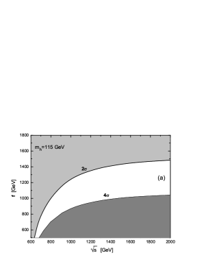
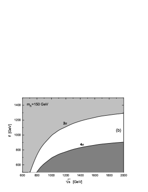
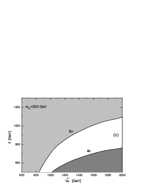
Figure 9: The $LH$ effect observation area(gray) and the $LH$ effect exclusion area (light gray) for the $e^{+}e^{-}\to\gamma\gamma\to t\bar{t}h^{0}$ process in the $\sqrt{s}-f$ parameter space with $c_{\lambda}^{2}=0.8$ and ${\cal L}_{e^{+}e^{-}}=1000~{}fb^{-1}$. (a) is for $m_{h}=115~{}GeV$, (b) is for $m_{h}=150~{}GeV$ and (c) is for $m_{h}=200~{}GeV$.

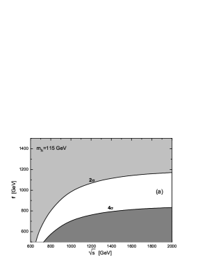
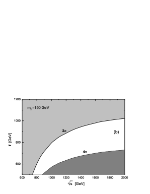
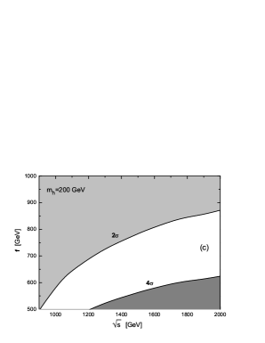
Figure 10: The $LHT$ effect observation area(gray) and the $LHT$ effect exclusion area (light gray) for the $e^{+}e^{-}\to\gamma\gamma\to t\bar{t}h^{0}$ process in the $\sqrt{s}-f$ parameter space with $c_{\lambda}^{2}=0.8$ and ${\cal L}_{e^{+}e^{-}}=1000~{}fb^{-1}$. (a) is for $m_{h}=115~{}GeV$, (b) is for $m_{h}=150~{}GeV$ and (c) is for $m_{h}=200~{}GeV$.

In order to compare the production rates in different polarization cases of initial photons for process $\gamma\gamma\to t\bar{t}h^{0}$ , we depict their cross sections of process $\gamma\gamma\to t\bar{t}h^{0}$ as the functions of the $\gamma\gamma$ colliding energy $\sqrt{\hat{s}}$ in Fig.11(a) and (b) in the frameworks of $LH$ and $LHT$ model separately, where $m_{h}=150~{}GeV$, $f=1~{}TeV$ for the $LH$ model and $f=0.5~{}TeV$ for the $LHT$ model, and the notation of $+~{}-$ represents helicities of the two initial photons being $\lambda_{1}=1$ and $\lambda_{2}=-1$. Since the cross-sections of the $+~{}-$ and $-~{}+$ photon polarization (J=2) are equal, and also the cross-sections of the $+~{}+$ and $-~{}-$ photon polarization (J=0) are the same, we only present the total cross-sections in three cases in Fig.11(a,b): $+~{}-$, $+~{}+$ and unpolarized photons. We can see from the figures that the $LH/LHT$ model effects in the $+~{}+$ photon polarization case are obviously enhanced in comparison with the unpolarized photon case in the vicinity of $\sqrt{\hat{s}}\sim 700~{}GeV$, while the $LH/LHT$ model effects in the $+~{}-$ case are more significant when $1.2~{}TeV<\sqrt{\hat{s}}<1.8~{}TeV$.

In Fig.12(a-b), we plot the distributions of the transverse momenta of the final states($p_{T}^{t}$ and $p_{T}^{h}$) for the process $\gamma\gamma\to t\bar{t}h^{0}$ with $c_{\lambda}^{2}=0.8$, $m_{h}=150~{}GeV$, $\sqrt{\hat{s}}=800~{}GeV$ and $f=1(0.5)~{}TeV$(in the $LH(LHT)$ model) at the ILC. Due to the CP-conservation, the distributions of the transverse momentum of anti-top quark, $p_{T}^{\bar{t}}$, in the process $\gamma\gamma\to t\bar{t}h^{0}$ should be the same as that of $d\sigma_{SM}/dp_{T}^{t}$ shown in Fig12(a). These figures demonstrate that the $LH$ and $LHT$ model corrections significantly modify the $SM$ distributions of the differential cross sections $d\sigma_{SM}/dp_{T}^{t}$ and $d\sigma_{SM}/dp_{T}^{h}$ at the ILC, respectively. We find that in the regions around $p_{T}^{t}\sim 200~{}GeV$ and $p_{T}^{h}\sim 100~{}GeV$, the $LH/LHT$ corrections can be more significant than in other regions.

Figure 11: The cross sections of the process $\gamma\gamma\to t\bar{t}h^{0}$ as the functions of $\gamma\gamma$ c.m.s. energy $\sqrt{\hat{s}}$ when $m_{h}=150~{}GeV$ and $c_{\lambda}^{2}=0.8$. (a) is for the $LH$ model with $f=1~{}TeV$, and (b) is for the $LHT$ model with and $f=0.5~{}TeV$.

Figure 12: The transverse momentum distributions of the final state particles($t,h^{0}$) at QCD NLO for the process $\gamma\gamma\to t\bar{t}h^{0}$ with $c_{\lambda}^{2}=0.8$, $m_{h}=150~{}GeV$, $\sqrt{\hat{s}}=800~{}GeV$ and $f=1(0.5)~{}TeV$(in the $LH(LHT)$ model) at the ILC. (a) is for the distributions of $p_{T}^{t}$, and (b) is for the distributions of $p_{T}^{h}$.

$\sqrt{s}$	$m_{h}$	$LH$:  $f$ [GeV]	$LHT$:  $f$ [GeV]
[TeV]	[GeV]	$2\sigma$,     $4\sigma$	$2\sigma$,     $4\sigma$
	115	1004,     712	803,    578
0.8	150	740,     500	602,    466
	200	467,     390	500,    446
	115	1246,     875	985,    708
1.0	150	991,     688	796,    570
	200	707,     488	592,    462
	115	1429,    1009	1130,    810
1.5	150	1216,      851	966,    692
	200	978,      683	784,    566

Table 1: The dependence of the $2\sigma$ exclusion limits and corresponding $4\sigma$ observation limits on $f$ and $\sqrt{s}$ for the $e^{+}e^{-}\to\gamma\gamma\to t\bar{t}h^{0}$ process with $c_{\lambda}^{2}=0.8$ in the $LH$ and $LHT$ model.

V Summary

We investigated the effects of the littlest models with and without T-parity including the QCD NLO corrections, on the associated $t\bar{t}h^{0}$ production process $e^{+}e^{-}\to\gamma\gamma\to t\bar{t}h^{0}$ at future electron-positron linear colliders. We present the regions of $\sqrt{s}-f$ parameter space in which the $LH$ and $LHT$ effects can and cannot be discovered with the criteria assumed in Eqs. (4.2) and (4.3). The production rates of process $\gamma\gamma\to t\bar{t}h^{0}$ in different incoming photon polarization collision modes are also discussed. We find that the measurement of the process $\gamma\gamma\to t\bar{t}h^{0}$ in polarized photon collision mode is of benefit to discovering the effects of the $LH/LHT$ model in some specific c.m.s. energy ranges. We discover that the effects of the $LHT$ model in the process $e^{+}e^{-}\to\gamma\gamma\to t\bar{t}h^{0}$ generally can be greater than in the $LH$ model when the symmetry breaking scale $f$ has a relative small value due to the $t-\bar{t}-h^{0}$ coupling difference between the $SM$, $LHT$ and the $LH$ model. Our results show that the relative deviation $R_{1}$ for the $LH$ model in the process $e^{+}e^{-}\to\gamma\gamma\to t\bar{t}h^{0}$ is always positive, while $R_{2}$ for the $LHT$ model is negative in our chosen range of the symmetry breaking scale $f$. We conclude that the future experiment at the $ILC$ could discover the effects on the $e^{+}e^{-}\to\gamma\gamma\to t\bar{t}h^{0}$ cross section contributed by the $LH$ or $LHT$ model in some parameter space, or put more stringent constraints on the $LH$/$LHT$ parameters.

Acknowledgments: This work was supported in part by the National Natural Science Foundation of China, the Education Ministry of China and a special fund sponsored by Chinese Academy of Sciences.

References

• [1] S. L. Glashow, Nucl. Phys. 22 (1961) 579; S. Weinberg, Phys. Rev. Lett. 1 (1967) 1264; A. Salam, Proc. 8th Nobel Symposium Stockholm 1968,ed. N. Svartholm (Almquist and Wiksells, Stockholm 1968) p.367; H. D. Politzer, Phys. Rep. 14 (1974) 129.
• [2] P. W. Higgs, Phys. Lett 12 (1964) 132, Phys. Rev. Lett. 13 (1964) 508; Phys. Rev. 145 (1966) 1156; F. Englert and R.Brout, Phys. Rev. Lett. 13 (1964) 321; G. S. Guralnik, C. R. Hagen and T. W. B. Kibble, Phys. Rev. Lett. 13 (1964) 585; T. W. B. Kibble, Phys. Rev. 155 (1967) 1554.
• [3] N. Arkani-Hamed, A.G. Cohen and H. Georgi, Phys. Lett. B513, 232(2001); Phys. Lett. B513, 232(2001); N. Arkani-Hamed, A.G. Cohen, E.Katz, A.E. Nelson, T. Gregoire and J.G. Wacker, JHEP0208, 021(2002); M. Perelstain, Prog. Part. Nucl. Phys. 58 (2007) 247, arXiv:hep-ph/0512128.
• [4] N. Arkani-hamed, A. G. Cohen and H. Georgi, Phys. Lett. B513, (2001)232, arXiv:hep-ph/0105239.
• [5] N. Arkani-hamed, A. G. Cohen, T. Gregoire and J. G.Jacker, JHEP 0208, (2002)020, arXiv:hep-ph/0202089.
• [6] N. Arkani-hamed, A. G. Cohen, E. Katz, A. E. Nelson, T. Gregoire and J. G. Wacker, JHEP 0208(2002) 021, arXiv:hep-ph/0206020.
• [7] I. Low, W. Skiba and D.Smith, Phys. Rev. D66, (2002)072001, arXiv:hep-ph/0207243.
• [8] N. Arkani-hamed, A. G. Cohen, E. Katz and A. E. Nelson, JHEP 0207(2002)304, arXiv:hep-ph/0206021.
• [9] For a recent review, see e.g., M. Schmaltz, Nucl. Phys. Proc. Suppl. 117 40-49 (2003), arXiv:hep-ph/0210415.
• [10] T. Gregoire and J. G. Wacker, JHEP 0208, 019 (2002) arXiv:hep-ph/0206023.
• [11] C. Csaki, J. Hubisz, G.D. Kribs, P. Meade, and J. Terning, Phys. Rev. D67, 115002 (2003)arXiv:hep-ph/0211124; Phys. Rev. D68, 035009 (2003)arXiv:hep-ph/0303236; J. L. Hewett, F. J. Petriello, and T. G. Rizzo, JHEP0310, 062 (2003) arXiv:hep-ph/0211218; Mu-Chun Chen and Sally Dawson, Phys. Rev. D70, 015003 (2004)arXiv:hep-ph/0311032; W. Kilian and J. Reuter, Phys. Rev. D70, 015004 (2004)arXiv:hep-ph/0311095; Zhenyu Han and Witold Skiba, Phys. Rev. D72, 035005 (2005) arXiv:hep-ph/0506206.
• [12] H. C. Cheng and I. Low, JHEP0309, 051 (2003) arXiv:hep-ph/0308199; JHEP0408, 061 (2004) arXiv:hep-ph/0405243. I. Low, JHEP0410, 067 (2004) arXiv:hep-ph/0409025; J. Hubisz, and P. Meade, Phys. Rev. D71, 035016(2005) arXiv:hep-ph/0411264; J. Hubisz, S.J. Lee, and G. Paz, JHEP0606, 041(2006) arXiv:hep-ph/0512169.
• [13] J. Hubisz, P. Meade, A. Noble, et al. JHEP0601, (2006)135;
• [14] T. Han, H.E. Logan, B. McElrath and L.-T. Wang, Phys. Rev. D67 (2003) 095004, arXiv:hep-ph/0301040; T. Han, H.E. Logan, B. McElrath and L.-T. Wang, Phys. Lett. B563 (2003) 191 and Erratum-ibid. Phys. Lett. B603 (2004) 257, arXiv:hep-ph/0302188; T. Han, H.E. Logan, B. McElrath and L.-T. Wang, JHEP0601 (2006) 099, arXiv:hep-ph/0506313.
• [15] A. Belyaev, C.-R. Chen, K.Tobe, C.-P. Yuan, Phys.Rev. D74 (2006) 115020, arXiv:hep-ph/0609179, J. Hubisz and P. Meade, Phys.Rev. D71 (2005) 035016, arXiv:hep-ph/0411264.
• [16] T. Abe et al. [American Linear Collider Working Group Collaboration], ”Linear collider physics resource book for Snowmass 2001”, in Proc. of the APS/DPF/DPB Summer Study on the Future of Particle Physics (Snowmass 2001) arXiv:hep-ex/0106055, arXiv:hep-ex/0106056, arXiv:hep-ex/0106057, arXiv:hep-ex/0106058, and the references therein.
• [17] H. Baer, S. Dawson and L. Reina, Phys. Rev. D61 (1999) 013002.
• [18] J. A. Aguilar-Saavedra et al. [ECFA/DESY LC Physics Working Group Collaboration], β€œTESLA Technical Design Report Part III:Physics at an $e^{+}e^{-}$-Linear Collider”, arXiv:hep-ph/0106315, and the references therein.
• [19] K. Abe et al., [ACFA Linear Collider Working Group Collaboration], ”Particle physics experiments at JLC”, arXiv:hep-ph/0109166, and the references therein.
• [20] M. Battaglia and K. Desch, arXiv:hep-ph/0101165 and references therein.
• [21] Y. You, W.-G. Ma, H. Chen, R.-Y. Zhang, Y.-B. Sun, H.-S. Hou, Phys. Lett. B571(2003)85, arXiv:hep-ph/0306036.
• [22] G. Belanger, F. Boudjema, J. Fujimoto, T. Ishikawa, T. Kaneko, K. Kato, Y. Shimizu and Y. Yasui, Phys. Lett.B571(2003)163, arXiv:hep-ph/0307029.
• [23] A. Denner, S. Dittmaier, M. Roth, M. M. Weber, Phys.Lett.B575(2003)290, arXiv:hep-ph/0307193.
• [24] X.H. Wu, C.S. Li and J.J. Liu, arXiv:hep-ph/0308012.
• [25] Chong-Xing Yue, Wei Wang, Feng Zhang, Commu. Theor. Phys. 45(2006) 511, arXiv:hep-ph/0503260.
• [26] Chong-Xing Yue, Nan Zhang, arXiv:hep-ph/0609247.
• [27] C. Casaki, J. Hubisz, G.D. Kribs, P. Meade and J. Terning, Phy.Rev. D68,(2003) 035009; T. Gregoire, D.R. Smith and J.G. Wacker, Phy.Rev. D69,(2004)115008.
• [28] V.I. Telnov, ”Physics options at the ILC. GG6 summary at Snowmass2005”, physics 0512048; V.I. Telnov, Acta Phys.Polon. B37, 633 (2006), physics 0602172.
• [29] H. Chen, W.-G. Ma, R.-Y. Zhang, P.-J. Zhou, H.-S. Hou and Y.-B. Sun, Nucl. Phys. B683 (2004)196, arXiv:hep-ph/0309106.
• [30] N. Arkani-Hamed, A.G. Cohen, E. Katz, and A.E. Nelson, JHEP0207 (2002) 034 .
• [31] J. Hubisz, P. Meade, Phys. Rev. D71, 035016 (2005); C. R. Chen, K. Tobe, C.-P. Yuan, Phys. Lett. B640, 263 (2006).
• [32] A. Belyaev, C. R. Chen, K. Tobe, C.-P. Yuan, Phys.Rev. D74 (2006) 115020, arXiv:hep-ph/0609179.
• [33] G. Burdman, M. Perelstein and A. Pierce, Phys. Rev. Lett. 90, (2003) 241802 and Erratum-ibid. 92, (2004) 049903, arXiv:hep-ph/0212228; C. Dib, R. Rosenfeld and A. Zerwekh, arXiv:hep-ph/0302068.
• [34] W.-M. Yao, $et$ $al$., J. of Phys. G33, 1 (2006).
• [35] T. Hahn, Comp. Phys. Commun. 140, 418 (2001).
• [36] W. T. Giele and E. W. Glover, Phys. Rev. D46, 1980 (1992); W. T. Giele, E. W. Glover and D. A. Kosower, Nucl. Phys. B403, 633 (1993); S. Keller and E. Laenen, Phys. Rev. D59, 114004 (1999).
• [37] I. Ginzburg, G. Kotkin, V. Serbo and V. Telnov, Pizma ZhETF, 34 (1981) 514; JETP Lett. 34 (1982) 491. Preprint INP 81-50, 1981, Novosibirsk.
• [38] I. Ginzburg, G. Kotkin, V. Serbo and V. Telnov, Nucl. Instr. and Meth. 205 (1983) 47, Preprint INP 81-102, 1991, Novosibirsk.
• [39] I. Ginzburg, G. Kotkin, S. Panfil, V. Serbo and V. Telnov, Nucl. Instr. and Meth. 219 (1984) 5.
• [40] G. Jikia. Nucl. Phys., 1992, B374: 83; O. J. P. Eboli $et$ $al$., Phys. Rev. D47, 1889(1993).
• [41] K. Cheung, Phys.Rev. D47, 3750(1993).