Dispersionless limit of the noncommutative potential KP hierarchy and solutions of the pseudodual chiral model in $2+1$ dimensions

Abstract

The usual dispersionless limit of the KP hierarchy does not work in the case where the dependent variable has values in a noncommutative (e.g. matrix) algebra. Passing over to the potential KP hierarchy, there is a corresponding scaling limit in the noncommutative case, which turns out to be the hierarchy of a “pseudodual chiral model” in $2+1$ dimensions (“pseudodual” to a hierarchy extending Ward’s (modified) integrable chiral model). Applying the scaling procedure to a method generating exact solutions of a matrix (potential) KP hierarchy from solutions of a matrix linear heat hierarchy, leads to a corresponding method that generates exact solutions of the matrix dispersionless potential KP hierarchy, i.e. the pseudodual chiral model hierarchy. We use this result to construct classes of exact solutions of the $su(m)$ pseudodual chiral model in $2+1$ dimensions, including various multiple lump configurations.

1 Introduction

Expressing the scalar KP hierarchy with dependent variable $u(t_{1},t_{2},\ldots)$ in terms of new evolution variables $T_{n}=\epsilon\,t_{n}$ with a parameter $\epsilon$, the limit $\epsilon\to 0$ (keeping $T_{n}$ fixed) leads to the so-called dispersionless KP hierarchy (see [Koda88, Koda+Gibb89, Kupe90qc, Kric92, Zakh94, Aoya+Koda94, Taka+Take95, Taka95, Stra95, Stra97, Chan+Tu00, Wieg+Zabr00, KMR01, DMT01, Duna+Tod02, Kono+Mart02, Kono+Mart02SIAM, MMM02, MMM02b, GMM03, Fera+Khus04, Mana+Sant06, Kono+Magr06], for example). The same limit does not work, however, for the KP hierarchy with dependent variable in a noncommutative (e.g. matrix) algebra. In fact, different scaling limits of the matrix KP equation have already been explored in [Zakh+Kuzn86], where the multiscale expansion method has been used to relate different integrable systems.

In the present work we formulate a dispersionless limit of the “noncommutative” potential KP (ncpKP) hierarchy with dependent variable $\phi$, where $u=\phi_{t_{1}}$. It turns out to be the hierarchy associated with a “pseudodual chiral model” (pdCM) in $2+1$ dimensions, a well-known reduction of the self-dual Yang-Mills equation [Lezn87, Maso+Wood96]. Applying the scaling limit procedure to a method generating exact solutions of a matrix pKP hierarchy from solutions of a matrix linear heat hierarchy, then results in a method generating solutions of this pdCM hierarchy.

In section 2 we consider the dispersionless limit of the ncpKP equation. Section 3 generalizes this limit to the whole ncpKP hierarchy, explores some of its properties, and in particular establishes a pseudoduality relation with a hierarchy that extends Ward’s (modified) chiral model in $2+1$ dimensions [Ward88, Ward88torsion, Ward89, Ward90, Ward94, Ward95]. The latter model has been studied extensively [Lees89, Vill89, Sutc92, Sutc93, PSZ92, Ioan+Ward95, Ioan96, Ioan00, Ioan+Zakr98PLA, Ioan+Zakr98PLA2, Ioan+Zakr98JMP, Ioan+Mant05, Anand97, Anand98, ZMA05, Dai+Tern05, DTU06, Dai+Tern07, Duna+Mant05, Duna+Plan07] (see also [Ward99, Kote+Ward01, Ji+Zhou05] for the Ward model in (anti-) de Sitter space-time and [Lech+Popo01b, Lech+Popo01c, Biel02, Wolf02, Ihl+Uhlm03, Chu+Lech05, Chu+Lech06, KLP06] for explorations of a Moyal-deformed version), in particular concerning its (multi-) lump solutions, which are two-dimensional soliton-like objects. In this respect, its pseudodual received comparatively little attention. The dependent variables of the two equations are related by a kind of hetero-Bäcklund transformation. Given a solution of one of the two equation, this becomes a first order system of partial differential equations, which determines a solution of the other equation. The necessary integration is typically difficult to carry out, however. Hence, although some properties of the pseudodual model can certainly be infered from corresponding knowledge of the Ward model, there is no explicit translation of its solutions. In any case, in this work we present an independent approach to solutions of the pdCM and moreover to its hierarchy.

In section 4 we derive the abovementioned method to generate exact solutions of the pdCM hierarchy from corresponding knowledge of the ncpKP hierarchy. The main result is independently verified in section 5 and then applied to construct some classes of exact solutions. This section is actually formulated in such a way that it can be accessed almost without any knowledge of the previous sections. We concentrate on solutions of the $su(m)$ pdCM hierarchy and restrict concrete examples to the $su(2)$ case. Some conclusions are collected in section 6.

2 The dispersionless limit of the noncommutative pKP equation

Let $\phi(\mathbf{t})$ with $\mathbf{t}=(t_{1},t_{2},\ldots)$ be a function with values in some matrix space $\mathcal{A}$ which is endowed with a product $A\cdot B=AQB$, where $Q$ is a constant matrix, i.e. independent of $\mathbf{t}$. We consider the following ncpKP equation,

$$4\,\phi_{tx}-\phi_{xxxx}-3\,\phi_{yy}=6\,(\phi_{x}Q\phi_{x})_{x}-6\,[\phi_{x},\phi_{y}]_{Q}\,,$$ (2.1)

where $x=t_{1},y=t_{2},t=t_{3}$ and

$$[A,B]_{Q}:=AQB-BQA\;.$$ (2.2)

Let $\phi$ now also depend on a parameter $\epsilon$ in such a way that

$$\phi(\mathbf{t},\epsilon)=\epsilon^{a}\Phi(\mathbf{T})+\mathcal{O}(\epsilon^{a+1})$$ (2.3)

with some integer $a$. Furthermore, we assume that $Q$ has an expansion

$$Q=Q_{(0)}+\epsilon\,Q_{(1)}+\mathcal{O}(\epsilon^{2})\;.$$ (2.4)

Rewriting the ncpKP equation in terms of the rescaled variables $T_{n}=\epsilon\,t_{n}$, dividing the equation by the maximal power of $\epsilon$ common to all of its summands, and taking the limit $\epsilon\to 0$ while keeping $T_{1},T_{2},\ldots$ fixed, should result in an equation that still has linear as well as nonlinear terms (in $\Phi$). This fixes the value of $a$, but we have to distinguish the following two cases.

If the algebra $(\mathcal{A},\cdot)$ is commutative at $\epsilon=0$ with $Q_{(0)}\neq 0$, and hence the commutator $[\Phi_{X},\Phi_{Y}]_{Q_{(0)}}=\Phi_{X}Q_{(0)}\Phi_{Y}-\Phi_{Y}Q_{(0)}\Phi_{X}$ vanishes, then our requirements lead to $a=-1$, and the scaling limit of the pKP equation, divided by $\epsilon$, is

$$4\,\Phi_{TX}-3\,\Phi_{YY}=6\,(\Phi_{X}Q_{(0)}\Phi_{X})_{X}-6\,[\Phi_{X},\Phi_{Y}]_{Q_{(1)}}\,,$$ (2.5)

where $X=T_{1},Y=T_{2},T=T_{3}$. If $\Phi$ is a scalar and $Q_{(0)}=1$, the last equation reduces to

$$4\,\Phi_{TX}-3\,\Phi_{YY}=6\,(\Phi_{X}{}^{2})_{X}\;.$$ (2.6)

This is the potential form of the dispersionless limit of the (“commutative”) scalar KP equation, which is also known as the Khokhlov-Zabolotskaya equation (see [Kric92] for instance).

If the algebra $(\mathcal{A},\cdot)$ is noncommutative at $\epsilon=0$, we have to set

$$a=0\,,$$ (2.7)

and this choice will be made throughout this work. Then we obtain the following dispersionless limit of the ncpKP equation (2.1),

$$4\,\Phi_{TX}-3\,\Phi_{YY}=-6\,[\Phi_{X},\Phi_{Y}]_{Q_{(0)}}\;.$$ (2.8)

Up to the modified matrix product and rescalings of the coordinates, this is a well-known reduction of the self-dual Yang-Mills equation (see [Lezn87, Lezn+Mukh87, Lezn+Save89, Papa89, Papa91recur, Maso+Wood96, Foka+Ioan01]). With the further dimensional reduction $\Phi_{X}=\Phi_{T}$, it becomes the pseudodual chiral model [Frad+Tsey85, Curt+Zach94, Curt+Zach95para] (see also [Zakh+Mikh78rel, Napp80, Frid+Jevi84, Lezn+Mukh87]). Accordingly, we may call (2.8) a pseudodual chiral model in $2+1$ dimensions, in the following abbreviated to pdCM. In fact, as explained in section 3.2, it is “pseudodual” to an integrable (modified) chiral model in $2+1$ dimensions.

3 The dispersionless limit of the ncpKP hierarchy

A functional representation of the ncpKP hierarchy is given by [DMH07Burgers]

$$(\phi-\phi_{-[\lambda]})(\lambda^{-1}-Q\phi)-\phi_{t_{1}}=\theta-\theta_{-[\lambda]}\,,$$ (3.9)

where $\theta$ is an arbitrary $\mathcal{A}$-valued function, and $(\phi_{-[\lambda]})(\mathbf{t}):=\phi(\mathbf{t}-[\lambda])$ is a Miwa shift with $[\lambda]=(\lambda,\lambda^{2}/2,\lambda^{3}/3,\ldots)$, $\lambda$ an indeterminate. Eliminating $\theta$ from this equation, we get the following functional form of the ncpKP hierarchy,

$$\Big{(}(\phi-\phi_{-[\lambda]})(\lambda^{-1}-Q\phi)-\phi_{t_{1}}\Big{)}-\Big{(}(\phi-\phi_{-[\lambda]})(\lambda^{-1}-Q\phi)-\phi_{t_{1}}\Big{)}_{-[\mu]}$$ (3.10)

$$= \Big{(}(\phi-\phi_{-[\mu]})(\mu^{-1}-Q\phi)-\phi_{t_{1}}\Big{)}-\Big{(}(\phi-\phi_{-[\mu]})(\mu^{-1}-Q\phi)-\phi_{t_{1}}\Big{)}_{-[\lambda]}\,,$$

where $\mu$ is another indeterminate.

If $\mathbf{p}_{n}$, $n=1,2,\ldots$, denote the elementary Schur polynomials, then

$$\mathbf{p}_{n}(-\tilde{\partial})=-\frac{\epsilon}{n}\,\partial_{T_{n}}+\mathcal{O}(\epsilon^{2})\,,$$ (3.11)

where $\tilde{\partial}=(\partial_{t_{1}},\partial_{t_{2}}/2,\partial_{t_{3}}/3,\ldots)$, and hence

$$\phi-\phi_{-[\lambda]}=\epsilon\,D(\lambda)\Phi+\mathcal{O}(\epsilon^{2})\,,$$ (3.12)

where

$$D(\lambda):=\sum_{n\geq 1}{\lambda^{n}\over n}\,\partial_{T_{n}}\;.$$ (3.13)

In accordance with (2.3), where now $a=0$, we shall assume

$$\theta(\mathbf{t},\epsilon)=\Theta(\mathbf{T})+\mathcal{O}(\epsilon)\;.$$ (3.14)

Then we obtain

$$D(\lambda)(\Phi)\,(\lambda^{-1}-Q_{(0)}\Phi)-\Phi_{T_{1}}=D(\lambda)(\Theta)\;.$$ (3.15)

Expanding this in powers of $\lambda$, we find

$${1\over n+1}\Phi_{T_{n+1}}-{1\over n}\Phi_{T_{n}}Q_{(0)}\Phi={1\over n}\Theta_{T_{n}}\qquad n=1,2\ldots\;.$$ (3.16)

Elimination of $\Theta$ results in the hierarchy equations

$${n\over(n+1)}\Phi_{T_{n+1},T_{m}}-{m\over(m+1)}\Phi_{T_{m+1},T_{n}}=\Phi_{T_{n}}Q_{(0)}\Phi_{T_{m}}-\Phi_{T_{m}}Q_{(0)}\Phi_{T_{n}}\;.$$ (3.17)

Introducing

$$x_{n}:=n\,T_{n}\qquad\quad n=1,2,\ldots\,,$$ (3.18)

this becomes

$$\Phi_{x_{n+1},x_{m}}-\Phi_{x_{m+1},x_{n}}=[\Phi_{x_{n}},\Phi_{x_{m}}]_{Q_{(0)}}\qquad\quad m,n=1,2,\ldots\;.$$ (3.19)

For $m=1,n=2$, we recover (2.8).

Expressing $Q_{(0)}$ as

$$Q_{(0)}=VU^{\dagger}$$ (3.20)

with matrices $U,V$ and the adjoint (complex conjugate and transpose) $U^{\dagger}$ of $U$, then

$$\varphi:=U^{\dagger}\Phi V$$ (3.21)

(which includes the cases $\varphi=Q_{(0)}\Phi$ and $\varphi=\Phi Q_{(0)}$) solves

$$\varphi_{x_{n+1},x_{m}}-\varphi_{x_{m+1},x_{n}}=[\varphi_{x_{n}},\varphi_{x_{m}}]\qquad\quad m,n=1,2,\ldots\,,$$ (3.22)

if $\Phi$ solves (3.19). The power of this observation lies in the fact that any solution of (3.19) in some $M\times N$ matrix algebra, where $Q_{(0)}=VU^{\dagger}$ with an $M\times m$ matrix $U$ and an $N\times m$ matrix $V$, determines in this way a solution of (3.22) in the $m\times m$ matrix algebra. For example, if we are looking for solutions of (3.22) in the algebra of $2\times 2$ matrices, we may first look for solutions of (3.19) with any $M,N\geq 2$ and $Q_{(0)}=VU^{\dagger}$ with $M\times 2$ and $N\times 2$ matrices $U$ and $V$. In this way (simple) solutions of (3.19) in arbitrarily large matrix algebras lead to (complicated) solutions of (3.22) in the algebra of $2\times 2$ matrices. In particular, this explains the significance of $Q_{(0)}$ in our previous formulae. In section 5 we will substantiate this method. The hierarchy (3.22) is consistent with restricting $\varphi$ to take values in any Lie algebra, e.g. $sl(N,\mathbb{R})$, $sl(N,\mathbb{C})$, $u(N)$ or $su(N)$. If $\varphi$ solves (3.22), then also $\varphi+\varphi_{0}$, where $\varphi_{0}$ is a constant in the respective Lie algebra.

As a consequence of their origin, the hierarchies (3.19) and (3.22) are invariant under the scaling transformation $x_{n}\mapsto\lambda\,x_{n}$, $n=1,2,\ldots$, with any constant $\lambda\neq 0$.

Remark. If $g_{1},g_{2}$ are any two constant invertible matrices with size such that $g_{1}\Phi g_{2}$ is defined, then

$$\Phi\mapsto g_{1}\Phi g_{2}\,,\qquad Q_{(0)}\mapsto g_{2}^{-1}Q_{(0)}g_{1}^{-1}$$ (3.23)

leaves (3.19) invariant. If $Q_{(0)}$ is given by (3.20), the latter transformation results from

$$V\mapsto g_{2}^{-1}V\,,\qquad U\mapsto(g_{1}^{\dagger})^{-1}U\,,$$ (3.24)

and $\varphi$ is invariant. More generally, the transformation $V\mapsto g_{2}^{-1}V\sigma$, $U\mapsto(g_{1}^{\dagger})^{-1}U(\sigma^{\dagger})^{-1}$, with a constant $m\times m$ matrix $\sigma$, leads to $\varphi\mapsto\sigma^{-1}\varphi\sigma$. This leaves the hierarchy equations (3.22) invariant. $\square$

3.1 Some properties of the first dispersionless hierarchy equation

A Lagrangian for the first equation ($m=1,n=2$)

$$\varphi_{x_{1},x_{3}}-\varphi_{x_{2},x_{2}}=-[\varphi_{x_{1}},\varphi_{x_{2}}]$$ (3.25)

of the hierarchy (3.22) is

$$\mathcal{L}=-\mathrm{tr}\Big{(}\varphi_{x_{1}}\varphi_{x_{3}}-\varphi_{x_{2}}{}^{2}-{2\over 3}\varphi[\varphi_{x_{1}},\varphi_{x_{2}}]\Big{)}$$ (3.26)

(see also [Lezn+Mukh87, Lezn+Save89]). After passage to the new coordinates $x,y,t$ given by

$$x_{1}=\frac{1}{2}(t-x)\,,\qquad x_{2}=y\,,\qquad x_{3}=\frac{1}{2}(t+x)\,,$$ (3.27)

equation (3.25) becomes

$$\varphi_{tt}-\varphi_{xx}-\varphi_{yy}+[\varphi_{t}-\varphi_{x},\varphi_{y}]=0\,,$$ (3.28)

and the Lagrangian takes the form

$$\mathcal{L}=-\frac{1}{2}\mathrm{tr}\Big{(}\varphi_{t}{}^{2}-\varphi_{x}{}^{2}-\varphi_{y}{}^{2}-{2\over 3}\varphi[\varphi_{t}-\varphi_{x},\varphi_{y}]\Big{)}$$

$$=-\frac{1}{2}\mathrm{tr}\Big{(}\eta^{\mu\nu}\partial_{\mu}\varphi\,\partial_{\nu}\varphi+\frac{2}{3}\varphi\,v_{\rho}\epsilon^{\rho\mu\nu}\partial_{\mu}\varphi\,\partial_{\nu}\varphi\Big{)}\,,$$ (3.29)

where we introduced the components $\eta^{\mu\nu}$ (with respect to the coordinates $(x^{\mu})=(t,x,y)$) of the Minkowski metric in $2+1$ dimensions, the totally antisymmetric Levi-Civita pseudo-tensor with $\epsilon^{012}=1$, and a constant covector $v_{\rho}$ with components $(1,1,0)$. As a consequence of the translational invariance of the Lagrangian, the energy-momentum tensor

$$T^{\mu}{}_{\nu}=\mathrm{tr}\Big{(}\frac{\partial\mathcal{L}}{\partial(\partial_{\mu}\varphi)}\,\partial_{\nu}\varphi-\delta^{\mu}_{\nu}\,\mathcal{L}\Big{)}$$ (3.30)

provides us with the conserved densities

$$T^{0}{}_{0}=-\frac{1}{2}\mathrm{tr}\Big{(}\varphi_{t}^{2}+\varphi_{x}^{2}+\varphi_{y}^{2}-\frac{2}{3}\varphi[\varphi_{x},\varphi_{y}]\Big{)}\,,$$ (3.31)

$$T^{0}{}_{1}=-\mathrm{tr}\Big{(}\varphi_{t}\varphi_{x}-\frac{1}{3}\varphi[\varphi_{x},\varphi_{y}]\Big{)}\,,\qquad T^{0}{}_{2}=-\mathrm{tr}(\varphi_{t}\varphi_{y})\;.$$ (3.32)

Then also

$$\mathcal{E}=T^{0}{}_{0}-T^{0}{}_{1}=-{1\over 2}\mathrm{tr}[(\varphi_{t}-\varphi_{x})^{2}+\varphi_{y}{}^{2}]$$ (3.33)

is a conserved density. For any non-zero anti-Hermitian matrix, the trace of the square of the matrix is real and negative. Hence $\mathcal{E}$ provides us with a non-negative “energy” density in the case where $\varphi$ takes values in the Lie algebra $u(m)$ of the unitary group.

For any infinitesimal symmetry $\delta\varphi=\frac{\partial\varphi}{\partial\alpha}\delta\alpha$ (with a parameter $\alpha$) of the Lagrangian, there is a conserved current

$$J^{\mu}:=\mathrm{tr}\Big{(}\frac{\partial\mathcal{L}}{\partial(\partial_{\mu}\varphi)}\frac{\partial\varphi}{\partial\alpha}\Big{)}\,,$$ (3.34)

i.e., $\partial_{\mu}J^{\mu}=0$. A symmetry of the above Lagrangian is given by $\delta\varphi=[C,\varphi]\alpha$ with any constant (anti-Hermitian) matrix $C$. Hence

$$J^{0}_{C}=-\mathrm{tr}\left(\Big{(}[\varphi,\varphi_{t}]+\frac{1}{3}(\varphi^{2}\varphi_{y}-2\varphi\varphi_{y}\varphi+\varphi_{y}\varphi^{2})\Big{)}\,C\right)$$ (3.35)

is a conserved density.

3.2 Relation with Ward’s chiral model in $2+1$ dimensions

The hierarchy (3.22) is related to the hierarchy of an integrable (modified) chiral model in $2+1$ dimensions. First we note that (3.22) is the integrability condition of the linear system

$$J_{x_{n+1}}=-J\,\varphi_{x_{n}}\qquad\quad n=1,2,\ldots$$ (3.36)

with some invertible $J$. Rewriting this as

$$\varphi_{x_{n}}=-J^{-1}J_{x_{n+1}}\qquad\quad n=1,2,\ldots\,,$$ (3.37)

we find that (3.22) is automatically satisfied and the integrability conditions now take the form

$$(J^{-1}J_{x_{n+1}})_{x_{m}}-(J^{-1}J_{x_{m+1}})_{x_{n}}=0\qquad\quad m,n=1,2,\ldots\,\;.$$ (3.38)

In conclusion, solutions $J$ of (3.38) are in correspondence with solutions $\varphi$ of (3.22) via (3.37). This correspondence is of a nonlocal nature. In particular, given a solution $\varphi$ of (3.22), (3.37) does not directly determine $J^{-1}J_{x_{1}}$. We first have to solve (3.36) for $J$ in order to be able to calculate this expression.

(3.38) is immediately recognized as the dispersionless limit of the noncommutative modified KP hierarchy (see equation (4.12) in [DMH06func]).

For $m=1$ and $n=2$, (3.38) reads

$$(J^{-1}J_{x_{3}})_{x_{1}}-(J^{-1}J_{x_{2}})_{x_{2}}=0\;.$$ (3.39)

This equation apparently first appeared in [Pohl80, Mana+Zakh81]. It is a reduction of the self-dual Yang-Mills equation (see [Pohl80, Lezn+Save89, Maso+Wood96], for example). In terms of the coordinates $x,y,t$ given by (3.27), it takes the form

$$(J^{-1}J_{t})_{t}-(J^{-1}J_{x})_{x}-(J^{-1}J_{y})_{y}+[J^{-1}J_{x},J^{-1}J_{t}]=0\,,$$ (3.40)

or in tensor notation (using the summation convention)

$$(\eta^{\mu\nu}+\epsilon^{\mu\nu})\partial_{\mu}(J^{-1}\partial_{\nu}J)=0\,,$$ (3.41)

where $\mu,\nu=0,1,2$, $(\eta^{\mu\nu})=\mathrm{diag}(1,-1,-1)$, and $\epsilon^{\mu\nu}$ is antisymmetric with $\epsilon^{01}=-\epsilon^{10}=1$ and zero otherwise. We note that the bivector $\epsilon^{\mu\nu}$ breaks Lorentz invariance in $2+1$ dimensions. Using the Lorentz invariant Levi-Civita pseudo-tensor and the constant unit covector $v_{\alpha}$ with components $(0,0,1)$, it can be expressed as $\epsilon^{\mu\nu}=v_{\alpha}\epsilon^{\alpha\mu\nu}$. Another integrable equation is obtained if we choose $v_{\alpha}$ to be timelike [Mana+Zakh81, Ward88, Ioan+Ward95]. (3.41) is Ward’s $(2+1)$-dimensional generalization of the chiral (or sigma) model [Ward88, Ward88torsion, Ward89, Ward90, Ward94, Ward95], see also [Lees89, Vill89, Sutc92, Sutc93, PSZ92, Ioan+Ward95, Ioan96, Ioan00, Ioan+Zakr98PLA, Ioan+Zakr98PLA2, Ioan+Zakr98JMP, Foka+Ioan01, Ioan+Mant05, Anand97, Anand98, ZMA05, Dai+Tern05, Dai+Tern07, Duna+Mant05, Duna+Plan07]. $J$ can be consistently restricted to any Lie group, e.g. $SL(N,\mathbb{R})$, $SL(N,\mathbb{C})$, $U(N)$ or $SU(N)$.

Remark. According to (3.37) we have $J^{-1}J_{y}=\varphi_{x}-\varphi_{t}$ and $J^{-1}J_{t}+J^{-1}J_{x}=-\varphi_{y}$, in terms of the variables $x,y,t$ given by (3.27). Hence

$$\mathcal{E}=\mathcal{E}_{\mathrm{Ward}}-\mathrm{tr}\left(J^{-1}J_{t}\,J^{-1}J_{x}\right)\,,$$ (3.42)

where

$$\mathcal{E}_{\mathrm{Ward}}=-\frac{1}{2}\mathrm{tr}\left((J^{-1}J_{t})^{2}+(J^{-1}J_{x})^{2}+(J^{-1}J_{y})^{2}\right)$$ (3.43)

is the energy density of Ward’s chiral model. The difference between $\mathcal{E}_{\mathrm{Ward}}$ and $\mathcal{E}$ is not a local expression in terms of $\varphi$. The appendix attempts to further clarify the relation between Ward’s chiral model and the pdCM hierarchy (and yet another version of it). $\square$

3.3 An associated bidifferential calculus

On the algebra $\mathcal{A}$ of $m\times m$ matrices with entries depending smoothly on $x_{1},x_{2},\ldots$, we introduce two linear maps $\mathrm{d},\bar{\mathrm{d}}$ by

$$\mathrm{d}\psi=\sum_{n\geq 1}\psi_{x_{n}}\,\mathrm{d}x_{n}\,,\qquad\bar{\mathrm{d}}\psi=\sum_{n\geq 1}\psi_{x_{n+1}}\,\mathrm{d}x_{n}\;.$$ (3.44)

By use of the graded Leibniz rule they extend to a (bi-) differential graded algebra and satisfy

$$\mathrm{d}^{2}=\bar{\mathrm{d}}^{2}=\mathrm{d}\bar{\mathrm{d}}+\bar{\mathrm{d}}\mathrm{d}=0\,,$$ (3.45)

and hence we have a bidifferential calculus. Dressing $\bar{\mathrm{d}}$ by setting

$$\bar{\mathrm{D}}\psi=\bar{\mathrm{d}}\psi-A\,\psi\,,$$ (3.46)

with a 1-form $A=\sum_{n\geq 1}A_{n+1}\mathrm{d}x_{n}$, we find that $\mathrm{d},\bar{\mathrm{D}}$ yields again a bidifferential calculus ($\bar{\mathrm{D}}^{2}=\mathrm{d}\bar{\mathrm{D}}+\bar{\mathrm{D}}\mathrm{d}=0$), iff

$$\mathrm{d}A=0\,,\qquad\bar{\mathrm{d}}A=A\wedge A$$ (3.47)

(see also [DMH00a]). These equations cover Ward’s chiral model hierarchy as well as its pseudodual, which is the dispersionless ncpKP hierarchy. Indeed, solving the first equation by setting

$$A=\mathrm{d}\varphi\,,$$ (3.48)

the second reproduces the pdCM hierarchy

$$\bar{\mathrm{d}}\mathrm{d}\varphi=\mathrm{d}\varphi\wedge\mathrm{d}\varphi\;.$$ (3.49)

Alternatively, solving the second of equations (3.47) by setting

$$A=-J^{-1}\bar{\mathrm{d}}J\,,$$ (3.50)

we recover the hierarchy

$$\mathrm{d}(J^{-1}\bar{\mathrm{d}}J)=0$$ (3.51)

associated with Ward’s chiral model. The relation between both hierarchies is given by

$$J^{-1}\bar{\mathrm{d}}J=-\mathrm{d}\varphi$$ (3.52)

(which is (3.37)). This may be regarded as a “Miura transformation”. The linear system associated with the bidifferential calculus is

$$\bar{\mathrm{D}}\psi-\lambda\,\mathrm{d}\psi=0\,,$$ (3.53)

with a parameter $\lambda$. Taking components of the differential forms, this reads

$$(\partial_{x_{n+1}}-A_{n+1}-\lambda\partial_{x_{n}})\psi=0\qquad\quad n=1,2,\ldots\;.$$ (3.54)

The integrability conditions now have the form

$$[\partial_{x_{n+1}}-A_{n+1}-\lambda\partial_{x_{n}},\partial_{x_{m+1}}-A_{m+1}-\lambda\partial_{x_{m}}]=0\;.$$ (3.55)

Its multicomponent version (and with $m,n\in\mathbb{Z}$) appeared in [Taka90] (see (2.1), (2.2), and also the references therein).

Nonlocal conserved currents are obtained in the following way [DMH00a]. Let $\mathrm{d}\chi_{0}=0$. As a consequence of the bidifferential calculus structure, there are $\chi_{n}$, $n=1,2,\ldots$, such that

$$j_{n+1}:=\bar{\mathrm{D}}\chi_{n}=-\mathrm{d}\chi_{n+1}\qquad\quad n=0,1,\ldots$$ (3.56)

iteratively determines $\chi_{n}$, $n=1,2,\ldots$. For example, starting with $\chi_{0}=\mathcal{I}$ (the unit matrix), we get $j_{1}=\bar{\mathrm{D}}\mathcal{I}=-\mathrm{d}\varphi$ (using (3.48)), hence $\chi_{1}=\varphi+a$ with $\mathrm{d}a=0$, and thus also $\bar{\mathrm{d}}a=0$. In the second step we have $j_{2}=\bar{\mathrm{D}}(\varphi+a)=\bar{\mathrm{d}}\varphi-\mathrm{d}\varphi\,(\varphi+a)$, and the construction of the next current requires the integration of $\mathrm{d}\chi_{2}=\mathrm{d}\varphi\,(\varphi+a)-\bar{\mathrm{d}}\varphi$. The constant $a$ actually turns out to be redundant and should be set to zero.

A Bäcklund transformation is obtained from

$$(\mathrm{d}-\lambda^{-1}\bar{\mathrm{D}})(\mathcal{I}+\lambda^{-1}\mathcal{B})=(\mathcal{I}+\lambda^{-1}\mathcal{B})(\mathrm{d}-\lambda^{-1}\bar{\mathrm{D}}^{\prime})\,,\quad\bar{\mathrm{D}}^{\prime}=\bar{\mathrm{d}}-A^{\prime}\,,$$ (3.57)

with an operator $\mathcal{B}$ (see [DMH01bt]). Expanding in powers of $\lambda^{-1}$, we find

$$[\mathrm{d},\mathcal{B}]=\bar{\mathrm{D}}-\bar{\mathrm{D}}^{\prime}\,,\qquad\bar{\mathrm{D}}\mathcal{B}=\mathcal{B}\bar{\mathrm{D}}^{\prime}\;.$$ (3.58)

Assuming $\mathcal{B}(\psi)=B\psi$ with a matrix $B$, this means

$$\mathrm{d}(B)=A^{\prime}-A\,,\qquad\bar{\mathrm{d}}(B)=AB-BA^{\prime}\;.$$ (3.59)

Using (3.48) and solving the first of these equations by setting $B=\varphi^{\prime}-\varphi-a$ with $\mathrm{d}a=0$, we obtain from the second

$$\bar{\mathrm{d}}(\varphi^{\prime}-\varphi)=\mathrm{d}\varphi\,(\varphi^{\prime}-\varphi-a)-(\varphi^{\prime}-\varphi-a)\,\mathrm{d}\varphi^{\prime}\,,$$ (3.60)

a Bäcklund transformation of the pdCM hierarchy. Alternatively, using (3.50) and solving the second of equations (3.59) by setting $B=-J^{-1}\mathcal{K}J^{\prime}$ with $\bar{\mathrm{d}}\mathcal{K}=0$, the first becomes

$$J^{\prime}{}^{-1}\bar{\mathrm{d}}J^{\prime}-J^{-1}\bar{\mathrm{d}}J=\mathrm{d}(J^{-1}\mathcal{K}J^{\prime})\,,$$ (3.61)

a Bäcklund transformation of the (modified) chiral model hierarchy (see also [OPSC80] for the case of the chiral model on a two-dimensional space-time).

If $\mathcal{B}_{ij}$ leads from an $i$th to a $j$th solution, a permutability relation is given by

$$B_{12}+B_{24}=B_{13}+B_{34}\,,\qquad B_{12}\,B_{24}=B_{13}\,B_{34}$$ (3.62)

(see [DMH01bt]). This determines algebraically a forth solution from a given (first) solution and two Bäcklund descendants of it (with different parameters).

4 Toward exact solutions of the dispersionless ncpKP hierarchy

In this section we start with a result that determines a large class of exact solutions of an ncpKP hierarchy and use the scaling limit toward the dispersionless hierarchy in order to obtain from it a corresponding result that determines exact solutions of the latter, which is a pdCM hierarchy. Let us recall theorem 4.1 from [DMH07Burgers].

Theorem 1

Let $(\mathcal{A},\cdot)$ be the algebra of $M\times N$ matrices of functions of $\mathbf{t}$ with the product

$$A\cdot B=AQB\,,$$ (4.63)

where the ordinary matrix product is used on the right hand side, and $Q$ is a constant $N\times M$ matrix. Let $\tilde{\mathcal{X}}$ be an invertible $N\times N$ matrix and $\tilde{\mathcal{Y}}\in\mathcal{A}$, such that $\tilde{\mathcal{X}},\tilde{\mathcal{Y}}$ solve the linear heat hierarchy (i.e. $\partial_{t_{n}}(\tilde{\mathcal{X}})=\partial_{t_{1}}^{n}(\tilde{\mathcal{X}})$, $n=2,3,\ldots$, and correspondingly for $\tilde{\mathcal{Y}}$) and satisfy

$$\tilde{\mathcal{X}}_{t_{1}}=R\,\tilde{\mathcal{X}}+Q\,\tilde{\mathcal{Y}}\,,$$ (4.64)

with a constant $N\times N$ matrix $R$. The pKP hierarchy in $(\mathcal{A},\cdot)$ is then solved by

$$\phi:=\tilde{\mathcal{Y}}\,\tilde{\mathcal{X}}^{-1}\;.$$ (4.65)

$\square$

A functional representation of the heat hierarchy condition is

$$\lambda^{-1}(\tilde{\mathcal{X}}-\tilde{\mathcal{X}}_{-[\lambda]})=\tilde{\mathcal{X}}_{t_{1}}\,,$$ (4.66)

and correspondingly for $\tilde{\mathcal{Y}}$ (with an indeterminate $\lambda$). The theorem provides us with a method to construct exact solutions of the ncpKP hierarchy in $(\mathcal{A},\cdot)$. The idea is now to take the dispersionless limit of (4.64) and (4.66). This should then result in conditions that determine exact solutions of the pdCM hierarchy in $(\mathcal{A},\cdot)$. However, assuming for $\tilde{\mathcal{X}},\tilde{\mathcal{Y}}$ power series expansions in $\epsilon$ with nonvanishing terms of zeroth order, this results in too restrictive conditions. The way out is to note that a “gauge transformation”

$$\tilde{\mathcal{X}}=\mathcal{X}\,G\,,\qquad\tilde{\mathcal{Y}}=\mathcal{Y}\,G\,,$$ (4.67)

with an $N\times N$ matrix $G$, leaves $\phi$ invariant. Choosing

$$G=\exp(\xi(\mathbf{t},P))\,,\qquad\xi(\mathbf{t},P):=\sum_{n\geq 1}t_{n}\,P^{n}\,,$$ (4.68)

with a constant $N\times N$ matrix $P$, and using $\xi(\mathbf{t},P)_{-[\lambda]}=\xi(\mathbf{t},P)+\ln(\mathcal{I}_{N}-\lambda P)$ with the $N\times N$ unit matrix $\mathcal{I}_{N}$, the heat hierarchy equations are mapped to

$$(\mathcal{X}-\mathcal{X}_{-[\lambda]})(\lambda^{-1}-P)=\mathcal{X}_{t_{1}}\,,\quad(\mathcal{Y}-\mathcal{Y}_{-[\lambda]})(\lambda^{-1}-P)=\mathcal{Y}_{t_{1}}\,,$$ (4.69)

and (4.64) is converted into

$$\mathcal{X}_{t_{1}}+\mathcal{X}P=R\mathcal{X}+Q\mathcal{Y}\;.$$ (4.70)

Assuming that

$$\mathcal{X}(\mathbf{t},\epsilon)=\mathcal{X}_{(0)}(\mathbf{T})+\mathcal{O}(\epsilon)\,,\quad\mathcal{Y}(\mathbf{t},\epsilon)=\mathcal{Y}_{(0)}(\mathbf{T})+\mathcal{O}(\epsilon)\,,$$ (4.71)

$$R=R_{(0)}+\mathcal{O}(\epsilon)\,,\quad Q=Q_{(0)}+\mathcal{O}(\epsilon)\,,$$ (4.72)

and $P$ independent of $\epsilon$, then we obtain from (4.70)

$$\epsilon\mathcal{X}_{(0),T_{1}}+\mathcal{X}_{(0)}P=R_{(0)}\mathcal{X}_{(0)}+Q_{(0)}\mathcal{Y}_{(0)}+\mathcal{O}(\epsilon)\,,$$ (4.73)

and from (4.69)

$$\epsilon\,D(\lambda)\mathcal{X}_{(0)}\,(\lambda^{-1}-P)=\epsilon\mathcal{X}_{(0),T_{1}}+O(\epsilon^{2})\,,$$ (4.74)

together with the same equation for $\mathcal{Y}_{(0)}$. After dividing the last equation by $\epsilon$, these equations have the dispersionless limits

$$R_{(0)}\mathcal{X}_{(0)}+Q_{(0)}\mathcal{Y}_{(0)}=\mathcal{X}_{(0)}P\,,$$ (4.75)

respectively

$$D(\lambda)\mathcal{X}_{(0)}\,(\lambda^{-1}-P)=\mathcal{X}_{(0),T_{1}}\,,\quad D(\lambda)\mathcal{Y}_{(0)}\,(\lambda^{-1}-P)=\mathcal{Y}_{(0),T_{1}}\,,$$ (4.76)

which is

$$\frac{1}{n+1}\mathcal{X}_{(0),T_{n+1}}=\frac{1}{n}\mathcal{X}_{(0),T_{n}}P\,,\quad\frac{1}{n+1}\mathcal{Y}_{(0),T_{n+1}}=\frac{1}{n}\mathcal{Y}_{(0),T_{n}}P\,,$$ (4.77)

($n=1,2,\ldots$), or in terms of the variables (3.18),

$$\mathcal{X}_{(0),x_{n+1}}=\mathcal{X}_{(0),x_{n}}P\,,\quad\mathcal{Y}_{(0),x_{n+1}}=\mathcal{Y}_{(0),x_{n}}P\,,\quad\quad n=1,2,\ldots\;.$$ (4.78)

Under the stated conditions, we have an expansion

$$\phi(\mathbf{t},\epsilon)=\Phi(x_{1},x_{2},\ldots)+\mathcal{O}(\epsilon)\,,$$ (4.79)

which determines an exact solution $\Phi$ of the dispersionless limit of the ncpKP hierarchy, i.e. the pdCM hierarchy (3.19). Proposition 1 in the following section confirms this directly, i.e. without reference to the scaling limit procedure applied to the ncpKP hierarchy and the above theorem.

5 Exact solutions of the pdCM hierarchy

The main result of the preceding section will be formulated in the next proposition, and we provide a direct proof. It will then be further elaborated and applied in order to construct some classes of exact solutions of the ($su(m)$) pdCM hierarchy. In this section, symbols like $\mathcal{X}$ and $Q$, for example, correspond to $\mathcal{X}_{(0)}$ and $Q_{(0)}$ in the preceding sections. Since now we resolve our considerations from the dispersionless limit procedure, there is no need to carry these indices with us any more. In fact, this section can be accessed almost completely without reference to the previous ones.

Proposition 1

Let $\mathcal{X}$ be an invertible $N\times N$ and $\mathcal{Y}$ an $M\times N$ matrix such that

$$R\mathcal{X}+Q\mathcal{Y}=\mathcal{X}P$$ (5.80)

and

$$\mathcal{X}_{x_{n+1}}=\mathcal{X}_{x_{1}}P^{n}\,,\quad\mathcal{Y}_{x_{n+1}}=\mathcal{Y}_{x_{1}}P^{n}\,,\qquad n=1,2,\ldots\,,$$ (5.81)

with constant matrices $P,R$ of size $N\times N$, and $Q$ of size $N\times M$. Then

$$\Phi=\mathcal{Y}\mathcal{X}^{-1}$$ (5.82)

solves the pdCM hierarchy

$$\Phi_{x_{n+1},x_{m}}-\Phi_{x_{m+1},x_{n}}=[\Phi_{x_{n}},\Phi_{x_{m}}]_{Q}\qquad\quad m,n=1,2,\ldots$$ (5.83)

(which is (3.19) with $Q_{(0)}$ replaced by $Q$).

Proof: (5.81) is equivalent to

$$\mathcal{X}_{x_{n+1}}=\mathcal{X}_{x_{n}}P\,,\quad\mathcal{Y}_{x_{n+1}}=\mathcal{Y}_{x_{n}}P\,,\qquad n=1,2,\ldots\;.$$

In terms of the maps $\mathrm{d},\bar{\mathrm{d}}$, defined in section 3.3, this can be expressed as

$$\bar{\mathrm{d}}\mathcal{X}=\mathrm{d}\mathcal{X}\,P\,,\qquad\bar{\mathrm{d}}\mathcal{Y}=\mathrm{d}\mathcal{Y}\,P\;.$$

Hence

$$(\mathrm{d}\Phi)\,\mathcal{X}\,P+\Phi\,\mathrm{d}\mathcal{X}\,P=\mathrm{d}\mathcal{Y}\,P=\bar{\mathrm{d}}\mathcal{Y}=(\bar{\mathrm{d}}\Phi)\,\mathcal{X}+\Phi\,\bar{\mathrm{d}}\mathcal{X}=(\bar{\mathrm{d}}\Phi)\,\mathcal{X}+\Phi\,\mathrm{d}\mathcal{X}\,P\,,$$

and thus

$$\bar{\mathrm{d}}\Phi=(\mathrm{d}\Phi)\,W\,,$$

where

$$W:=\mathcal{X}P\mathcal{X}^{-1}=Q\,\Phi+R\,,$$

using (5.80). Since $\mathrm{d}$ and $\bar{\mathrm{d}}$ satisfy (3.45), and since $Q$ and $R$ are constant, we obtain

$$\bar{\mathrm{d}}\mathrm{d}\Phi=-\mathrm{d}\bar{\mathrm{d}}\Phi=(\mathrm{d}\Phi)\wedge\mathrm{d}W=(\mathrm{d}\Phi)\wedge Q\,\mathrm{d}\Phi\,,$$

which is the hierarchy (5.83). $\square$

The next result shows how to obtain via proposition 1 solutions of the pdCM hierarchy in the algebra of $m\times m$ matrices with the usual matrix product (i.e. without the modification by a matrix $Q$ different from the unit matrix). If $\mathrm{tr}(R)=\mathrm{tr}(P)$, these solutions have values in $sl(m,\mathbb{C})$.

Proposition 2

Let $U,V$ be $N\times m$ matrices and

$$\varphi=U^{\dagger}\Phi V\,,\qquad Q=VU^{\dagger}\,,$$ (5.84)

where $\Phi=\mathcal{Y}\mathcal{X}^{-1}$ with $\mathcal{X},\mathcal{Y}$ solving (5.80). Then

$$\mathrm{tr}(\varphi)=\mathrm{tr}(P)-\mathrm{tr}(R)\;.$$ (5.85)

Under the conditions of proposition 1, and if $U$ and $V$ are constant, $\varphi$ solves the pdCM hierarchy (3.22).

Proof: We have

$$\mathrm{tr}(\varphi)=\mathrm{tr}(U^{\dagger}\mathcal{Y}\mathcal{X}^{-1}V)=\mathrm{tr}(VU^{\dagger}\mathcal{Y}\mathcal{X}^{-1})=\mathrm{tr}(Q\mathcal{Y}\mathcal{X}^{-1})\;.$$

Using (5.80), this can be rewritten as

$$\mathrm{tr}(\varphi)=\mathrm{tr}(\mathcal{X}P\mathcal{X}^{-1}-R)\,,$$

which is (5.85). The last statement of the proposition is easily verified (see also section 3). $\square$

It is helpful to extend (5.80) to

$$H\mathcal{Z}=\mathcal{Z}P\,,$$ (5.86)

where

$$\mathcal{Z}=\left(\begin{array}[]{c}\mathcal{X}\\ \mathcal{Y}\end{array}\right)\,,\qquad H=\left(\begin{array}[]{cc}R&Q\\ S&L\end{array}\right)\,,$$ (5.91)

with constant matrices $L,S$. Indeed, the upper component of (5.86) reproduces (5.80). But now we have an additional equation, namely $S\mathcal{X}+L\mathcal{Y}=\mathcal{Y}P$ (which together with (5.80) implies the algebraic Riccati equation $S+L\Phi-\Phi R-\Phi Q\Phi=0$ for $\Phi$). Although the latter appears to impose an unnecessary restriction, it will be helpful in order to determine interesting classes of exact solutions. The two equations (5.81) can be combined into

$$\mathcal{Z}_{x_{n+1}}=\mathcal{Z}_{x_{1}}\,P^{n}\qquad\quad n=1,2,\ldots\;.$$ (5.92)

Obviously, a transformation

$$\mathcal{Z}=\Gamma\mathcal{Z}^{\prime}\,,\qquad H=\Gamma H^{\prime}\Gamma^{-1}\,,$$ (5.93)

with a constant matrix

$$\Gamma=\left(\begin{array}[]{cc}\Gamma_{11}&\Gamma_{12}\\ \Gamma_{21}&\Gamma_{22}\end{array}\right)\,,$$ (5.96)

preserves the form of the equations (5.86) and (5.92) with the same $P$. Consequently, if $\mathcal{Z}^{\prime}$ solves (5.86) and (5.92) with $H^{\prime}$, and hence $\Phi^{\prime}=\mathcal{Y}^{\prime}\mathcal{X}^{\prime-1}$ solves the pdCM hierarchy with $Q^{\prime}$, then $\mathcal{Z}$ solves the corresponding equations with $H$, and according to proposition 1

$$\Phi=\mathcal{Y}\mathcal{X}^{-1}=(\Gamma_{21}+\Gamma_{22}\,\Phi^{\prime})(\Gamma_{11}+\Gamma_{12}\,\Phi^{\prime})^{-1}$$ (5.97)

solves the pdCM hierarchy with $Q$. Such a transformation thus relates solutions of different versions of the pdCM hierarchy, i.e. with different $Q$ (which means different products). Since $Q$ and $Q^{\prime}$ may have different rank, via (5.84) one obtains corresponding solutions of a pdCM hierarchy in a different matrix algebra. An extreme case is $Q^{\prime}=0$. Then the hierarchy (5.83) reduces to the system of linear equations

$$\Phi^{\prime}_{x_{m}x_{n+1}}-\Phi^{\prime}_{x_{n}x_{m+1}}=0\qquad m,n=1,2,\ldots\;.$$ (5.98)

The above observation now suggests to first construct a solution $\Phi^{\prime}$ of these linear equations, and then use such a transformation (as a “dressing transformation”) to generate a solution of a nonlinear hierarchy.

Proposition 3

Let $P,L,R$ be constant $N\times N$ matrices. Let $\mathcal{X}^{\prime},\mathcal{Y}^{\prime}$ solve (5.81) (which is (5.92)) and (5.86) with

$$H^{\prime}=\left(\begin{array}[]{cc}R&0\\ 0&L\end{array}\right)\;.$$ (5.101)

Then

$$\Phi=\mathcal{Y}^{\prime}\,(\mathcal{X}^{\prime}-K\,\mathcal{Y}^{\prime})^{-1}$$ (5.102)

with any constant $N\times M$ matrix $K$, provided that the inverse in (5.102) exists, solves the pdCM hierarchy (5.83) with

$$Q=RK-KL\;.$$ (5.103)

Proof: Choosing in (5.93) the transformation matrix

$$\Gamma=\left(\begin{array}[]{cc}\mathcal{I}_{N}&-K\\ 0&\mathcal{I}_{M}\end{array}\right)\,,$$

where $\mathcal{I}_{N}$ is the $N\times N$ unit matrix, we have

$$H=\Gamma H^{\prime}\Gamma^{-1}=\left(\begin{array}[]{cc}R&RK-KL\\ 0&L\end{array}\right)\,,$$

and hence $Q=RK-KL$. Since $\mathcal{Z}=\Gamma\mathcal{Z}^{\prime}$ again satisfies (5.86) and (5.92), proposition 1 tells us that $\Phi$ given by (5.97), which is (5.102), solves (5.83) with $Q$ given by (5.103). $\square$

A special case of proposition 3 is formulated next. This will turn out to be particularly useful in the following.

Corollary 1

Let $P,K$ be constant $N\times N$ matrices, and $\mathcal{X}^{\prime}$ an $N\times N$ matrix solution of

$$\mathcal{X}^{\prime}_{x_{n+1}}=\mathcal{X}^{\prime}_{x_{1}}\,P^{n}\qquad\quad n=1,2,\ldots\,,$$ (5.106)

such that

$$[P,\mathcal{X}^{\prime}]=0\;.$$ (5.107)

Then

$$\Phi=(\mathcal{X}^{\prime}-K)^{-1}\,,$$ (5.108)

provided that the inverse exists, solves the pdCM hierarchy with $Q$ given by

$$Q=[P,K]\;.$$ (5.109)

If moreover (5.84) holds, then $\varphi$ solves the pdCM hierarchy (3.22) in $sl(m,\mathbb{C})$.

Proof: We check that the assumptions of this corollary constitute a special case of those of proposition 3. (5.86) decomposes into

$$R\mathcal{X}^{\prime}=\mathcal{X}^{\prime}P\,,\qquad L\mathcal{Y}^{\prime}=\mathcal{Y}^{\prime}P\;.$$

Choosing

$$R=L=P\,,\qquad\mathcal{Y}^{\prime}=\mathcal{I}_{N}\,,$$

this reduces to (5.107), and (5.81) reduces to (5.106). Since $\Phi^{\prime-1}=\mathcal{X}^{\prime}$, (5.102) becomes (5.108), and (5.103) becomes (5.109). As a consequence of $R=P$ and proposition 2, $\varphi$ has vanishing trace, hence takes values in $sl(m,\mathbb{C})$. $\square$

Example. Let us choose

$$P=\left(\begin{array}[]{cc}p_{1}&0\\ 0&p_{2}\end{array}\right)\,,\quad\mathcal{X}^{\prime}=\left(\begin{array}[]{cc}f_{1}&0\\ 0&f_{2}\end{array}\right)\,,\quad Q=\left(\begin{array}[]{cc}0&1\\ 1&0\end{array}\right)\,,$$ (5.116)

with real constants $p_{1}\neq p_{2}$ and real functions $f_{i}$. Then (5.107) holds and (5.106) requires that the function $f_{i}$ depends on the variables $x_{1},x_{2},\ldots$ only through the combination $\omega_{i}=\sum_{n\geq 1}p_{i}^{n-1}x_{n}$. (5.109) is solved by

$$K=\left(\begin{array}[]{cc}0&(p_{1}-p_{2})^{-1}\\ (p_{2}-p_{1})^{-1}&0\end{array}\right)\;.$$ (5.119)

A diagonal part of $K$ can be absorbed in (5.108) by redefinition of $f_{1},f_{2}$. We obtain

$$\Phi=\frac{1}{\mathcal{D}}\left(\begin{array}[]{cc}f_{2}&(p_{2}-p_{1})^{-1}\\ (p_{1}-p_{2})^{-1}&f_{1}\end{array}\right)\,,$$ (5.122)

where

$$\mathcal{D}=f_{1}f_{2}+(p_{1}-p_{2})^{-2}\,,$$ (5.123)

and then the following solution of the $sl(2,\mathbb{R})$ pdCM hierarchy:

$$\varphi=\Phi Q=\frac{1}{\mathcal{D}}\left(\begin{array}[]{cc}(p_{2}-p_{1})^{-1}&f_{2}\\ f_{1}&(p_{1}-p_{2})^{-1}\end{array}\right)\;.$$ (5.126)

The corresponding conserved density $\mathcal{E}$ is given by

$$\mathcal{E}=-\frac{1+p_{1}p_{2}}{(f_{1}f_{2}+(p_{1}-p_{2})^{-2})^{2}}\,\frac{df_{1}}{d\omega_{1}}\,\frac{df_{2}}{d\omega_{2}}\,,$$ (5.127)

which can take both signs, depending on the values of the parameters. Choosing

$$f_{i}=\exp(q_{i}\,\omega_{i})+c_{i}\qquad\quad i=1,2\,,$$ (5.128)

with non-negative constants $c_{i}$ and real constants $q_{i}\neq 0$, the solution is regular (for all $x_{1},x_{2},\ldots$). For positive $c_{i}$, $\mathcal{E}$ is exponentially localized, a sort of soliton. The first derivatives of the components of $\varphi$ are not localized, however. If $c_{1}$ or $c_{2}$ tends to zero, it stretches into a half-infinitely extended “line soliton”, the location of which is determined by $q_{1}\,\omega_{1}+q_{2}\,\omega_{2}=0$. $\square$

As pointed out in section 3.1, the case where $\varphi$ given by (5.84) has values in the Lie algebra of a unitary group is distinguished by the fact that there is a non-negative “energy” functional, with density given by $\mathcal{E}$ defined in (3.33). We will therefore concentrate on this case in the following. We further restrict our considerations to the case $M=N$, hence $\mathcal{X},\mathcal{Y},\Phi$ are all $N\times N$ matrices. Let $U$ and $V$ be constant $N\times m$ matrices. If $\Phi$ has the property

$$\Phi^{\dagger}=T\Phi T^{-1}$$ (5.129)

with a constant invertible $N\times N$ matrix $T$ which is anti-Hermitian, i.e. $T^{\dagger}=-T$, then by setting

$$U=T\,V$$ (5.130)

we achieve that $\varphi=U^{\dagger}\Phi V$ is anti-Hermitian, i.e.

$$\varphi^{\dagger}=-\varphi\;.$$ (5.131)

As a consequence of these conditions, we have

$$\varphi=-V^{\dagger}T\Phi V\,,$$ (5.132)

and

$$Q=VU^{\dagger}=-VV^{\dagger}T\,,$$ (5.133)

which has the property

$$Q^{\dagger}=-TQT^{-1}\;.$$ (5.134)

We note that $V\mapsto V\,\sigma$, with a constant unitary $m\times m$ matrix $\sigma$, leaves $Q$ invariant and induces a gauge transformation $\varphi\mapsto\sigma^{\dagger}\,\varphi\,\sigma$. This can be used to reduce the freedom in the choice of $V$.

In the following we address exact solutions of the $su(m)$ pdCM hierarchy by using the recipe of corollary 1. Accordingly we should arrange that the solution $\mathcal{X}^{\prime}$ of the linear hierarchy (5.106) satisfies

$$\mathcal{X}^{\prime\dagger}=T\mathcal{X}^{\prime}T^{-1}\;.$$ (5.135)

If also

$$K^{\dagger}=TKT^{-1}\,,$$ (5.136)

then $\Phi$ given by (5.108) satisfies the same relation, i.e. (5.129). As a further consequence, (5.132) is then anti-Hermitian.

Together with (5.135), (5.107) implies $[T^{-1}P^{\dagger}T,\mathcal{X}^{\prime}]=0$, which is identically satisfied as a consequence of (5.107) if $P$ has the property

$$P^{\dagger}=TPT^{-1}\;.$$ (5.137)

We note that (5.109) is consistent with (5.134), (5.136) and (5.137). Basically the problem of constructing solutions of (3.22) in $su(m)$ (on the basis of corollary 1) is reduced to the problem of satisfying the algebraic equation (5.109) with $Q$ given by (5.133). We summarize our results.

Proposition 4

Let $(P,\mathcal{X}^{\prime},T,V)$ be data consisting of a constant $N\times N$ matrix $P$, an $N\times N$ matrix $\mathcal{X}^{\prime}$, which solves (5.106) and (5.107), a constant anti-Hermitian $N\times N$ matrix $T$, and a constant $N\times m$ matrix $V$. Furthermore, let (5.135) and (5.137) be satisfied, $Q$ be defined by (5.133), and suppose that a solution $K$ of (5.109) and (5.136) exists. Then $\varphi=-V^{\dagger}T\Phi V$, with $\Phi$ given by (5.108), is a solution of the pdCM hierarchy (3.22) in the Lie algebra $su(m)$. $\square$

By application of proposition 4, some classes of exact solutions of the $su(m)$ pdCM hierarchy will be derived in the following subsections. Examples are worked out for the $su(2)$ case. Corresponding plots are restricted to the three variables entering the first hierarchy equation, and we will always use the coordinates $t,x,y$ related to the variables $x_{1},x_{2},x_{3}$ by the transformation (3.27). This is mainly done in order to ease a comparison with solutions of Ward’s modified chiral model (cf. section 3.2).

5.1 A class of solutions of the $su(m)$ pdCM hierarchy

Assuming that $P$ is diagonal, i.e.

$$P=\mathrm{diag}(p_{1},\ldots,p_{N})\,,$$ (5.138)

with complex constants $p_{i}\neq p_{j}$ for $i\neq j$, (5.107) requires $\mathcal{X}^{\prime}$ to be diagonal. Writing

$$\mathcal{X}^{\prime}=\mathrm{diag}(f_{1},\ldots,f_{N})\,,$$ (5.139)

where the entries are functions of $x_{1},x_{2},\ldots$, (5.106) becomes

$$f_{j,x_{n}}=p_{j}^{n-1}f_{j,x_{1}}\qquad\quad j=1,\ldots,N,\quad n=1,2,\ldots\;.$$ (5.140)

This is solved if $f_{j}$ is a holomorphic function of

$$\omega_{j}:=\sum_{n\geq 1}x_{n}\,p_{j}^{n-1}$$ (5.141)

(with the same $j$ both for the function and its argument). In particular, $f_{j}$ depends on the variables $x_{1},x_{2},\ldots$ only through the combination (5.141). The condition (5.135) with an invertible anti-Hermitian matrix $T$ imposes restrictions on the set of functions $\{f_{j}\}_{j=1,\ldots,N}$, see section 5.1.1.

According to corollary 1, $\Phi$ given by (5.108) solves the pdCM hierarchy with $Q$ given by (5.109), which implies $Q_{ii}=0$, $i=1,\ldots,N$, and

$$K_{ij}=\frac{Q_{ij}}{p_{i}-p_{j}}=-\sum_{a=1}^{m}\sum_{k=1}^{N}\frac{V_{ia}V^{\ast}_{ka}T_{kj}}{p_{i}-p_{j}}\qquad\quad i\neq j\,,$$ (5.142)

where we took (5.133) into account. (5.108) shows that a diagonal part of $K$ can be absorbed by redefinition of the functions $f_{j}$. Hence it is no restriction to assume that $K_{ii}=0$ for $i=1,\ldots,N$. (5.136) is then satisfied as a consequence of (5.137). Now (5.108) can be expressed as

$$(\Phi^{-1})_{ij}=f_{i}\,\delta_{ij}+\sum_{k=1}^{N}\sum_{a=1}^{m}\frac{V_{ia}V^{\ast}_{ka}T_{kj}}{p_{i}-p_{j}}\,,$$ (5.143)

and $\varphi=-V^{\dagger}T\Phi V$ solves the $su(m)$ pdCM hierarchy (3.22).

5.1.1 Some regular and localized solutions of the $su(2)$ pdCM hierarchy

Choosing $N$ even and for $T$ the following block-diagonal form,

$$T=\left(\begin{array}[]{ccccc}0&-1&&&\\ 1&0&&&\\ &&\ddots&&\\ &&&0&-1\\ &&&1&0\end{array}\right)\,,$$ (5.149)

the conditions (5.135) and (5.137) read

$$f_{2}(\omega_{2})=f_{1}(\omega_{1})^{\ast},\ldots,f_{N}(\omega_{N})=f_{N-1}(\omega_{N-1})^{\ast}\,,$$ (5.150)

$$p_{2}=p_{1}^{\ast},\ldots,p_{N}=p_{N-1}^{\ast}\;.$$ (5.151)

We also have $\omega_{2}=\omega_{1}^{\ast},\ldots,\omega_{N}=\omega_{N-1}^{\ast}$.

Example 1. Let $N=2$ and $V=\mathcal{I}_{2}$, which leads to $Q=-T$. Then we obtain

$$\varphi=\frac{\beta}{1+\beta^{2}|f(\omega)|^{2}}\left(\begin{array}[]{cc}-\mathrm{i}&\beta\,f(\omega)\\ -\beta\,f(\omega)^{\ast}&\mathrm{i}\end{array}\right)$$ (5.154)

where $\mathrm{i}=\sqrt{-1}$, $\beta=2\,\Im(p)$, $p=p_{1}$, and $f=f_{1}$ is an arbitrary holomorphic function of $\omega=\sum_{n\geq 1}p^{n-1}x_{n}$. This solution is regular for all $x_{1},x_{2},\ldots$. The corresponding “energy density” is given by

$$\mathcal{E}=\beta^{4}\,(1+|p|^{2})\,\left(1+\beta^{2}|f(\omega)|^{2}\right)^{-2}\,\left|\frac{df}{d\omega}\right|^{2}\;.$$ (5.155)

Choosing for $f$ a non-constant polynomial in $\omega$, the solution is rational and localized, thus a field configuration that is often called a “lump”. The shape of $\mathcal{E}$ depends on the degree of the polynomial and in particular on its zeros.

Let $x_{4},x_{5},\ldots=0$ for the moment, so we concentrate on the first hierarchy equation. Applying the coordinate transformation (3.27), we have

$$\omega=\frac{1}{2}(t-x+2py+p^{2}(t+x))\;.$$ (5.156)

We note that this becomes $t$-independent if $p=\pm\mathrm{i}$ (i.e. $\beta=\pm 2$), in which case $\omega=-x\pm\mathrm{i}\,y$, and the solution $\varphi$ is stationary. For $f(\omega)=q\,\omega+c$, we obtain a simple lump. For example, choosing $p=\mathrm{i}$ and $f(\omega)=\omega/2$, we have

$$\mathcal{E}=\frac{8}{(1+x^{2}+y^{2})^{2}}\,,$$ (5.157)

see figure 1. $c\neq 0$ causes a displacement of the lump in the $xy$-plane.

For $f(\omega)=q\,(\omega-c)^{n}$, $n>1$, with a zero of $n$th order, $\mathcal{E}$ is bowl-shaped. In particular, if $p=\mathrm{i}$ and $f(\omega)=\omega^{2}/2$, we have

$$\mathcal{E}=\frac{32\,(x^{2}+y^{2})}{(1+(x^{2}+y^{2})^{2})^{2}}\,,$$ (5.158)

which is shown in figure 1 (second plot). The third plot in figure 1 displays another example.

Configurations with $M$ lumps are obtained by choosing $f$ as a product of (powers of) factors $\omega-c_{i}$, $i=1,\ldots,M$, with pairwise different complex constants $c_{i}$. $\square$

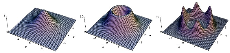
Figure 1: Plots of $\mathcal{E}$ for stationary lump solutions of the $su(2)$ pdCM equation, according to example 1 of section 5.1.1. Here we chose $p=\mathrm{i}$ and $f(\omega)=\omega/2$ (left), $f(\omega)=\omega^{2}/2$ (middle) and $f(\omega)=(\omega^{6}-1)/8$ (right).

Example 2. Let $N=4$ and

$$V=\left(\begin{array}[]{c}\mathcal{I}_{2}\\ \mathcal{I}_{2}\end{array}\right)\;.$$ (5.161)

Then $\varphi$ has the following components,

$$\varphi_{11}=-\varphi_{22}=\frac{1}{\mathcal{D}}\Big{(}\beta_{1}\beta_{2}(ah_{1}^{\ast}h_{2}-a^{\ast}h_{1}h_{2}^{\ast})-\mathrm{i}\,[(\beta_{1}+\beta_{2})|b|^{4}+\beta_{1}|ah_{2}|^{2}+\beta_{2}|ah_{1}|^{2}]\Big{)}\,,$$

$$\varphi_{12}=-\varphi_{21}^{\ast}=\frac{1}{\mathcal{D}}\Big{(}(b^{\ast})^{2}(a\beta_{1}h_{1}+a^{\ast}\beta_{2}h_{2})+a|h_{1}|^{2}\beta_{2}h_{2}+a^{\ast}\beta_{1}h_{1}|h_{2}|^{2}\Big{)}\,,$$ (5.162)

where

$$\beta_{i}=2\,\Im(p_{i})\,,\quad a=p_{1}-p_{2}^{\ast}\,,\quad b=p_{1}-p_{2}\,,$$ (5.163)

$$h_{1}=a\beta_{1}f_{1}\,,\qquad h_{2}=a^{\ast}\beta_{2}f_{2}\,,$$ (5.164)

$$\mathcal{D}=(|b|^{2}+|h_{1}|^{2})(|b|^{2}+|h_{2}|^{2})+\beta_{1}\beta_{2}|h_{1}-h_{2}|^{2}\;.$$ (5.165)

This solution is regular since $\mathcal{D}$ is positive (note that $|b|>0$ since $p_{1}\neq p_{2}$, $|b|^{2}\geq-\beta_{1}\beta_{2}$, and use $|h_{1}|^{2}+|h_{2}|^{2}\geq|h_{1}-h_{2}|^{2}$). Figure 2 shows an example. For generic parameter values, plots of $\mathcal{E}$ show lumps with apparently trivial interaction. But if $p_{1},p_{2}$ are close to the values $\pm\mathrm{i}$ (that correspond to the stationary single lump solutions), a non-trivial interaction is observed in a compact space region, see figure 3. The scalar KP-I equation possesses solutions with the same behaviour [LTG04]. Moreover, also dipolar vortices (modons) of a barotropic equation [McWi+Zabu82] and BPS monopoles [Gibb+Mant86] show such a behaviour in head-on collisions. $\square$

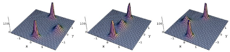
Figure 2: Plots of $\mathcal{E}$ at $t=-2,0,2$ for a three lump solution of the $su(2)$ pdCM equation, according to example 2 of section 5.1.1. Here we chose $p_{1}=\mathrm{i},p_{2}=2\mathrm{i}$, and $f_{1}(\omega_{1})=\omega_{1}^{2}+2$, $f_{2}(\omega_{2})=\omega_{2}/4$. Due to the special choice of $p_{1}$, a pair of lumps is stationary. The positions of the latter are given by the zeros of $f_{1}(\omega_{1})=x^{2}-y^{2}+2-2\mathrm{i}xy$, which are located at $(x,y)=(0,\pm\sqrt{2})$. The position of the third lump corresponds to the zero of $f_{2}(\omega_{2})$, which is given by $(x,y)=(-3t/5,0)$. Choosing $-2$ instead of $+2$ in $f_{1}(\omega_{1})$, all three lumps are located on the line $y=0$, and the third lump moves through both members of the pair (which then reside at $x=\pm\sqrt{2}$).

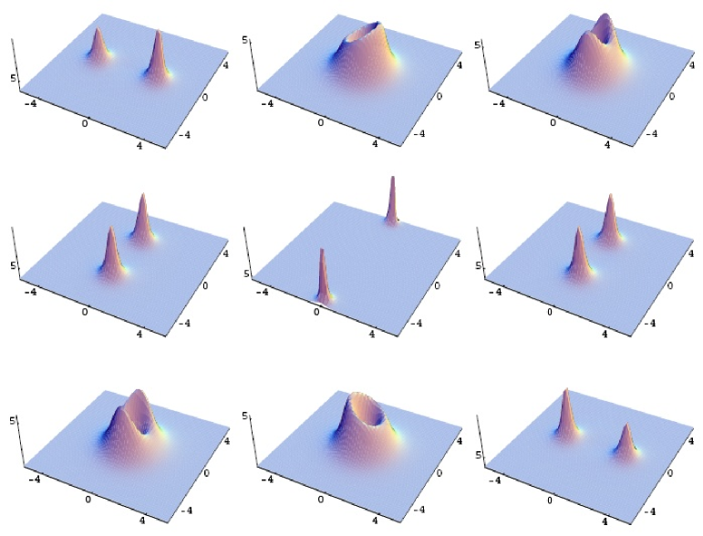
Figure 3: Plots of $\mathcal{E}$ at $t=-110,-100,-99,-90,0,90,99,100,110$ for the solution in example 2 of section 5.1.1 with the data $p_{1}=-19\,\mathrm{i}/20$, $p_{2}=21\,\mathrm{i}/20$, $f_{1}=2\,\mathrm{i}\,\omega_{1}$, $f_{2}=2\,\mathrm{i}\,\omega_{2}$. Two lumps approach each other in $x$-direction, merge, move away from one another in $y$-direction up to some maximal distance, return to each other and merge again, and then separate in $x$-direction.

5.2 Another class of solutions of the $su(m)$ pdCM hierarchy

Let $N$ be even. We introduce the commuting matrices

$$\mathcal{X}_{I}=\left(\begin{array}[]{cc}f_{I}&\tilde{h}_{I}\\ 0&f_{I}\end{array}\right)\,,\quad P_{I}=\left(\begin{array}[]{cc}p_{I}&1\\ 0&p_{I}\end{array}\right)\,,$$ (5.170)

with pairwise different complex constants $p_{I}$, and functions $f_{I},h_{I}$, $I=1,\ldots,N/2$, and construct in terms of them the block-diagonal matrices

$$\mathcal{X}^{\prime}=\left(\begin{array}[]{cccc}\mathcal{X}_{1}&&&\\ &\mathcal{X}_{2}&&\\ &&\ddots&\\ &&&\mathcal{X}_{N/2}\end{array}\right)\,,\quad P=\left(\begin{array}[]{cccc}P_{1}&&&\\ &P_{2}&&\\ &&\ddots&\\ &&&P_{N/2}\end{array}\right)\,,$$ (5.179)

which then obviously also commute. Now (5.106) becomes

$$f_{I,x_{n}}=p_{I}^{n-1}f_{I,x_{1}}\,,\;\tilde{h}_{I,x_{n}}=p_{I}^{n-1}\tilde{h}_{I,x_{1}}+(n-1)p^{n-2}f_{I,x_{1}}\,,$$ (5.180)

where $I=1,\ldots,N/2$ and $n=1,2,\ldots$. Writing

$$\tilde{h}_{I}=h_{I}+\frac{\partial f}{\partial p_{I}}\,,$$ (5.181)

the second equation is turned into $h_{I,x_{n}}=p_{I}^{n-1}h_{I,x_{1}}$, by use of the first. Hence (5.106) is satisfied if, for $I=1,\ldots,N/2$, $f_{I}$ and $h_{I}$ are holomorphic functions of

$$\omega_{I}=\sum_{n\geq 1}x_{n}\,p_{I}^{n-1}$$ (5.182)

(which is (5.141)), and in particular only depend on the variables $x_{1},x_{2},\ldots$ through this combination. In order to explore the consequences of (5.109), we write $K$ and $Q$ as $N/2\times N/2$ matrices, where the components $K_{IJ}$, respectively $Q_{IJ}$, are $2\times 2$ matrices.

Proposition 5

With the matrix $P$ defined in (5.179), and any $Q$, the solution of (5.109) is given by

$$K_{IJ}=\frac{Q_{IJ}}{p_{I}-p_{J}}-\frac{[\Pi_{2},Q_{IJ}]}{(p_{I}-p_{J})^{2}}+\frac{[\Pi_{2},[\Pi_{2},Q_{IJ}]]}{(p_{I}-p_{J})^{3}}$$ (5.183)

for $I\neq J$, and

$$[\Pi_{2},K_{JJ}]=Q_{JJ}\qquad\quad J=1,\ldots,N/2\,,$$ (5.184)

where

$$\Pi_{2}=\left(\begin{array}[]{cc}0&1\\ 0&0\end{array}\right)\;.$$ (5.187)

Proof: We write $P_{I}=p_{I}\,\mathcal{I}_{2}+\Pi_{2}$. Then (5.109), restricted to components with $I\neq J$, takes the form

$$\Big{(}\mathrm{id}+\frac{1}{p_{I}-p_{J}}\,\mathrm{ad}_{\Pi_{2}}\Big{)}K_{IJ}=\frac{Q_{IJ}}{p_{I}-p_{J}}\,,$$

where $\mathrm{ad}_{\Pi}K=[\Pi,K]$. Now (5.183) follows from

$$\Big{(}\mathrm{id}+\frac{1}{p_{I}-p_{J}}\,\mathrm{ad}_{\Pi_{2}}\Big{)}^{-1}=\sum_{k=0}^{2}(-1)^{k}(p_{I}-p_{J})^{-k}\,\mathrm{ad}_{\Pi_{2}}^{k}\,,$$

since $\mathrm{ad}_{\Pi_{2}}^{3}=0$. The diagonal components of (5.109) are $\mathrm{ad}_{\Pi_{2}}K_{JJ}=Q_{JJ}$, which is (5.184). $\square$

Remark. In view of (5.108), we may always assume that the two upper entries of $K_{JJ}$ vanish (since non-vanishing entries can be absorbed into $\mathcal{X}^{\prime}$). Using the matrix $T$ given below in (5.195), the condition (5.136) then implies $K_{2J-1,2J-1}^{\dagger}=\tau_{2}K_{2J,2J}\tau_{2}$, $J=1,\ldots,N/2$, and this requires that $K_{JJ}$ can only have a non-zero entry in the lower left corner. As a consequence of (5.184), $Q_{JJ}$ is then diagonal and has vanishing trace. $\square$

A simple way of satisfying (5.184) is to choose $V$ such that the diagonal blocks $Q_{JJ}$ vanish, and then set $K_{JJ}=0$, $J=1,\ldots,N/2$. This will be done in section 5.2.1.

It remains to satisfy the further anti-Hermiticity conditions.

5.2.1 $su(2)$ lumps with “anomalous” scattering

Let $N$ now be a multiple of $4$. In analogy with (5.149) we set

$$T=\left(\begin{array}[]{ccccc}0&-\tau_{2}&&&\\ \tau_{2}&0&&&\\ &&\ddots&&\\ &&&0&-\tau_{2}\\ &&&\tau_{2}&0\end{array}\right)\quad\mbox{where}\quad\tau_{2}=\left(\begin{array}[]{cc}0&1\\ 1&0\end{array}\right)\,.$$ (5.195)

Then (5.137) means $P_{1}^{\dagger}=\tau_{2}P_{2}\tau_{2},\ldots,P_{N/2-1}^{\dagger}=\tau_{2}P_{N/2}\tau_{2}$, which by use of (5.170) amounts to

$$p_{2J}=p_{2J-1}^{\ast}\qquad\quad J=1,\ldots,N/2\;.$$ (5.196)

Since we address the case $m=2$, $V$ has to be chosen as an $N\times 2$ matrix, which we subdivide into $2\times 2$ blocks $V_{I}$, $I=1,\ldots,N/2$. It follows that

$$Q_{JJ}=\left\{\begin{array}[]{r}-V_{J}V_{J+1}^{\dagger}\,\tau_{2}\\ V_{J}V_{J-1}^{\dagger}\,\tau_{2}\end{array}\quad\mbox{if $J$ is}\quad\right.\begin{array}[]{l}\mbox{odd}\\ \mbox{even}\end{array}\;.$$ (5.201)

Thus, in order to achieve that $Q_{JJ}=0$, we must arrange that

$$V_{2J-1}V_{2J}^{\dagger}=0\qquad\quad J=1,\ldots,N/2\;.$$ (5.202)

Then $Q$ has the following structure

$$Q=\left(\begin{array}[]{ccccc}0&V_{1}V_{1}^{\dagger}&-V_{1}V_{4}^{\dagger}&V_{1}V_{3}^{\dagger}&\cdots\\ -V_{2}V_{2}^{\dagger}&0&-V_{2}V_{4}^{\dagger}&V_{2}V_{3}^{\dagger}&\cdots\\ -V_{3}V_{2}^{\dagger}&V_{3}V_{1}^{\dagger}&0&V_{3}V_{3}^{\dagger}&\cdots\\ -V_{4}V_{2}^{\dagger}&V_{4}V_{1}^{\dagger}&-V_{4}V_{4}^{\dagger}&0&\\ \vdots&\vdots&\vdots&&\ddots\end{array}\right)\,\tau_{2}\;.$$ (5.208)

Example. The simplest case is $N=4$. Excluding degenerate cases, the two blocks $V_{1},V_{2}$ of $V$ should both have rank $1$. Hence $V_{1}=v_{1}u_{1}^{\dagger},V_{2}=v_{2}u_{2}^{\dagger}$ with vectors $u_{J},v_{J}$, $J=1,2$, satisfying $u_{1}^{\dagger}u_{2}=0$. With a unitary transformation $\sigma$ we can achieve that the lower component of $u_{1}$ vanishes. It follows that the upper component of $u_{2}$ also vanishes. By a redefinition of $v_{1},v_{2}$, we obtain $u_{1}^{\dagger}=(1,0)$ and $u_{2}^{\dagger}=(0,1)$, and thus

$$Q_{12}=v_{1}(\tau_{2}v_{1})^{\dagger}=\left(\begin{array}[]{cc}v_{11}v_{12}^{\ast}&|v_{11}|^{2}\\ |v_{12}|^{2}&v_{12}v_{11}^{\ast}\end{array}\right)\,,$$ (5.211)

$$Q_{21}=-v_{2}(\tau_{2}v_{2})^{\dagger}=-\left(\begin{array}[]{cc}v_{21}v_{22}^{\ast}&|v_{21}|^{2}\\ |v_{22}|^{2}&v_{22}v_{21}^{\ast}\end{array}\right)\,,$$ (5.214)

with an obvious notation for the components of $v_{1}$ and $v_{2}$. We should exclude the case when the expression (5.183) for $K$ reduces to the first term on the right hand side, since this leads back to the solution of example 1 in section 5.1. This case is ruled out if $v_{12}$ or $v_{22}$ is different from zero, which suggests to choose $v_{J}=(0,1)$, $J=1,2$, and thus

$$V_{1}=\left(\begin{array}[]{cc}0&0\\ 1&0\end{array}\right)\,,\qquad V_{2}=\left(\begin{array}[]{cc}0&0\\ 0&1\end{array}\right)\;.$$ (5.219)

Then proposition 5 yields

$$K=\left(\begin{array}[]{cc}0&K_{12}\\ -K_{21}&0\end{array}\right)\,,$$ (5.222)

where

$$K_{IJ}=\left(\begin{array}[]{ccc}-(p_{I}-p_{J})^{-2}&-2\,(p_{I}-p_{J})^{-3}\\ (p_{I}-p_{J})^{-1}&(p_{I}-p_{J})^{-2}\end{array}\right)$$ (5.225)

for $I\neq J$. This in turn allows to compute $\Phi$ and then also $\varphi$. The anti-Hermiticity conditions are then satisfied by setting

$$p_{2}=p_{1}^{\ast}\,,\quad f_{2}(\omega_{2})=f_{1}(\omega_{1})^{\ast}\,,\quad h_{2}(\omega_{2})=h_{1}(\omega_{1})^{\ast}\,,$$ (5.226)

and we have $\omega:=\omega_{1}=\omega_{2}^{\ast}$. The result is

$$\varphi_{11}=-\varphi_{22}=-\frac{\mathrm{i}}{\beta^{7}\mathcal{D}}\left(2+\beta^{4}|f|^{2}+\beta^{4}|f+\mathrm{i}\,\beta\tilde{h}|^{2}\right)\,,$$ (5.227)

$$\varphi_{12}=-\varphi_{21}^{\ast}=\frac{1}{\beta^{5}\mathcal{D}}\left(4\,\mathrm{i}\,f-\beta\tilde{h}-\beta^{5}f^{2}\tilde{h}^{\ast}\right)\,,$$ (5.228)

with $\beta=2\Im(p_{1})$, $f=f_{1}(\omega)$, $\tilde{h}=\tilde{h}_{1}$ given by (5.181) in terms of $f$ and $h=h_{1}(\omega)$, and

$$\mathcal{D}=\beta^{-8}(1+\beta^{4}|f|^{2})^{2}+\beta^{-4}|2f+\mathrm{i}\,\beta\tilde{h}|^{2}\;.$$ (5.229)

The solution $\varphi$ is thus regular for any choice of $p_{1}$, with non-vanishing imaginary part, and the holomorphic functions $f,h$. An example with $h=0$ is shown in figure 4. More interesting structures appear for non-constant $h$. Indeed, figure 5 shows two lumps that scatter at an angle of $90^{\circ}$. Choosing $f$ linear in $\omega$ and $h$ proportional to $\omega^{n}$, we observe a $\pi/n$ scattering. Figures 6 and 7 show examples of $60^{\circ}$, respectively $45^{\circ}$ scattering. $\square$

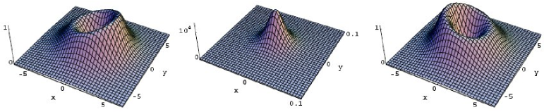
Figure 4: Plots of $\mathcal{E}$ at $t=-50,0,50$ for the solution of section 5.2.1 with the data $p_{1}=\mathrm{i}$ (i.e. $\beta=2$), $f=2\,\omega$ and $h=0$.

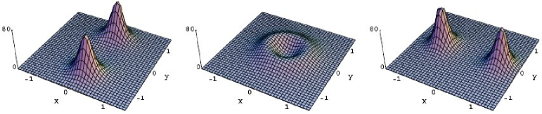
Figure 5: Plots of $\mathcal{E}$ at $t=-5,0,5$ for a 2-lump solution, exhibiting “scattering at right angle”, see section 5.2.1. Here we chose $p_{1}=\mathrm{i}$ and $f=-\mathrm{i}\,\omega/32$, $h=-\omega^{2}/4$.

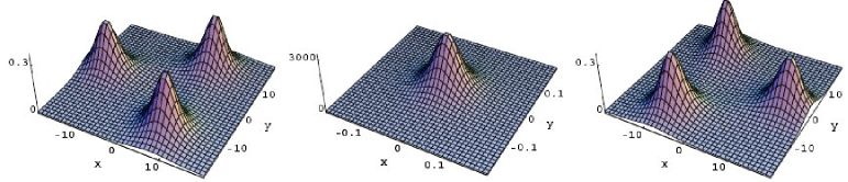
Figure 6: Plots of $\mathcal{E}$ at $t=-500,0,500$ for a 3-lump configuration exhibiting $60^{\circ}$ scattering. This is obtained from the solution of the example in section 5.2.1 with the data $p_{1}=\mathrm{i}$ and $f=-\mathrm{i}\,\omega$, $h=\omega^{3}/8$.

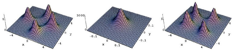
Figure 7: Plots of $\mathcal{E}$ at $t=-20,0,20$ for a 4-lump configuration exhibiting $45^{\circ}$ scattering. This is obtained from the solution of the example in section 5.2.1 with the data $p_{1}=\mathrm{i}$ and $f=-\mathrm{i}\,\omega$, $h=\omega^{4}/8$.

Solutions with $\pi/n$ scattering have also been found in Ward’s chiral model numerically [Sutc92, PSZ92], and analytically as certain limits of families of non-interacting lumps [Ward95, Ioan96, Ioan+Zakr98JMP, Dai+Tern07]. Moreover, also the scalar KP equation (with positive dispersion, i.e. KP I) possesses solutions with this behaviour [GPS93JETP, Peli94, ISS95, Ablo+Vill97, Vill+Ablo99, ACTV00]. In fact, $\pi/n$ scattering in head-on collisions of soliton-like objects is a familiar feature of many models (see [Rose+Sriv91, KPZ93, MacK95], in particular). It occurs in dipolar vortex collisions [McWi+Zabu82, Nguy+Somm88, vanH+Flor89, Voro+Afan92], in $O(3)$ and $\mathbb{C}\mathbb{P}^{1}$ models [Ward85, Lees90, Lees91, Zakr91, PSZ92, Cova+Zakr97, Spei98, Mant+Sutc04], in Skyrme models [Mant87, LPZ90, Sutc91, KPZ93, Mant+Sutc04], for vortices of the Abelian Higgs (or Ginzburg-Landau) model [MMR88, Ruba88, Shel+Ruba88, MRS92, Stra92JMP, Samo92, Mant91, Burz+McCa91, Abde+Burz94, Arth+Burz96, Mant+Sutc04], and BPS monopoles of a $SU(m)$ Yang-Mills-Higgs system [Atiy+Hitc85, AHST85, Gibb+Mant86, Danc+Lees93, Mant+Sutc04]. Another integrable system that possesses solutions with this behaviour is the Davey-Stewartson II equation [Mana+Sant97, Vill+Ablo03] (which can actually be obtained by a multiscale expansion from the KP equation [Zakh+Kuzn86, AMS90]).

The fact that lumps can interact either trivially or non-trivially (in Ward’s chiral model) has been attributed to the status of the internal degrees of freedom in the solutions [Ward95]. But such an explanation appears not to be applicable to the case of the scalar KP equation. This requires further clarification.

5.3 A further generalization

In case of the solutions obtained in section 5.2, the matrix $P$ consists of complex conjugate pairs of $2\times 2$ blocks of Jordan normal form. Of course, this can be generalized to $N_{I}\times N_{I}$ Jordan blocks

$$P_{I}=\left(\begin{array}[]{ccccc}p_{I}&1&0&\cdots&0\\ 0&p_{I}&1&\ddots&\vdots\\ \vdots&\ddots&\ddots&\ddots&\vdots\\ \vdots&&\ddots&p_{I}&1\\ 0&\cdots&\cdots&0&p_{I}\end{array}\right)\,,$$ (5.235)

and $P$ can be chosen as a block-diagonal matrix with pairs of conjugate blocks of this form. For each pair $(P_{I},P_{I}^{\ast})$ in $P$, the matrix $T$ should then have a corresponding block

$$T_{I}=\left(\begin{array}[]{cccccc}&&&&&-1\\ &&&&\iddots&\\ &&&-1&&\\ &&1&&&\\ &\iddots&&&&\\ 1&&&&&\end{array}\right)$$ (5.242)

of size $2N_{I}\times 2N_{I}$, in order to achieve that (5.137) holds.

Example. Let

$$P=\left(\begin{array}[]{cccccc}p&1&&&&\\ 0&p&1&&&\\ &&p&&&\\ &&&p^{\ast}&1&\\ &&&&p^{\ast}&1\\ &&&&0&p^{\ast}\end{array}\right),\;T=\left(\begin{array}[]{cccccc}&&&&&-1\\ &&&&-1&\\ &&&-1&&\\ &&1&&&\\ &1&&&&\\ 1&&&&&\end{array}\right),\;V=\left(\begin{array}[]{cc}0&0\\ 0&0\\ 1&0\\ 0&0\\ 0&0\\ 0&1\end{array}\right)$$ (5.261)

Then $\mathcal{X}^{\prime}$ must have the form

$$\mathcal{X}^{\prime}=\left(\begin{array}[]{cccccc}f&\tilde{h}&\tilde{g}&&&\\ 0&f&\tilde{h}&&&\\ &&f&&&\\ &&&f^{\ast}&\tilde{h}^{\ast}&\tilde{g}^{\ast}\\ &&&&f^{\ast}&\tilde{h}^{\ast}\\ &&&&&f^{\ast}\end{array}\right)\,,$$ (5.269)

and (5.81) becomes

$$f_{x_{n}}=p^{n-1}f_{x_{1}}\,,\qquad\tilde{h}_{x_{n}}=p^{n-1}\tilde{h}_{x_{1}}+(n-1)p^{n-2}f_{x_{1}}\,,$$ (5.270)

$$\tilde{g}_{x_{n}}=p^{n-1}\tilde{g}_{x_{1}}+(n-1)p^{n-1}\tilde{h}_{x_{1}}+\frac{1}{2}(n-1)(n-2)p^{n-3}f_{x_{1}}\;.$$ (5.271)

Writing

$$\tilde{h}=h+\frac{\partial f}{\partial p}\,,\qquad\tilde{g}=g+\frac{\partial h}{\partial p}+\frac{1}{2}\frac{\partial^{2}f}{\partial p^{2}}\,,$$ (5.272)

with functions $f,g,h$, it follows that these equations are satisfied if the latter are arbitrary holomorphic functions of $\omega=\sum_{n\geq 1}p^{n}x_{n}$. Furthermore, we find that

$$K=\left(\begin{array}[]{cc}0&K_{12}\\ -K_{12}^{\ast}&0\end{array}\right)\quad\mbox{with}\quad K_{12}=\left(\begin{array}[]{ccc}\mathrm{i}/\beta^{3}&3/\beta^{4}&-6\mathrm{i}/\beta^{5}\\ 1/\beta^{2}&-2\mathrm{i}/\beta^{3}&-3/\beta^{4}\\ -\mathrm{i}/\beta&-1/\beta^{2}&\mathrm{i}/\beta^{3}\end{array}\right)$$ (5.278)

and $\beta=2\Im(p)$, solves $[P,K]=Q$ with $Q=-VV^{\dagger}T$. The resulting class of solutions is regular since

$$\det(\mathcal{X}^{\prime}-K) = \beta^{-18}(1+\beta^{6}|f|^{2})^{3}+2\beta^{-12}(1+\beta^{6}|f|^{2})|3\mathrm{i}\,f-\beta\tilde{h}|^{2}$$ (5.279)

$$+\beta^{-6}|2f^{2}+(f+\mathrm{i}\,\beta\tilde{h})^{2}+\beta^{2}f\tilde{g}|^{2}+\beta^{-12}|6f+\beta(4\mathrm{i}\,\tilde{h}-\beta\tilde{g})|^{2}\;.$$

Now we have three arbitrary holomorphic functions at our disposal, so this class exhibits quite a variety of different structures. Figures 8 and 9 show some examples. If $h=g=0$, the typical behaviour is similar to the one shown in figure 4. $\square$

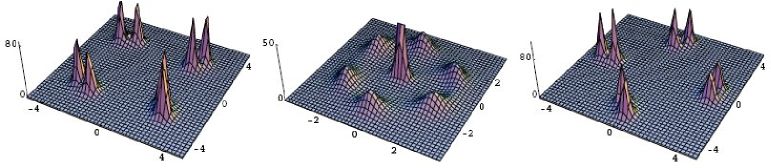
Figure 8: Plots of $\mathcal{E}$ at $t=-20,0,20$ for the solution of the example in section 5.3 with the data $p=\mathrm{i}$, $f=-\mathrm{i}\,\omega$, $h=\omega^{4}/8$ and $g=0$. At $t=0$ we have cut off an extremely large lump in the center.

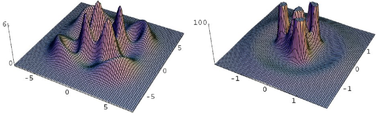
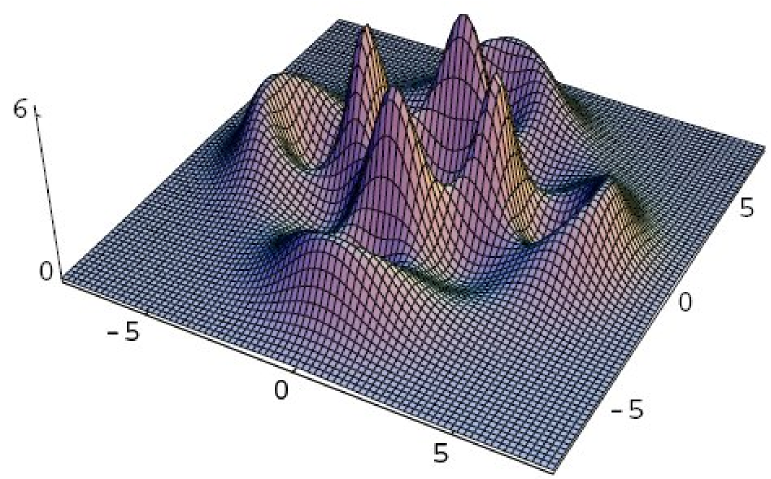
Figure 9: Plots of $\mathcal{E}$ at $t=-1000,0,1000$ for the solution of the example in section 5.3 with the data $p=\mathrm{i}$, $f=-\mathrm{i}\,\omega/40$, $h=\omega^{4}/10$ and $g=0$. At $t=0$ we have cut off the lumps beyond a certain height.

Comparing the data that determine the class of solutions in the example in section 5.2.1, based on a conjugate pair of $2\times 2$ Jordan normal form matrices $P_{I}$, with those of the last example, which is based on a conjugate pair of $3\times 3$ Jordan normal form matrices, there is an obvious generalization to the case of conjugate pairs of larger Jordan normal form matrices $P_{I}$. We note in particular that proposition 5 can be generalized. Since the solutions turned out to be automatically regular in the $2\times 2$ and $3\times 3$ case, it may well be that this holds in general. But a proof of this conjecture is out of reach so far.

5.4 Superposing solutions

The data that determine solutions of the $su(m)$ pdCM hierarchy on the basis of proposition 4 are given by a set of matrices $(P,\mathcal{X}^{\prime},T,V)$. Let two such sets be given, $(P_{i},\mathcal{X}_{i}^{\prime},T_{i},V_{i})$, $i=1,2$, with associated matrices $Q_{i}=-V_{i}V_{i}^{\dagger}T_{i}$, $K_{i}$ (as solutions of (5.109)), and $\Phi_{i}$ given by (5.108). $P_{i},\mathcal{X}_{i},T_{i}$ are $N_{i}\times N_{i}$ matrices and $V_{i}$ is an $N_{i}\times m$ matrix. We can combine them into the larger matrices

$$P=\left(\begin{array}[]{cc}P_{1}&0\\ 0&P_{2}\end{array}\right)\,,\qquad\mathcal{X}^{\prime}=\left(\begin{array}[]{cc}\mathcal{X}^{\prime}_{1}&0\\ 0&\mathcal{X}^{\prime}_{2}\end{array}\right)\,,$$ (5.284)

$$T=\left(\begin{array}[]{cc}T_{1}&0\\ 0&T_{2}\end{array}\right)\,,\qquad\;V=\left(\begin{array}[]{c}V_{1}\\ V_{2}\end{array}\right)\;.$$ (5.289)

Obviously, $(P,\mathcal{X}^{\prime},T,V)$ again satisfies (5.106), (5.107), (5.135), (5.137) and $T^{\dagger}=-T$. (5.133) becomes

$$Q=\left(\begin{array}[]{cc}Q_{1}&Q_{12}\\ Q_{21}&Q_{2}\end{array}\right)\,,\quad Q_{12}=-V_{1}V_{2}^{\dagger}T_{2}\,,\quad Q_{21}=-V_{2}V_{1}^{\dagger}T_{1}\,,$$ (5.292)

and (5.109) with

$$K=\left(\begin{array}[]{cc}K_{1}&K_{12}\\ K_{21}&K_{2}\end{array}\right)$$ (5.295)

yields the equations

$$P_{1}K_{12}-K_{12}P_{2}=Q_{12}\,,\qquad P_{2}K_{21}-K_{21}P_{1}=Q_{21}\;.$$ (5.296)

The off-diagonal blocks of $K$ are a source of complexity and non-triviality of the resulting superposition. (5.136) then determines $K_{21}$ in terms of $K_{12}$ (or vice versa),

$$K_{21}=T_{2}^{-1}K_{12}^{\dagger}T_{1}\;.$$ (5.297)

As a consequence, the second of equations (5.296) follows from the first. If we find a solution $K_{12}$ of the remaining equation, then we obtain

$$\Phi=\left(\begin{array}[]{cc}\Phi_{1}&\Phi_{1}K_{12}\Phi_{2}\\ \Phi_{2}K_{21}\Phi_{1}&\Phi_{2}\end{array}\right)\left(\begin{array}[]{cc}A_{1}^{-1}&0\\ 0&A_{2}^{-1}\end{array}\right)\,,$$ (5.302)

where

$$A_{1}=\mathcal{I}_{N_{1}}-K_{12}\Phi_{2}K_{21}\Phi_{1}\,,\qquad A_{2}=\mathcal{I}_{N_{2}}-K_{21}\Phi_{1}K_{12}\Phi_{2}\,,$$ (5.303)

and $\varphi$ given by (5.132) solves the $su(m)$ pdCM hierarchy, provided that the inverses of $A_{1}$ and $A_{2}$ exist. If the two matrices $\Phi_{i}$ are regular (and thus also the corresponding solutions $\varphi_{i}$), then $\Phi$ and thus also $\varphi$ is regular if and only if $\det(A_{1})\det(A_{2})\neq 0$ (for all values of $x_{1},x_{2},\ldots$). Since $\det(A_{1})=\det(A_{2})$ by an application of Sylvester’s determinant theorem, this reduces to the condition

$$\det(A_{1})\neq 0\;.$$ (5.304)

We note also that $\det(A_{1})$ is real since

$$\det(A_{1})^{\ast} = \det(A_{1}^{\dagger})=\det(\mathcal{I}_{N_{1}}-K_{21}^{\dagger}\Phi_{2}^{\dagger}K_{12}^{\dagger}\Phi_{1}^{\dagger})$$ (5.305)

$$= \det(\mathcal{I}_{N_{1}}-T_{1}K_{12}\Phi_{2}K_{21}\Phi_{1}T_{1}^{-1})=\det(A_{1})\;.$$

Example. We choose

$$P_{1} = \left(\begin{array}[]{cccc}p_{1}&1&&\\ 0&p_{1}&&\\ &&p_{1}^{\ast}&1\\ &&0&p_{1}^{\ast}\\ \end{array}\right)\,,\;\mathcal{X}^{\prime}_{1}=\left(\begin{array}[]{cccc}f_{1}&h_{1}+\partial f_{1}/\partial p_{1}&&\\ 0&f_{1}&&\\ &&f_{1}^{\ast}&h_{1}^{\ast}+(\partial f_{1}/\partial p_{1})^{\ast}\\ &&0&f_{1}^{\ast}\\ \end{array}\right)\,,$$ (5.314)

$$T_{1} = \left(\begin{array}[]{cccc}&&&-1\\ &&-1&\\ &1&&\\ 1&&&\\ \end{array}\right)\,,\;V_{1}=\left(\begin{array}[]{cc}0&0\\ 1&0\\ 0&0\\ 0&1\\ \end{array}\right)\,,$$ (5.323)

where $f_{1},h_{1}$ are arbitrary holomorphic functions of $\omega_{1}$ (with $\omega_{1}$ defined in (5.141)), and

$$P_{2}=\left(\begin{array}[]{cc}p_{2}&0\\ 0&p_{2}^{\ast}\end{array}\right)\,,\;\mathcal{X}^{\prime}_{2}=\left(\begin{array}[]{cc}f_{2}&0\\ 0&f_{2}^{\ast}\end{array}\right)\,,\;T_{2}=\left(\begin{array}[]{cc}0&-1\\ 1&0\end{array}\right)\,,\;V_{2}=\left(\begin{array}[]{cc}1&0\\ 0&1\end{array}\right)\,,\quad$$ (5.332)

with an arbitrary holomorphic function $f_{2}$ of $\omega_{2}$. Thus we superpose data corresponding to a regular solution of the kind treated in the example in section 5.2.1 and data corresponding to a regular solution as given in example 1 of section 5.1. In the following we assume that

$$p_{1}\neq p_{2}\,,\qquad p_{1}\neq p_{2}^{\ast}\;.$$ (5.333)

Together with the conditions $p_{i}\neq p_{i}^{\ast}$, $i=1,2$, which the data of the components have to satisfy, this means that the constants $p_{i}$ and their complex conjugates are pairwise different. The second condition in (5.333) is in fact needed for the matrix $K$ to exist. $K$ has the form (5.295), where $K_{1}$ is given by the $4\times 4$ matrix $K$ in (5.222) with the pair $(p_{1},p_{1}^{\ast})$. Furthermore,

$$K_{2}=\left(\begin{array}[]{cc}0&\frac{1}{p_{2}-p_{2}^{\ast}}\\ \frac{1}{p_{2}-p_{2}^{\ast}}&0\end{array}\right),\;K_{21}=\left(\begin{array}[]{cccc}0&0&-\frac{1}{p_{1}^{\ast}-p_{2}}&\frac{1}{(p_{1}^{\ast}-p_{2})^{2}}\\ \frac{1}{p_{1}-p_{2}^{\ast}}&-\frac{1}{(p_{1}-p_{2}^{\ast})^{2}}&0&0\end{array}\right),$$ (5.338)

and $K_{12}$ is then determined by (5.297). With some efforts the expression for $\det(A_{1})$ can be brought into the form

$$\det(A_{1}) = |a|^{-8}(1+\beta_{2}^{2}|f_{2}|^{2})^{-1}\left(|w|^{2}+(1+\beta_{1}^{4}|f_{1}|^{2})^{2}\right)^{-2}\Big{[}\Big{(}|a|^{4}[\,|w|^{2}+(1+\beta_{1}^{4}|f_{1}|^{2})^{2}\,]$$ (5.339)

$$-\beta_{1}\beta_{2}\,[\,|a|^{2}(1+\beta_{1}^{4}|f_{1}|^{2})+|b|^{2}+|aw+\mathrm{i}b^{\ast}\beta_{1}^{2}f_{1}|^{2}\,]\Big{)}^{2}$$

$$+\Big{|}(a^{\ast})^{4}(|w|^{2}+(1+\beta_{1}^{4}|f_{1}|^{2})^{2})\beta_{2}f_{2}$$

$$+\beta_{1}\beta_{2}\Big{(}b^{2}w+(a^{\ast})^{2}\beta_{1}^{4}f_{1}^{2}w^{\ast}-2\mathrm{i}a^{\ast}b\beta_{1}^{2}f_{1}(1+\beta_{1}^{4}|f_{1}|^{2})\Big{)}\Big{|}^{2}\,\Big{]}\,,$$

where

$$\beta_{i}=2\,\Im(p_{i})\,,\quad a=p_{1}-p_{2}^{\ast}\,,\quad b=p_{1}-p_{2}\,,\quad w=\beta_{1}^{3}h_{1}-2\mathrm{i}\,\beta_{1}^{2}f_{1}\;.$$ (5.340)

The regularity condition (5.304) turns out to be automatically satisfied. This is seen as follows. First we note that

$$|a|^{4}=|b|^{4}+\beta_{1}\beta_{2}\,(|a|^{2}+|b|^{2})>\beta_{1}\beta_{2}\,(|a|^{2}+|b|^{2})\,,$$ (5.341)

as a consequence of the first of the inequalities (5.333), and thus

$$|a|^{4}\,(1+\beta_{1}^{4}|f_{1}|^{2})^{2}>\beta_{1}\beta_{2}\,(|a|^{2}+|b|^{2})(1+\beta_{1}^{4}|f_{1}|^{2})\;.$$ (5.342)

Using $|a|^{2}>\beta_{1}\beta_{2}$, this leads to

$$|a|^{4}\,(|w|^{2}+(1+\beta_{1}^{4}|f_{1}|^{2})^{2}) > \beta_{1}\beta_{2}\,\left(|a|^{2}(1+\beta_{1}^{4}|f_{1}|^{2})+|b|^{2}+|aw|^{2}+|\mathrm{i}\,b^{\ast}\beta_{1}^{2}f_{1}|^{2}\right)$$ (5.343)

$$\geq \beta_{1}\beta_{2}\,\left(|a|^{2}(1+\beta_{1}^{4}|f_{1}|^{2})+|b|^{2}+|aw+\mathrm{i}\,b^{\ast}\beta_{1}^{2}f_{1}|^{2}\right)\,,$$

which implies $\det(A_{1})>0$.

Figure 10 shows plots of $\mathcal{E}$ at consecutive times, for a special choice of the data. $\square$

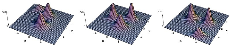
Figure 10: Plots of $\mathcal{E}$ at $t=-2,0,2$ for a superposition of a 2-lump configuration, with “anomalous scattering”, and a single lump (which is at the top of the left plot and at the bottom of the right plot), according to the example of section 5.4. Here we chose $p_{1}=\mathrm{i}$, $p_{2}=-3\mathrm{i}/8$, $f_{1}=-\mathrm{i}\,\omega_{1}/32$, $f_{2}=24\,\omega_{2}$, and $h_{1}=-\omega^{2}/4$.

In the last example the regularity of the superposition turned out to be a consequence of the “regular data” we started with. But this example also demonstrates that it is quite difficult in general to evaluate the regularity condition (5.304). We note that also the cases treated in sections 5.1.1 and 5.2.1 may be regarded as special cases of “superpositions” as formulated above. In particular, example 2 of section 5.1.1 provides us with another example where the superposition of regular data turned out to be regular again. It is unlikely that this is a special feature of our particular examples. But in order to tackle a general proof, we probably need different methods.

6 Conclusions

We summarize the relations between integrable systems and their hierarchies considered in this work in the following diagram.