Gap solitons in spatiotemporal photonic crystals

Abstract

We generalize the concept of nonlinear periodic structures to systems that show arbitrary spacetime variations of the refractive index. Nonlinear pulse propagation through these spatiotemporal photonic crystals can be described, for shallow nonstationary gratings, by coupled mode equations which are a generalization of the traditional equations used for stationary photonic crystals. Novel gap soliton solutions are found by solving a modified massive Thirring model. They represent the missing link between the gap solitons in static photonic crystals and resonance solitons found in dynamic gratings.

The ability to manipulate spectrally and temporally optical pulses has been a longstanding goal in modern science and technology, and periodic media have the potential of engineering light propagation to an unprecedented degree [1]. Systems possessing a periodic modulation of refractive index, in which photonic bandgaps (PBGs) form at or near a multiple of the Bragg frequency (or wavenumber), have been used in a wide range of applications, including dispersion compensators and optical filters [1]. When Kerr nonlinearity is considered, new effects come into play, such as optical bistability, pulse compression, optical switching and soliton formation [1].

Stationary gap solitons (GSs) living in the frequency bandgap of a 1D periodic medium were first investigated in 1987-1989 in a series of fundamental papers [2, 3, 4], and found experimentally in 1996 [5]. Solitons living in a wavenumber bandgap of the so-called dynamic gratings (i.e. a traveling-wave periodic index change) were also investigated in Refs. [9, 11, 10] by using copropagating beams, where the complementarity between the two kinds of bandgap was evident. Since then, there has been an exponential increase in the number of studies and practical applications of GSs. An intriguing possibility is the storage of optical pulses in the form of zero velocity GSs followed by release from the structure at a controllable delay [1].

Much less attention, however, has been devoted to the physics of nonstationary periodic media, such as dielectric structures showing temporal variations of the refractive index [6, 7], which have the potential to dramatically enhance the degree of spectral control over light pulses by periodic media thanks to the new temporal degree of freedom [6]. In Ref. [7] we derived the transfer matrix $\mathcal{T}$ for plane waves scattered by the sharp boundary associated with a medium with time-varying refractive index, which must be distinguished from a moving interface in that the medium itself is immobile [7, 8]. The knowledge of $\mathcal{T}$ for a single boundary allowed us to construct a theory for more complicated nonstationary dielectric objects. In particular in [7] we introduced the important concept of spatiotemporal photonic crystal (STPC), which is a grating that shows a well-defined periodicity of the refractive index along a certain direction of the spacetime plane $(z,ct)$ ($z$ is the longitudinal spatial coordinate, $t$ is time and $c$ is the speed of light). This periodicity gives rise to PBGs in a mixed frequency-wavenumber space, the mixing being regulated by an angular parameter $\theta$, which we shall see it is related to the apparent velocity of the layers in the spacetime plane.

In this Letter we extend the linear theory formulated in Ref. [7] to nonstationary gratings with Kerr nonlinearity, demonstrating the existence of self-localized solutions in the mixed frequency-wavenumber bandgaps of STPCs, thus showing that the conventional concept of GS (see Refs. [2, 3, 4, 9, 10]) must be extended to encompass general spacetime variations of the refractive index.

Let us consider an electromagnetic wave, with its electric and magnetic fields $\mathbf{E}=(E(z,t),0,0)$ and $\mathbf{B}=(0,B(z,t),0)$ linearly polarized along the $\hat{x}$ and $\hat{y}$ directions respectively. $E$ and $B$ depend on $z$ and $t$ only, because we assume conditions of normal incidence, so that any change of the time-dependent refractive index occurs along $\hat{z}$. The linear polarization $\mathbf{P}_{L}$ of the medium is given by $\mathbf{P}_{L}=\chi_{L}(z,t)\mathbf{E}=[n(z,t)^{2}-1]\mathbf{E}$, where $\chi_{L}$ is the linear susceptibility of the (non-magnetic) medium and $n(z,t)$ is the linear refractive index, which is assumed for simplicity to be real and frequency independent, and possessing for the moment an arbitrary dependence on $z$ and $t$. Maxwell’s equations for $E$ and $B$ are $\partial_{t}(\epsilon E)+c\partial_{z}B+\partial_{t}P_{NL}=0$, $\partial_{t}B+c\partial_{z}E=0$, where $\epsilon(z,t)\equiv 1+\chi_{L}=n(z,t)^{2}$, and $P_{NL}$ is the Kerr nonlinear polarization, $P_{NL}=\chi_{NL}E^{3}$, with $\chi_{NL}$ constant. Here and in the following we use the Heaviside-Lorentz units system, see Ref. [8].

By deriving the first of Maxwell’s equations with respect to $t$, and using the second one to eliminate $B$, we obtain the nonlinear wave equation for a space- and time-varying refractive index:

$$\epsilon\partial_{t}^{2}E-c^{2}\partial_{z}^{2}E+(\partial_{t}^{2}\epsilon)E+2(\partial_{t}\epsilon)(\partial_{t}E)+\partial_{t}^{2}P_{NL}=0.$$ (1)

It is now convenient to introduce two new variables, rotated by an angle $\theta\in[-\pi/2,\pi/2]$ in the $(z,ct)$ plane: $p=\cos(\theta)z-\sin(\theta)ct,q=\sin(\theta)z+\cos(\theta)ct$. This spacetime rotation is analogous to the Lorentz transformations in special relativity, with the essential conceptual difference that in our case the associated dimensionless velocity $\beta\equiv\tan(\theta)$ can assume values in the range $0<|\beta|<\infty$, and it is not limited by $c$, see Ref. [7] and references therein. $p$ will be chosen to correspond to the direction parallel to the periodicity of the STPC, while $q$ will be orthogonal to $p$. $\theta>0$ implies that the boundaries of the STPC are moving towards light, while for $\theta<0$ the boundaries are moving away from the incident pulse. A generalized plane wave propagating in the $(p,q)$ space has the form $\Psi=\Psi_{0}\exp(i\tilde{k}p-i\tilde{\omega}q)$, where $\Psi_{0}$ is a constant amplitude, and $\tilde{k}$ and $\tilde{\omega}$ are the wavenumbers associated to the $p$ and $q$ directions respectively. $\tilde{k}$ and $\tilde{\omega}$ are linked by the rotation $\tilde{k}=\cos(\theta)k+\sin(\theta)\omega/c$ and $\tilde{\omega}=\cos(\theta)\omega/c-\sin(\theta)k$, where $k$ and $\omega/c$ are the wavenumbers associated to the original physical plane $(z,ct)$. Figure 1 shows the geometrical meaning of axes $p$ and $q$ for three representative STPCs of fundamental importance (see caption). It is evident from the above definitions that the case $\theta\rightarrow 0$ corresponds to layers arranged periodically along $z$ ($p\rightarrow z$), and the plane wave delocalization direction lies along $ct$ ($q\rightarrow ct$). This corresponds to the traditional time-independent photonic crystal, see Fig. 1(a). Being the crystal invariant with respect to translations along $ct$, we name this structure a space-like STPC. More interesting is the second limiting case, when $\theta\rightarrow\pm\pi/2$, shown in Fig. 1(b). From the definitions of $p$ and $q$, we have $p\rightarrow\mp ct$ and $q\rightarrow\pm z$, so that plane waves will be delocalized along $z$, and all the variations of refractive index occur in time only. In analogy with the previous nomenclature, we name this structure a time-like STPC, an example of which is the dynamic grating [11, 9]. The intermediate cases when $0<|\theta|<\pi/2$, which are the main focus of this Letter, are displayed schematically in Fig. 1(c).

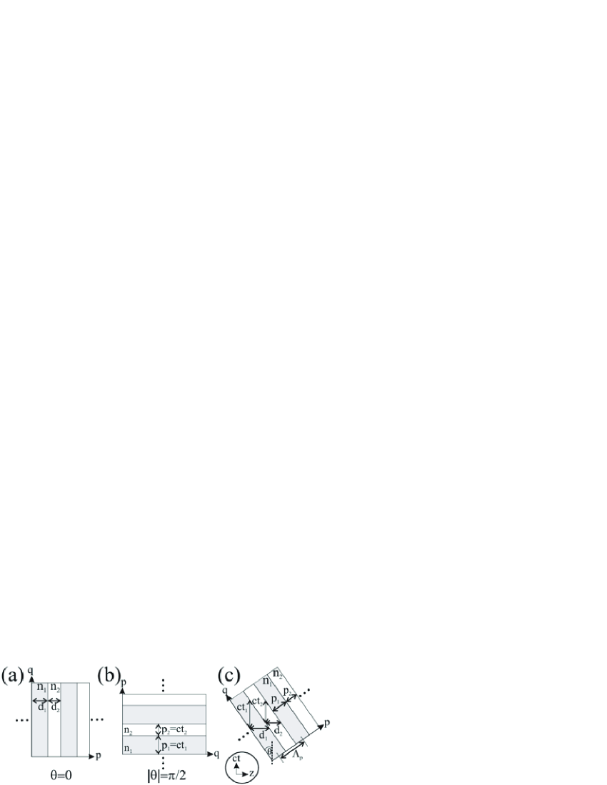
Figure 1: (a) Space-like, conventional static photonic crystal ($\theta=0$), for which $p=z$ and $q=ct$. $n_{1,2}$ and $d_{1,2}$ are respectively refractive indices and widths of the two types of layers. (b) Time-like photonic crystal, $\theta=\pm\pi/2$, for which the refractive index changes periodically in time only ($p=-ct$), and $q=z$. $ct_{1,2}$ are the durations of the layers. (c) Intermediate case $0<|\theta|<\pi/2$. $\Lambda_{p}$ is the period of the structure along the grating direction. Axis $ct$ and $z$ are indicated in a circle.

In principle, integration of Eq.(1) is all one needs to completely solve the problem of nonlinear pulse propagation in any kind of nonstationary dispersionless structure. However, one can gain important analytical insight by considering a cosinusoidal shallow grating described by the dielectric function $\epsilon(p)=n_{0}^{2}+\mu[\exp(i\tilde{k}_{B}p)+\textrm{c.c.}]$, where $n_{0}^{2}$ is the square of the average linear refractive index, and $\mu\ll n_{0}^{2}$. Here, $\tilde{k}_{B}$ represents the equivalent of the Bragg wavenumber along $p$. The Bragg condition, which is the phase-matching condition between the optical and the grating wavenumbers, is given by $\tilde{k}_{B}=\tilde{k}^{+}-\tilde{k}^{-}$. Due to the fact that only two Fourier modes are present in the above expression for $\epsilon(p)$, we can assume that only two optical modes strongly contribute to the propagation dynamics, which leads us to the expansion $E(p,q)=[F(p,q)e^{i\tilde{k}^{+}p-i\tilde{\omega}q}+B(p,q)e^{i\tilde{k}^{-}p-i\tilde{\omega}q}+\textrm{c.c.}]/2$, where $F$ and $B$ are envelopes of respectively the forward and backward components of the electric field, $\tilde{k}^{\pm}$ are the wavenumbers along $p$ for $F$ and $B$ respectively, and $\tilde{\omega}$ is the wavenumber along $q$, which is common for both components. Note that: (i) here the terms ’forward’ and ’backward’ are not in general associated to the spatial motion of the modes (unless $\theta=0$), but rather to the more general motion along the $p$-direction, and (ii) the $F$ and $B$ modes will generally have different linear wavenumbers $|\tilde{k}^{\pm}|$ along $p$. The dispersion relation between $\tilde{k}^{\pm}$ and $\tilde{\omega}$ is (see also [7]) $\tilde{k}^{\pm}=[\sin(\theta)\pm n_{0}\cos(\theta)]\tilde{\omega}/[\cos(\theta)\mp n_{0}\sin(\theta)]$, which is not valid for $\theta=\pm\arctan(1/n_{0})$. For those angles, either $k^{+}$ or $k^{-}$ diverge and the wavenumber along the $p$-direction is not defined. Physically this is due to the fact that for $\theta<-\arctan(1/n_{0})$ the layers boundaries of the STPC are changing faster than the speed of light in the medium ($c/n_{0}$).

After substituting the expansion for $E(p,q)$ into Eq.(1), a slowly-varying amplitude approximation (SVEA) in $p$ and $q$ is performed: $|\partial_{p}^{2}\psi|\ll|\tilde{k}^{\pm}\partial_{p}\psi|\ll|(\tilde{k}^{\pm})^{2}\psi|,|\partial_{q}^{2}\psi|\ll|\tilde{\omega}\partial_{q}\psi|\ll|\tilde{\omega}^{2}\psi|$, where $\psi$ is either $F$ or $B$, and similar relations are valid for the terms containing the mixed derivative $\partial_{p}\partial_{q}$. The following two spatiotemporal coupled mode equations (STCMEs) are obtained:

$$i\partial_{p}F+\frac{n_{0}\cos(\theta)+\sin(\theta)}{\cos(\theta)-n_{0}\sin(\theta)}i\partial_{q}F+\frac{\kappa}{[\cos(\theta)-n_{0}\sin(\theta)]^{2}}B+\frac{\Gamma}{[\cos(\theta)-n_{0}\sin(\theta)]^{2}}(|F|^{2}+2|B|^{2})F=0,$$ (2)

$$-i\partial_{p}B+\frac{n_{0}\cos(\theta)-\sin(\theta)}{\cos(\theta)+n_{0}\sin(\theta)}i\partial_{q}B+\frac{\kappa}{[\cos(\theta)+n_{0}\sin(\theta)]^{2}}F+\frac{\Gamma}{[\cos(\theta)+n_{0}\sin(\theta)]^{2}}(2|F|^{2}+|B|^{2})B=0,$$ (3)

where $\Gamma\equiv(3\tilde{\omega}\chi_{NL})/(8n_{0})$ is the nonlinear coefficient, and $\kappa\equiv\tilde{\omega}\mu/(2n_{0})$ is the grating coupling constant. Again, the equations have a singular character for $\theta=\pm\arctan(1/n_{0})$. Eqs.(2-3) represent the first central result of this Letter. Let us now perform the following scaling, which is well-defined for $\theta\neq\arctan(1/n_{0})$ and $\theta\neq-\arctan(n_{0})$: $\tau=q/q_{0}$, $\xi=p/p_{0}$, $f=F/A_{0}$, $b=B/A_{0}$, with $p_{0}\equiv\kappa^{-1}[\cos(\theta)-n_{0}\sin(\theta)]^{2}$, $q_{0}\equiv[n_{0}\cos(\theta)+\sin(\theta)]p_{0}/[\cos(\theta)-n_{0}\sin(\theta)]$, $F_{0}\equiv(\kappa/\Gamma)^{1/2}$. With this, equations (2-3) are reduced to the following two dimensionless equations:

$$i\left(\partial_{\xi}+\partial_{\tau}\right)f+b+\left(2|b|^{2}+|f|^{2}\right)f=0,$$ (4)

$$i\left(-\partial_{\xi}+\rho_{1}\partial_{\tau}\right)b+\rho_{2}f+\rho_{2}\left(2|f|^{2}+|b|^{2}\right)b=0,$$ (5)

where $\rho_{1}(\theta)\equiv[n_{0}\cos(\theta)-\sin(\theta)][\cos(\theta)-n_{0}\sin(\theta)]/\{[\cos(\theta)+n_{0}\sin(\theta)][n_{0}\cos(\theta)+\sin(\theta)]\}$ and $\rho_{2}(\theta)\equiv\{[\cos(\theta)-n_{0}\sin(\theta)]/[\cos(\theta)+n_{0}\sin(\theta)]\}^{2}$. In Figure 2(a) coefficients $\rho_{1,2}$ are shown as a function of $\theta$ for an average refractive index $n_{0}=3$. Note that although $\rho_{2}$ is always positive in the range $\theta\in[-\pi/2,\pi/2]$, $\rho_{1}$ becomes negative for $\arctan(1/n_{0})<|\theta|<\arctan(n_{0})$, and shows two divergences for negative angles at $\theta=-\arctan(n_{0})$ and at $\theta=-\arctan(1/n_{0})$. Also $\rho_{1}=\rho_{2}=1$ for the limiting cases $\theta=0$ and $\theta=\pi/2$, but in general these parameters can strongly differ from unity.

Let us now discuss the most important linear property of Eqs.(4-5), namely the PBG in the $\theta$-rotated frequency-wavenumber space. Substituting $\{f,b\}=\Psi_{f,b}\exp(ik^{\prime}\xi-i\omega^{\prime}\tau)$ into Eqs.(4-5), and neglecting the nonlinear terms, we readily obtain $\omega^{\prime}_{1,2}(\theta)=\{(\rho_{1}-1)k^{\prime}\pm[(1+\rho_{1})^{2}k^{\prime 2}+4\rho_{1}\rho_{2}]^{1/2}\}/(2\rho_{1})$, after which we perform an inverse rotation back to the original dimensionless frequency-wavenumber space, i.e. $k^{\prime\prime}=\cos(\theta)k^{\prime}-\sin(\theta)\omega^{\prime}$, $\omega^{\prime\prime}=\sin(\theta)k^{\prime}+\cos(\theta)\omega^{\prime}$. In Figure 2(d,e,f) the bandstructure $\omega^{\prime\prime}_{1,2}(k^{\prime\prime})$ for three different cases ($\theta=0$, $\theta=1.3$ and $\theta=\pi/2$) is plotted, explicitly showing the passage from the frequency bandgap [$\theta=0$, Fig. 2(d)] to the wavenumber bandgap [$\theta=\pi/2$, Fig. 2(f)], passing through a region in which the two kinds of bandgap coexist [$\theta=1.3$, Fig. 2(e)].

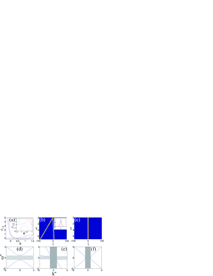
Figure 2: (Color online) (a) $\theta$-dependence of coefficients $\rho_{1,2}$ for the parameter range $\theta\in[-\arctan(1/n_{0}),\pi/2]$, and for $\theta\in[-\pi/2,0]$ (inset). (b) Contour plot of $I_{tot}=|f|^{2}+|b|^{2}$ for numerical propagation of an initial STGP (input profile shown inset, blue line is $|f|$ and red line is $|b|$) with parameters $v=0$, $\theta=1.3$ and $\delta=\pi/2$, without grating ($\kappa=0$). Propagation length is $\tau=7$. (c) Same as (b) but with grating coupling. (d) Bandstructure in space $(k^{\prime\prime},\omega^{\prime\prime})$ as calculated by using (4-5), for $\theta=0$, (e) for $\theta=1.3$ and (f) for $\theta=\pi/2$. In (c,d,e), light gray regions indicate the $\omega^{\prime\prime}$-bandgap, and the dark gray regions the $k^{\prime\prime}$-bandgap. In all cases $n_{0}=3$.

We now proceed to analyze the symmetries and the GS solutions of Eqs.(4-5). One can derive Eqs.(4-5) from the following Hamiltonian density: $\mathcal{H}=(bf^{*}+fb^{*})+2|f|^{2}|b|^{2}+(|f|^{4}+|b|^{4})/2-\mathcal{M}_{f}+\mathcal{M}_{b}/\rho_{2}$, where the star indicates complex conjugation, and where $\mathcal{M}_{\zeta}\equiv i(\zeta\partial_{\xi}\zeta^{*}-\textrm{c.c.})/2=\textrm{Im}\left\{\zeta^{*}\partial_{\xi}\zeta\right\}$ is the momentum density of the generic field $\zeta=\{f,b\}$. The dynamical equations are written as $i\hat{J}\hat{M}\partial_{\tau}\mathbf{g}+\delta\mathcal{H}/\delta\mathbf{g}^{\dagger}=0$, where $\hat{M}\equiv\textrm{diag}(1,\rho_{1}/\rho_{2})$, $\hat{J}\equiv\textrm{diag}(1,-1)$ is the symplectic matrix, $\mathbf{g}\equiv[f,b]$ is the field vector, and dagger indicates hermitian conjugation. Moreover, the variational derivative is given by $\delta/(\delta\zeta)\equiv\partial/(\partial\zeta)-\partial_{\xi}[\partial/\partial(\partial_{\xi}\zeta)]$, see also Ref. [12]. We anticipate that $\xi$ will correspond to the localization coordinate of the soliton solutions, and $\tau$ to the evolution coordinate. With this in mind, one can find the total Hamiltonian by integrating $\mathcal{H}$ over $\xi$, $H=\int_{-\infty}^{+\infty}\mathcal{H}d\xi\equiv[\mathcal{H}]_{-\infty}^{+\infty}$. $H$ is an integral of motion, i.e. $\partial_{\tau}H=0$. $\mathcal{H}$ does not depend on the variable $\xi$ explicitly, leading to the conservation of total momentum: $M_{tot}=[\mathcal{M}_{f}+(\rho_{1}/\rho_{2})\mathcal{M}_{b}]_{-\infty}^{+\infty}$, i.e. $\partial_{\tau}M_{tot}=0$. $\mathcal{H}$ is also invariant with respect to the ’gauge transformation’ $f\rightarrow f\exp(i\phi)$, $b\rightarrow b\exp(i\phi)$, leading to the conservation of the quantity $P=[|f|^{2}+(\rho_{1}/\rho_{2})|b|^{2}]_{-\infty}^{+\infty}$, and $\partial_{\tau}P=0$. The number of integrals of motion of the dynamical system determined by (4-5) (with the exclusion of $H$) is closely related to the number of internal parameters of the corresponding soliton families [13]. Therefore the family of localized solutions living inside the $\tilde{\omega}$-bandgap of a STPC are represented by two internal parameters. This is well-known for solitons living in the frequency bandgap of a static photonic crystal ($\theta=0$) [3, 4], and for GSs living in the wavenumber bandgap ($\theta=\pm\pi/2$) [9, 10], but our analysis extends this result for arbitrary values of $\theta$.

In order to find analytical localized solutions of Eqs.(4-5), let us now consider the following different set of coupled equations for two new fields $\psi_{f}$ and $\psi_{b}$:

$$i\left(\partial_{\xi}+\partial_{\tau}\right)\psi_{f}+\psi_{b}+|\psi_{b}|^{2}\psi_{f}=0,$$ (6)

$$i\left(-\partial_{\xi}+\rho_{1}\partial_{\tau}\right)\psi_{b}+\rho_{2}\psi_{f}+\rho_{2}|\psi_{f}|^{2}\psi_{b}=0.$$ (7)

In analogy with the extensively studied Massive Thirring Model (MTM) [14, 4], we name Eqs.(4-5) the modified Massive Thirring Model (mMTM). The MTM is a particular case of the mMTM, with $\rho_{1}=\rho_{2}=1$, and it is known to be integrable [14]. The mMTM solitons will automatically provide analytical soliton solutions to the original equations Eqs.(4-5). Let us operate the Galileian shift $\tau^{\prime}=\tau-V\xi$, $\xi^{\prime}=\xi$, and the rescalings $\bar{\tau}=\tau^{\prime}/\tau_{0}$ and $\bar{\xi}=\xi^{\prime}$. By choosing $\tau_{0}=1+V$ and $V=(1-\rho_{1})/2$ we can therefore scale $\rho_{1}$ away from Eqs.(6-7). It is now possible to find the following analytical soliton solution:

$$\psi_{f}(\bar{\xi},\bar{\tau})=(1/\Delta)\psi_{0},\qquad\psi_{b}(\bar{\xi},\bar{\tau})=-\Delta\psi_{0},$$ (8)

where $\psi_{0}=\sin(\delta)\textrm{sech}\left(\Theta-i\delta/2\right)\exp(i\sigma)$, $\gamma=\left[\rho_{2}/(1-v^{2})\right]^{1/2}$, $\Delta=[\rho_{2}(1-v)/(1+v)]^{1/4}$, $\Theta=\gamma\sin(\delta)(\bar{\xi}-v\bar{\tau})=\gamma\sin(\delta)\{[1+vV/(1-V)]\xi-V\tau/(1-V)\}$ and $\sigma=\gamma\cos(\delta)(v\bar{\xi}-\bar{\tau})=\gamma\cos(\delta)\{[v+V/(1-V)]\xi-\tau/(1-V)\}$. $0<\delta<\pi$ is a parameter (also called the soliton charge) which measures the detuning from the bandgap center ($\delta=\pi/2$), and $-1\leq v\leq+1$ is the soliton relative velocity.

We now attempt to express the general localized solutions of Eqs.(4-5) in terms of mMTM solitons, Eqs.(8), by using the ansatz: $\{f,b\}=\alpha\psi_{f,b}(\xi,\tau)\exp[i\eta(\Theta(\xi,\tau))]$. Substituting into Eqs.(4-5) and using (8), we obtain two equations for $\eta^{\prime}\equiv\partial_{\Theta}\eta$. The consistency condition between them determines the value of $\alpha$: $\alpha=\{[2(1-v^{2})\rho_{2}]/[(1+v)^{2}+4(1-v^{2})\rho_{2}+(1-v)^{2}\rho_{2}^{2}]\}^{1/2}$, which in turn is used to solve the ODE for $\eta(\Theta)$, obtaining the solution: $e^{i\eta(\Theta)}=\{[1+e^{i\delta+2\Theta}]/[e^{i\delta}+e^{2\Theta}]\}^{[(1+v)^{2}-(1-v)^{2}\rho_{2}^{2}]/[(1+v)^{2}+4(1-v^{2})\rho_{2}+(1-v)^{2}\rho_{2}^{2}]}$. This completes the information necessary to find the two-parameter family of localized solutions, i.e. the spatiotemporal gap solitons (STGSs), for the STCMEs given by Eqs.(4-5), which represents the second central result of this Letter. The intensity ratio $r$ between $f$ and $b$ is given by $r\equiv|f|^{2}/|b|^{2}=(1+v)/[(1-v)\rho_{2}]$, so that $f$ and $b$ for the zero-velocity solitons ($v=0$) do not have in general equal amplitudes [$r(v=0)=1/\rho_{2}$]. Figure 3 shows contour plots of the soliton total intensity $I_{tot}=|f|^{2}+|b|^{2}$ when changing $\theta$ [Fig. 3(a)], $\delta$ [Fig. 3(b)] and finally $v$ [Fig. 3(c)].

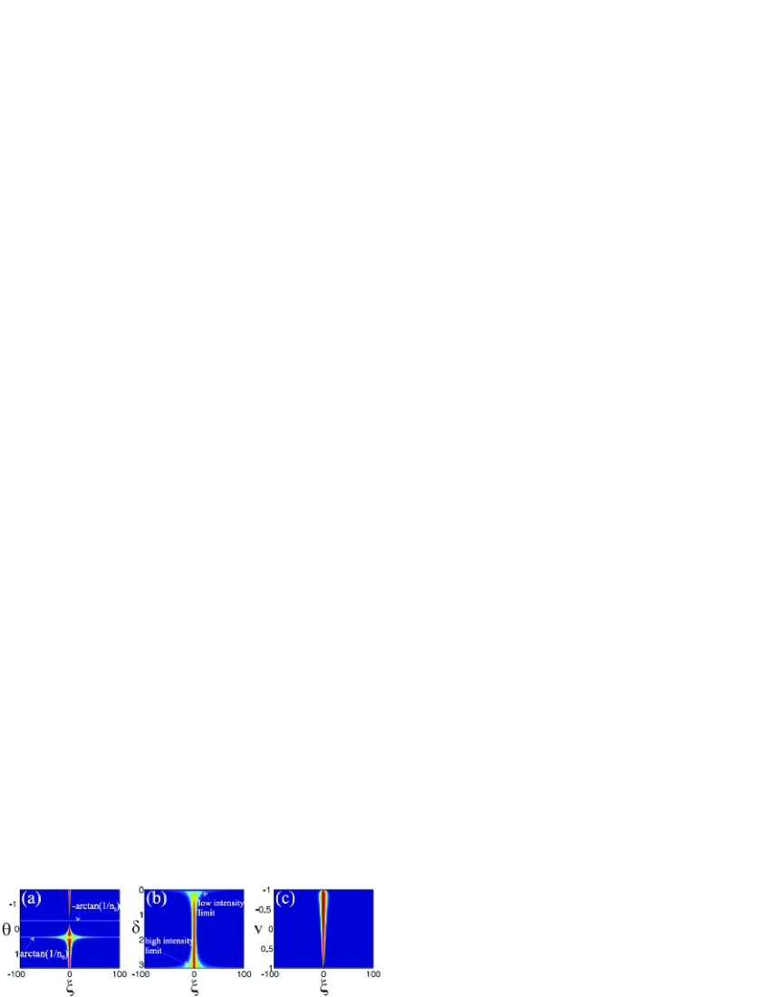
Figure 3: (Color online) Contour plots of the total intensity profile $I_{tot}=|f|^{2}+|b|^{2}$ for the STGS: (a) as a function of $\theta$, for $v=0$ and $\delta=\pi/2$ [note the divergence located at $\theta=\arctan(1/n_{0})$, and the vanishing intensity in correspondence of $\theta=-\arctan(1/n_{0})$], (b) as a function of $\delta$, for $\theta=1.3$ and $v=0$, and (c) as a function of $v$, for $\theta=1.3$ and $\delta=\pi/2$. In all cases $n_{0}=3$.

Our analytical solution is also confirmed by direct numerical integration of Eqs.(4-5), performed using a split-step Fourier method with a $4$th order Runge-Kutta algorithm. Figure 2(b,c) shows the propagation of a STGS with parameters $v=0$, $\theta=1.3$ and $\delta=\pi/2$, which lives in the center of the mixed bandgap displayed in Fig. 2(e), for a propagation of $\tau=7$. Fig. 2(b) shows that when the grating is absent ($\kappa=0$) the two components separate and do not interact, while Fig. 2(c) shows the undisturbed soliton propagation at zero relative velocity in presence of the spatiotemporal grating. Surprisingly, it is seen from the numerical simulations that quasi-adiabatic variations of $\theta$ during propagation, which thus change dynamically the background spatiotemporal grating, do not destroy the STGS, due to prompt pulse reshaping. This structural stability makes STGSs very attractive for storing, slowing down, converting and releasing optical energy in a controlled way, which may have profound implications for optical communications and quantum information processing [15].

In conclusion, in this Letter we have derived a set of CMEs that allow to describe nonlinear pulse propagation in a shallow grating with space-time variations of the refractive index. This structure generally possesses a bandgap in a rotated frequency-wavenumber space, where new GSs have been found analytically by solving an associated mMTM. Our formulation considerably generalizes the current theoretical understanding of periodic media to time-dependent refractive index. Future works will include the bifurcation and stability analysis of STGSs, and the natural extension of the theory to dispersive media.

We acknowledge financial support from the UK Engineering and Physical Sciences Research Council (EPSRC), Science Foundation Ireland (SFI) and the Irish Research Council for Science, Engineering and Technology (IRCSET).

References

[1] R. E. Slusher, B. J. Eggleton, Nonlinear photonic crystals (Springer, Berlin, 2003).
[2] W. Chen and D. L. Mills, Phys. Rev. Lett. 58, 160 (1987).
[3] D. N. Christodoulides and R. I. Joseph, Phys. Rev.
Lett. 62, 1746 (1989).
[4] A. B. Aceves and S. Wabnitz, Phys. Lett. A
141, 37 (1989).
[5] B. J. Eggleton et al., Phys. Rev. Lett. 76, 1627
(1996).
[6] F. R. Morgenthaler, IRE Trans. Microwave Theory Tech. MTT-6,
167 (1958).
[7] F. Biancalana et al., Phys. Rev. E 75,
046607 (2007).
[8] J. D. Jackson, Classical Electrodynamics (Wiley and Sons, New York, 1975).
[9] S. Wabnitz, Opt. Lett. 14, 1071 (1989).
[10] G. Van Simaeys et al., Phys. Rev. Lett. 92, 223902 (2004).
[11] S. Pitois, M. Haelterman and G. Millot, J. Opt. Soc. Am. B 19, 782 (2002).
[12] P. J. Morrison, Rev. Mod. Phys. 70, 467
(1998).
[13] K. A. Gorshkov and L. A. Ostrovsky, Physica D
3, 428 (1981).
[14] W. E. Thirring, Ann. Phys. (NY) 3, 91 (1958); E. A. Kuznetsov and A. V. Mikhailov, Teor. Mat. Fiz.
30, 193 (1970).
[15] M. D. Lukin and A. Imamoglu, Nature 413, 273
(2001); L. M. Duan et al., Nature 414, 413 (2001).