Aromatic emission from the ionised mane of the Horsehead nebula

Abstract

Context. This work is conducted as part of the “SPECPDR” program dedicated to the study of very small particles and chemistry in photo-dissociation regions with the Spitzer Space Telescope (SST).

Aims. We study the evolution of the Aromatic Infrared Bands (AIBs) emitters across the illuminated edge of the Horsehead nebula and especially their survival and properties in the HII region.

Methods. We present spectral mapping observations taken with the Infrared Spectrograph (IRS) at wavelengths 5.2-38 $\mu$m. The spectra have a resolving power of $\rm{\lambda/\Delta\lambda}$ = 64 - 128 and show the main aromatic bands, H₂ rotational lines, ionised gas lines and continuum. The maps have an angular resolution of 3.6-10.6″and allow us to study the nebula, from the HII diffuse region in front of the nebula to the inner dense region.

Results. A strong AIB at 11.3 $\mu$m is detected in the HII region, relative to the other AIBs at 6.2, 7.7 and 8.6 $\mu$m, and up to an angular separation of $\sim$ 20 ″(or 0.04 pc) from the ionisation front. The intensity of this band appears to be correlated with the intensity of the [NeII] at 12.8 $\mu$m and of H$\alpha$, which shows that the emitters of the 11.3 $\mu$m band are located in the ionised gas. The survival of AIB emitters in the HII region could be due to the moderate intensity of the radiation field (G₀ $\sim$ 100) and the lack of photons with energy above $\sim$25 eV. The enhancement of the intensity of the 11.3 $\mu$m band in the HII region, relative to the other AIBs can be explained by the presence of neutral PAHs.

Conclusions. Our observations highlight a transition region between ionised and neutral PAHs observed with ideal conditions in our Galaxy. A scenario where PAHs can survive in HII regions and be significantly neutral could explain the detection of a prominent 11.3 $\mu$m band in other Spitzer observations.

1 Introduction

Polycyclic Aromatic Hydrocarbons (PAHs) were proposed twenty years ago by Léger & Puget (1984) and Allamandola et al. (1985) to explain the infrared emission bands observed at 3.3, 6.2, 7.7, 8.6 and 11.3 $\mu$m. These emitters are an ubiquitous component of interstellar dust which has been observed with the Infrared Space Observatory (ISO) in a wide range of interstellar conditions (e. g. Boulanger et al., 1998a; Uchida et al., 2000). These aromatic infrared bands (AIBs) have already been observed in spectra attributed to HII regions (e. g. Peeters et al., 2002; Hony et al., 2001; Vermeij et al., 2002) but never with clear proof that their emitters are within the ionised gas rather than within an associated photodissociation region on the same line of sight. Moreover, several studies report the destruction of these emitters in the HII regions of M17 and the Orion Bar. In these regions, the strong radiation field is thought to be the main cause of this destruction (e. g. Kassis et al., 2006, and reference therein). In this paper, we use “PAHs” as a generic term in order to designate the emitters of the AIBs although the exact nature of these emitters is still a matter of debate.

Figure 1: H$\alpha$ map, in arbitrary units, obtained with the 0.9 m Kitt Peak National Observatory (KPNO) telescope (Pound et al., 2003). The contours show the areas observed with both IRS-SL (small area) and IRS-LL (large area).

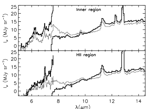
Figure 2: Average SL spectra obtained within the Inner and HII regions (see the contours of these two regions in Fig. 5) before (thick line) and after (thin line) correction of the residual emission (see § 2).

Dust grains can play an important role in the energetic balance of HII regions through photoelectric heating (Weingartner & Draine, 2001, and references therein). Since these processes are dominated by small grains, the presence of PAHs in HII regions has a strong impact on the physics of these objects.

In front of the western illuminated edge of the molecular cloud L1630, the visible plates are dominated by extended red emission due to the H$\alpha$ line emission emerging from the HII region IC434 (e. g. Louise, 1982). In the visible, the Horsehead nebula, also known as B33 (Barnard, 1919), emerges from the edge of L1630 as a dark cloud in the near side of IC434. The Horsehead nebula is a familiar object in astronomy and has been observed many times at visible, IR and submm wavelengths (Zhou et al., 1993; Abergel et al., 2003; Pound et al., 2003; Teyssier et al., 2004; Habart et al., 2005; Pety et al., 2005; Hily-Blant et al., 2005). IC434 and the Horsehead nebula are excited by the $\sigma$ Orionis star which is an O9.5V binary system (Warren & Hesser, 1977) with an effective temperature of $\sim$ 34 600 K (Schaerer & de Koter, 1997). L1630 is located at a distance of $\sim$400 pc. Assuming that $\sigma$ Orionis and the Horsehead are in the same plane perpendicular to the line of sight, the distance between them is $\sim$ 3.5 pc ($\sim$ 0.5°) which gives G₀ $\sim$ 100 (energy density of the radiation field between 6 and 13.6 eV in unit of Habing field, Habing, 1968) for the radiation field which illuminates the Horsehead nebula.

In this paper, we study the AIBs from IC434 in front of the Horsehead nebula observed with the Infrared Spectrograph (IRS; Houck et al., 2004) on board the Spitzer Space Telescope (Werner et al., 2004). The paper is organised as follows : in § 2, we present our IRS data and the data processing. In § 3, we show that IRS data confirm the description of the structure of the object from previous studies. In the following section (§ 4), we extract the typical spectrum of the HII region and study the location of the AIB emitters of this spectrum. We compare the HII region spectrum with the spectrum obtained in the inner region in § 5, and propose a scenario to explain the observed spectral variations in § 6. The survival of PAHs in the HII region is discussed in § 7. We conclude in § 8.

2 Observations & data reduction

The Horsehead nebula has been observed with IRS as a part of our “SPECPDR” program (Joblin et al., 2005) on 2004 October 2, and using the Short-High (SH), Long-High (LH) , Short-Low (SL) and Long-Low (LL) modules of the instrument. In this paper, we only present SL (5.2-14.5 $\mu$m, slit size: 57″ $\times$ 3.6″, R=64-128) and LL (14-38 $\mu$m, slit size: 168″ $\times$ 10.6″, R=64-128) observations. We used the “spectral mapping mode”. An observation is made of N_step= 23 (SL) or 25 (LL) steps of half the slit width in the direction perpendicular to the slit long axis. For the SL module, three observations were taken successively at three different positions on the sky in order to perform a complete mapping of the illuminated edge of the nebula. The resulting observed areas are shown in Fig. 1, overplotted on the H$\alpha$ map. The integration times were 14 and 60 s per pointing for the second (5.2-8.7 $\mu$m) and the first (7.4-14.5 $\mu$m) orders of SL, respectively, and 14 s per pointing for both orders of LL.

We have developed a pipeline which builds spectral cubes (two spatial dimensions and one spectral dimension) in a homogeneous way from the data (version S13) delivered by the Spitzer Science Center (SSC). We start from the BCD level. One integration corresponds to one BCD image. For each BCD image, we extract for all wavelengths an image of the slit which is projected on the sky. For each observation, made of N_step integrations, we build a spectral cube with N_x $\times$ N_y spatial pixels and $\rm{N_{w}}$ spectral pixels. We keep the same wavelength sampling as in the BCD images and the spatial grid has a pixel size of 2.5″  for LL and 0.9″  for SL (which corresponds to half the pixel size on the BCD images). Whenever we study the full spectral range, we also reproject the SL data on the LL grid.

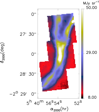
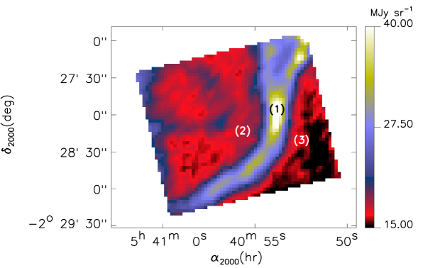
Figure 3: Maps of the Horsehead nebula at 11-11.5 $\mu$m (SL, left panel) and 20-21 $\mu$m (LL, right panel). The SL and LL maps have pixel size 0.9″and 2.5″, respectively. Positions of the spectra of Fig. 4 are shown on the LL map (right panel).

We identify and correct the bad pixels not flagged out in the SSC pipeline by median filtering on the combined N_step BCD images. The data are flux-calibrated in Jansky using the pipeline S13 conversion factors and the tuning coefficients given in the “fluxcon” table. Finally, we derive extended emission flux intensities by using the Slit Loss Correction Function due to the point-spread function overfilling the IRS slit (Smith et al., 2007). In the following, the LL data at 35-38 $\mu$m are not considered due to the strong decrease of sensitivity.

Only the HII region in front the Horsehead nebula presents nearly flat infrared emission and could have been used to define an off spectrum. Since the goal of this paper is precisely to study the emission emerging from the HII region, we did not subtract any off spectrum. The lack of such correction explains the discontinuity systematically found for all pixels between the first order and the second order parts of the SL spectra, together with a systematic decrease of the continuum with decreasing wavelength, down to negative values for wavelengths below $\sim$6 $\mu$m (Fig. 2). We find that for each pixel the amplitude of these effects does not depend on the detected emission, but appears strongly correlated with the non-zero emission detected in the interorder regions of the BCD images which in principle does not receive any incident photon. This non-zero emission does not depend on the emission in the order regions of the BCD images, but presents some correlation with the emission in the peakup region of the array. It could be a residual after the “droop” or the stray-light corrections (see the IRS data handbook). We estimate the amplitude of this residual in the order regions by extrapolating for each row the emission detected in the interorder regions, and subtract this residual from the BCD image. This subtraction is performed on the BCD image multiplied by the flat field image (taken in the calibration files delivered by the SSC), since we work in the hypothesis that the effects we want to correct are additive. Then, we divide the corrected BCD image by the flat field image. Finally, we build a corrected spectral cube using the algorithm described above. The correction only affects the shape of the continuum emission and does not change the amplitude of the spectral bands and lines. The discontinuity between the two orders of the SL spectra is strongly reduced (Fig. 2). However, we have to keep in mind that at that time the origin of the corrected effects is not known, therefore we must be cautious in the interpretation of the continuum emission.

3 The Horsehead as seen by IRS

Figure 4: Typical spectra obtained by combining SL and LL data for individual pixels (1) at the infrared peak position, (2) in the inner region of the Horsehead nebula behind the emission peak and (3) in front of the dense cloud in the HII region, as shown in the right panel of Fig. 3. Alternating thicknesses correspond to SL2, SL1, LL2 and LL1 orders. The dashed lines show the contribution of the zodiacal emission (see § 3).

Figure 3 gives an example of the spectral maps obtained from SL and LL observations. For all pixels within the SL field, we have a full spectrum from 5 to 35 $\mu$m (Fig. 4).

The zodiacal emission is computed using the SSC background estimator which is based on the COBE/DIRBE model (Kelsall et al., 1998). The dashed lines in Fig. 4 show the zodiacal contribution to our observations which is not simply the zodiacal emission at the date and sky coordinates of our observations. Indeed, the “dark” level subtracted from the data in the SSC pipeline is obtained without shutter by pointing a fixed area of the sky with faint infrared emission (RA = 268$\,\aas@@fstack{\circ}$96, DEC = 65$\,\aas@@fstack{\circ}$43) as explained in the IRS Data Handbook. This “dark” level will contain some zodiacal emission ($\sim$ 14 MJy sr^-1 at $\sim$ 18 $\mu$m). Therefore, the zodiacal contribution to our observations is the difference between the zodiacal emission at the time and the position of our observations and the zodiacal emission at the “dark” position. This zodiacal contribution does not vary across the observed area of the sky and is accurate to $\sim$14%³.

The spatial structure detected with IRS is comparable to the broad-band observations taken with ISOCAM (Abergel et al., 2003), but we now have the spectral information from 5 to 35 $\mu$m and better spatial resolution. Thanks to the edge-on geometry of this PDR, it is possible to perform spectral analysis of the emission in the HII region, the edge of the PDR and the inner region inside the PDR, separately. Three illustrative spectra for individual pixels are presented in Fig. 4:

• The first spectrum is taken at the infrared peak position and is typical for a PDR. It shows the main H₂ rotational lines (0-0 S(4) to S(0) at 6.9, 9.7, 12.3, 17.0 and 28.2 $\mu$m), the AIBs and continuum.

• The second spectrum is taken in the inner region behind the peak (to the east of the peak) and shows AIBs and H₂ emission lines with lower intensities since the emitting matter is located more deeply in the dense cloud.

• The third spectrum is taken in front of the illuminated surface in the HII region (to the west of the peak) and is dominated by fine structure lines of ionised species as expected for a HII region. It shows the following lines: [ArII] at 6.98 $\mu$m, [NeII] at 12.8 $\mu$m, [SIII] at 18.7 and 33.4 $\mu$m, [SiII] at 34.8 $\mu$m, but not the more excited lines: [NeIII] at 15.5 $\mu$m, [SIV] at 10.5 $\mu$m and [ArIII] at 9.0 $\mu$m. It also contains the 11.3 $\mu$m AIB.

Spectra (1) and (2) also present ionised lines which are likely emitted by the ionised medium surrounding the dense cloud. The continuum emission at wavelengths lower than $\sim$ 20 $\mu$m appears to be dominated by the zodiacal emission for the spectra (2) and (3).

In the following, we remove the zodiacal contribution from all spectra and focus our study on the SL spectra of the HII region which contains the 11.3 $\mu$m AIB. The study of the spectral properties around the peak position will be the subject of a forthcoming paper.

4 HII region spectrum

Figure 5: Emission maps of the 11.3 $\mu$m AIB, H₂ 0-0 S(2), [NeII] at 12.8 $\mu$m (as seen by IRS) and H$\alpha$ (Pound et al., 2003). The contours show the area defined as the HII region (west of the peak) and the inner region (east of the peak) in § 4 and § 5.

Figure 6: Mean spectra of the HII region (lower) and the inner region (upper) as defined in § 4 and § 5 and shown in Fig. 5. The [NeII] line at 12.8 $\mu$m is truncated for clarity. In the HII region spectrum, the broad feature at $\sim$ 10 $\mu$m is an artefact (see § 4 and Fig. 7). The zodiacal emission has been removed from these spectra (see § 3).

Fig. 5 shows emission maps of the 11.3 $\mu$m AIB (fitted with a lorentzian profile following Boulanger et al., 1998b), H₂ 0-0 S(2), [NeII] at 12.8 $\mu$m (both fitted with a gaussian profile) and H$\alpha$ obtained at the Kitt Peak National Observatory (KPNO) telescope by Pound et al. (2003) (Fig. 1). Both [NeII] and H${\alpha}$ are emitted by ionised gas. However, they cannot be used alone to define the HII region and exclude PDR emission which could be located on the same line of sight behind or in front of the ionised gas (with respect to us). We see in Fig. 5 that the H${\alpha}$ and [NeII] emissions do not peak at the same location due to projection effects and the difference of extinction efficiency since they emit at different wavelengths. We need a PDR tracer in order to exclude PDR emission. We use the H₂ 0-0 S(2) line at 12.3 $\mu$m since it is a good PDR tracer for this dense illuminated ridge (Habart et al., 2005), which is well detected in our data. Thus, we define the HII region as the area where $\rm{I}_{\rm{H}{\alpha}}$ $>$ 450 in arbitrary units and I(H₂ 0-0 S(2)) $<$ 6 10^-9 W m^-2 sr^-1 (detection limit due to the noise in individual spectra). We use H${\alpha}$ rather than [NeII] to trace the ionised gas since it is not affected by ionisation fraction effects. The contours of the HII region we have defined are shown in Fig. 5. The H${\alpha}$ emission in this HII region traces the ionised material in front of the Horsehead. In fact, the extinction due to this material on a line of sight is A_V $\sim$ 0.01-0.06, considering $\rm{n_{e}}$ $\sim$ $\rm{n_{H}\sim 100-350}$ cm^-3 (see appendix A), a depth of $\sim$0.1 pc for the Horsehead nebula (Habart et al., 2005) and $\rm{N_{H}/A_{V}}$ $\sim$ $\rm{1.87\,10^{21}\,cm^{-2}\,mag^{-1}}$ (Bohlin et al., 1978).

The average spectrum computed within this area (Fig. 6, lower spectrum) shows the [ArII] and [NeII] lines at 6.98 $\mu$m and 12.8 $\mu$m, respectively. A band is also detected at 11.3 $\mu$m with a surprisingly high intensity compared to the intensities of other AIBs at 6.2, 7.7 and 8.6 $\mu$m. Other bands seem necessary to account for the emission plateau between 11.3 and 13 $\mu$m. A broad emission feature is visible around 10 $\mu$m, however its amplitude is variable (Fig. 7) and depends strongly on the offset position from the center of the slit (i.e. on the position on the detector). We therefore conclude that this feature is mainly due to an artefact. On the other hand, the AIB at 11.3 $\mu$m is real since it appears everywhere in the HII region with a strong amplitude, as shown in Fig. 7.

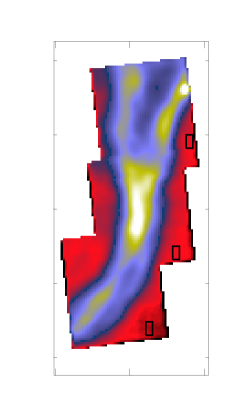
Figure 7: Spectra from three areas (small black rectangles) shown on the 11-11.5 $\mu$m map (top, middle and lower panels correspond to the north, the central and the south area, respectively). The zodiacal emission has been subtracted (see § 3). For clarity, the [NeII] line is truncated. The broad feature at $\sim$ 10 $\mu$m in the spectrum of the top panel is an artefact (see § 4).

A method to check whether the 11.3 $\mu$m emitters are located in the ionised gas is to look for spatial correlation between the 11.3 $\mu$m AIB and the ionised gas lines emission in the HII region. The figure 8 presents the $11.3\,\mu$m AIB vs [NeII] and vs H$\alpha$ correlation diagrams for pixels of the HII region. The computed [NeII] line intensity is not affected by a possible contribution of the 12.7 $\mu$m AIB, since our spectral decomposition takes into account this AIB. We see that the $11.3\,\mu$m AIB intensity is correlated with both the [NeII] and H$\alpha$ ones which shows that the observed correlation is not dominated by systematic effects in the IRS data. The correlation coefficients are 0.56 and 0.63 for $11.3\,\mu$m AIB vs [NeII] and $11.3\,\mu$m AIB vs H$\alpha$, respectively. Note that we have only considered the points within the 3$\sigma$ limit with respect to the linear fitting (dashed lines in Fig. 8). The relatively low values of the correlation coefficients are due to systematic effects on the IRS computed maps (striping, Fig. 5) and to the fact that the relationship between the ionised gas lines intensity and the AIBs intensity is not systematically linear.

At least about half the 11.3 $\mu$m emitters on the line of sight should be located in the ionised gas in front of the Horsehead nebula where the H$\alpha$ and [NeII] emissions rise, since the two correlations range from $\sim$ 2.5 to $\sim$ 4.5 10^-8 W m^-2 sr^-1 for the 11.3 $\mu$m AIB intensity. A typical Cirrus spectrum has been estimated by Flagey et al. (2006) from ISOCAM data (Fig. 9, upper spectrum). It presents a shape comparable to the HII spectrum, except for the 6.2 $\mu$m AIB which indicates that the contribution of Cirrus emission does not dominate the detected HII spectrum. In any case, the contribution of Cirrus should be comparable for the HII region and inner region spectra (as defined in the next section), and cannot affect our conclusions based on spectral variations between these two spectra.

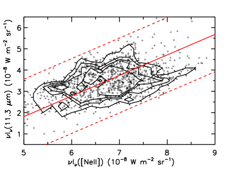
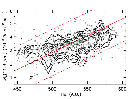
Figure 8: Relationships between the [NeII], H$\alpha$ and $11.3\,\mu\rm{m}$ for pixels of the HII region (defined in § 4 and shown in Fig. 5). Contours are histograms of the point densities. The red straight lines are linear fits to the data. The red dashed lines are the 3$\sigma$ limit with respect to the linear fitting.

Figure 9: Cirrus spectrum observed with ISOCAM (Flagey et al., 2006) and HII region spectrum as defined in § 4 convolved with a gaussian yielding a resolving power of 40, comparable to ISOCAM-CVF. The 9-10.5 $\mu$m range is suppressed since it contain an artefact (§ 4).

5 Comparison with the inner region spectrum

As for the HII region (§ 4), we define an inner region where $\rm{I}_{\rm{H}{\alpha}}$ $<$ 135 in arbitrary units and $\rm{I}_{\nu,11-11.5\mu\rm{m}}$ $<$ 15 MJy sr^-1 in order to avoid the bright infrared filament (Fig. 5) were the [NeII] emission peaks due to projection effets. The average spectrum computed within this area (Fig. 6, upper spectrum) shows the 0-0 S(3)-9.7 $\mu$m and 0-0 S(2)-12.3 $\mu$m H₂ rotational lines, the AIBs at 6.2, 7.7, 8.6 and 11.3 $\mu$m and the [NeII] line at 12.8 $\mu$m. The 0-0 S(5)-6.9 $\mu$m H₂ and [ArII] (6.98 $\mu$m) lines are blended.

The presence of [NeII] and [ArII] lines indicates that this spectrum contains ionised gas emission and could contain AIBs emitted in the background and foreground ionised medium. However, such a contribution from HII region AIBs will not change the conclusions of our analysis of the spectral variations that we study in the following.

The relative intensity of the AIBs presents striking differences between the HII region and inner region spectra (Fig. 6). While the intensity of the 11.3 $\mu$m band is comparable, the 6.2, 7.7 and 8.6 $\mu$m bands present a spectacular decrease in the HII region (more than a factor 2-3). The 6.2 and 7.7 $\mu$m bands are attributed to C-C stretching mode, the 8.6 $\mu$m band to in-plane C-H bending modes, and the 11.3 $\mu$m band to C-H out-of-plane bending mode. In the following section, we study the different processes which could explain such spectral variation of the 6-9 $\mu$m / 11.3 $\mu$m ratio.

6 Interpretation of the spectral properties

6.1 Hydrogenation state

Hydrogenation state of PAHs can be traced by relative intensities of the 11.3, 12, 12.7 and 13.6 $\mu$m bands (e. g. Schutte et al., 1993) which are C-H out-of-plane bending modes with one, two, three and four H atoms on the same aromatic ring, respectively (e. g. Léger & Puget, 1984; Hony et al., 2001). Both inner region and HII region spectra (Fig. 6) present an 11.3 $\mu$m band and an emission plateau between 11.3 and 13 $\mu$m above the continuum, which can be attributed to hydrogenated PAHs (high hydrogenation coverage of PAHs has already been reported in HII regions and PDRs, e. g. Vermeij et al., 2002; Hony et al., 2001). Moreover the intensity of the 11.3 $\mu$m band compared to the plateau does not present any strong variation between the two spectra, which indicates that the hydrogenation states are comparable. We conclude that hydrogenation effects are likely not the main process which could explain the difference in the 6-9 $\mu$m / 11.3 $\mu$m ratio between the two spectra.

6.2 Size distribution

Using the model of Verstraete et al. (2001), we find that the emission ratio of 6-9 $\mu$m / 11.3 $\mu$m is reduced by a factor of 3 only if the size distribution contains exclusively PAHs bigger than 10³ C atoms ($\sim$ 30 Å) in the HII region while it is a classical size distribution (mean size $\sim$ 6 Å, e.g. Bakes & Tielens, 1994) in the inner region. Then, we conclude that a change in the size distribution due to destruction of smallest species cannot explained the 6-9 $\mu$m / 11.3 $\mu$m ratio variation.

6.3 Charge state

Theoretical (e. g. Langhoff, 1996; Bakes et al., 2001a, b; Bauschlicher, 2002) and experimental (e. g. Szczepanski et Vala, 1993) works show that the charge state of PAHs has a strong impact on the 6-9 $\mu$m / 11.3 $\mu$m ratio. Neutral PAHs emit significantly less at 6-9 $\mu$m than at 11-13 $\mu$m with respect to charged ones (both anions and cations). The inner region spectrum which comes from neutral gas presents a high value of the 6-9 $\mu$m / 11.3 $\mu$m ratio, which can be explained by charged PAHs (anions or cations). On the contrary, the low value of the 6-9 $\mu$m / 11.3 $\mu$m ratio in the HII region spectrum can be explained by the presence of neutral PAHs. The spectra extracted from ISOCAM observations (4-16 $\mu$m) of NGC7023 present comparable relative intensity variations attributed to charge effects (Rapacioli et al., 2005). Our spectra from the HII region and the inner region (Fig. 6) could therefore be attributed to PAH⁰ and PAH⁺, respectively.

The charge state of PAHs is mainly determined by the balance between photoionisation and recombination rates of electrons (Weingartner & Draine, 2001; Bakes & Tielens, 1994) which is generally described by the ratio of the UV intensity to the electronic density, G₀/n_e. The presence of positively charged PAHs in the inner region can be explained by (1) the presence of UV photons which efficiently ionise the PAHs and (2) a lack of free electrons for the recombination (n_e/n_H $\sim$ [C]/[H] $\sim$ 10^-4, C⁺ being the main provider of electrons in the PDR).

For the HII region, we use version 05.07 of Cloudy (Ferland et al., 1998) in order to derive a quantitative estimate of the charge state of PAHs (van Hoof et al., 2004; Weingartner & Draine, 2001) in a fully (n_e $\sim$ n_H) ionised medium. We perform a simple model with an incident radiation field defined for an O9.5V star of the Costar catalogue (Schaerer & de Koter, 1997) and located at 3.5 pc. The gas is taken to be at T = 7500 K (Ferland, 2003) and with n_e $\sim$ 100-350 cm^-3 (see appendix A). For PAHs with radius from 4.5 to 10.5 $\AA$ and distributed as n(a) $\propto$ a^-3.5 (Bakes & Tielens, 1994), we obtain a mean charge of 0.55 - 0.75 electron per PAH, corresponding to a fraction of neutral PAHs in the HII region of 25 - 45%. Moreover, the 6-9 $\mu$m / 11.3 $\mu$m ratio of the HII region spectrum is in agreement with those predicted by the emission model of Bakes et al. (2001a) for such a charge distribution. We conclude that the HII region spectrum can be explained by a mixture of neutral and anionic PAHs.

7 PAHs survival in the HII region

The 11.3 $\mu$m band is observed in the HII region up to a distance of $\sim$ 20 ″(or 0.04 pc) from the ionisation front (see for instance Fig. 5). This distance can be translated to a lower limit of the survival time of the emitters equal to $\sim$ 5 10³ years when considering that the gas just ionised at the ionisation front expands freely in the HII region at the sound speed c_s = $\sqrt{\frac{\gamma\rm{kT}}{\mu\rm{m_{H}}}}$ $\sim$ 10 km s^-1 for T = 7500 K, $\mu$ = 0.7 and $\gamma$ = 5/3.

We have seen in § 3 that in the HII region, all species with an ionisation potential (IP) lower or equal than that of [SIII] (IP=23.34 eV) are detected while species with IP higher or equal than that of [ArIII] (IP=27.63 eV) are not detected. Thus, the incident radiation field in the HII region contains UV photons with energy up to $\sim$ 25 eV. Thus, some aromatic emitters can survive to a radiation field with G₀ $\sim$ 100 and photons up to $\sim$ 25 eV. For comparison, in more highly excited HII regions such as the Orion Bar, the radiation field is more intense (G₀ larger than 10⁴) and also harder since the exciting star is an O6 ($\rm{\theta^{1}\,Ori\,C}$, e.g. Kassis et al., 2006; Allers et al., 2005) with $\rm{T_{eff}}\,\sim\,44000\,K$. There, PAHs are destroyed on time scales lower than 1000 years (Kassis et al., 2006).

It must be emphasized that the presence of AIB emitters in the ionised gas could be related to the continuous injection of “fresh” matter due to photoevaporation of the Horsehead.

8 Conclusion

Our main observational result is the detection of a strong 11.3 $\mu$m emission band in the HII region facing the Horsehead nebula. The spectral imaging capabilities of IRS allow us to show that the integrated intensity of the $11.3\,\mu\rm{m}$ AIB is correlated with those of the [NeII] line and H$\alpha$ in the HII region. Moreover the spectral variations of the AIB spectrum is clearly spatially correlated with the variations of physical conditions between the PDR and the HII region. Thus, to our knowledge, this is the first time that we detect the presence of AIB emitters in ionised gas. Consequently, the $11.3\,\mu\rm{m}$ emitters are not efficiently destroyed by the incident UV photons which have an energy below $\sim$ 25 eV as suggested by the detected ionised species. The survival of PAHs in the HII region could be due to the moderate intensity of the radiation field (G₀ $\sim$ 100) and the lack of photons above $\sim$ 25 eV, compared to more highly excited HII regions (in terms of intensity and hardness), where PAHs can be destroyed on time scales lower than 1000 years (Kassis et al., 2006). It could also be related to the continuous photoevaporation of the Horsehead nebula which bring “fresh” matter into the ionised gas.

The enhancement of the intensity of the 11.3 $\mu$m band in the HII region, relative to the other AIBs, can be explained by the presence of neutral PAHs. Our modelling of the charge state of PAHs with Cloudy confirms that the HII region should contain a significant amount of neutral PAHs. On the contrary, PAHs from the inner region must be positively charged. Variations of the size distribution of PAHs could also affect the 6-9 $\mu$m / 11.3 $\mu$m ratio (e. g. Verstraete et al., 2001) but with a lower amplitude than charge state variations.

In galaxies, the presence of neutral PAHs has been suggested by Kaneda et al. (2005) to explain the prominent emission feature at 11.3 $\mu$m compared to the 6.2, 7.7 and 8.6 $\mu$m features observed with Spitzer in several elliptical galaxies. The present IRS observations of the Horsehead nebula thus provide a textbook example in our Galaxy of the transition region between ionised and neutral PAHs and allow to derive a physical scenario in order to interpret extra-galactic spectra.

Appendix A Determination of the electronic density

The electronic density in the HII region is estimated using the intensity ratio of the [SIII] lines at 18.7 and 33.4 $\mu$m. These two lines are fitted with gaussian profiles in order to compute their integrated intensities for all pixels in the HII region (see § 4 and Fig. 5). The mean intensities are I([SIII], 19 $\mu$m) = 2.69 $\pm$ 0.11 10^-8 W m^-2 sr^-1 and I([SIII], 33 $\mu$m) = 3.91 $\pm$ 0.42 10^-8 W m^-2 sr^-1. Error bars include the calibration uncertainties (absolute stellar model (1 $\sigma$ = 3%), the repeatability ($\sim$ 3%) and the uncertainty of the calibration at 33.4 $\mu$m ($\sim$ 10%)). We have I([SIII], 19 $\mu$m) / I([SIII], 33 $\mu$m) = 0.69 $\pm$ 0.08. Consequently, using atomic constants from Galavis et al. (1995) and Mendoza & Zeippen (1982) and assuming a gas temperature of 7500 K (Ferland, 2003), we derive an electronic density n_e $\sim$ 100-350 cm^-3.

References

- Abergel et al. (2003) Abergel, A., Teyssier, D., Bernard, J.P. et al., 2003, A&A, 410, 577
- Allamandola et al. (1985) Allamandola, L. J., Tielens, A. G. G. M. & Barker, J. R., 1985, ApJL, 290, L25
- Allers et al. (2005) Allers, K. N., Jaffe, D. T., Lacy, J. H et al., 2005, ApJ, 630, 368
- Anthony-Twarog (1982) Anthony-Twarog, B. J., 1982, AJ, 87, 1213
- Bakes et al. (2001a) Bakes, E. L. O., Tielens, A. G. G. M., Bauschlicher, Charles W., Jr., 2001a, ApJ, 556, 501
- Bakes et al. (2001b) Bakes, E. L. O., Tielens, A. G. G. M., Bauschlicher, Charles W., Jr. et al., 2001b, ApJ, 560, 261
- Bakes & Tielens (1994) Bakes, E. L. O. & Tielens, A. G. G. M., 1994, ApJ, 427, 822
- Barnard (1919) Barnard, E. E., 1919, ApJ, 49, 1
- Bauschlicher (2002) Bauschlicher, Charles W., Jr., 2002, ApJ, 564, 782
- Bohlin et al. (1978) Bohlin, R. C., Savage, B. D., Drake, J. F., 1978, ApJ, 224, 132-142
- Boulanger et al. (1998a) Boulanger, F., Abergel, A., Bernard, J. P. et al., 1998a, ASPC, 132, 15
- Boulanger et al. (1998b) Boulanger, F., Boisssel, P., Cesarsky, D. et al., 1998b, A&A, 339, 194
- Ferland (2003) Ferland, G. J., 2003, ARA&A, 41, 517
- Ferland et al. (1998) Ferland, G. J., Korista, K. T., Verner, D. A. et al., 1998, PASP, 110, 761
- Flagey et al. (2006) Flagey, N., Boulanger, F., Verstraete, L. et al., 2006, A&A, 453, 969
- Galavis et al. (1995) Galavis, M. E., Mendoza, C., Zeippen, C. J., 1995, A&AS, 111, 347
- Habart et al. (2005) Habart, E. , Abergel, A., Walmsley, C. et al., 2005, A&A, 437, 177
- Habing (1968) Habing, H. J., 1968, Bull. Astr. Netherlands, 19, 421
- Hily-Blant et al. (2005) Hily-Blant, P., Teyssier, D., Philipp, S. et al., 2005, A&A, 440, 909
- Hony et al. (2001) Hony, S., Van Kerckhoven, C., Peeters, E. et al., 2001, A&A, 370, 1030
- Houck et al. (2004) Houck, J. R., Roellig, T. L., van Cleve, J. et al., 2004, ApJS, 154, 18
- Joblin et al. (2005) Joblin, C., Abergel, A., Bernard, J.-P. et al., 2005, IAUS, 231, 153
- Kaneda et al. (2005) Kaneda, H., Onaka, T., Sakon, I., 2005, ApJ, 632L, 83
- Kassis et al. (2006) Kassis, Marc, Adams, Joseph D., Campbell, Murray F., 2006, ApJ, 637, 823
- Kelsall et al. (1998) Kelsall, T., Weiland, J. L., Franz, B. A. et al., 1998, ApJ, 508, 44
- Langhoff (1996) Langhoff, S. R, 1996, J. Phys. Chem., 100, 2819
- Léger & Puget (1984) Léger A. & Puget J.L., 1984, A&A, 137, L5
- Louise (1982) Louise, R., 1982, Ap&SS, 85, 405
- Peeters et al. (2002) Peeters E., Martín-Hernández N. L., Damour F. et al., 2002, A&A, 381, 571
- Pety et al. (2005) Pety, J., Teyssier, D., Fossé, D. et al., 2005, A&A, 435, 885
- Mendoza & Zeippen (1982) Mendoza, C., Zeippen, C. J., 1982, MNRAS, 199, 1025
- Pound et al. (2003) Pound, Marc W., Reipurth, Bo, Bally, John, 2003, AJ, 125, 2108
- Rapacioli et al. (2005) Rapacioli, M., Joblin, C., Boissel, P., 2005, A&A, 429, 193
- Schaerer & de Koter (1997) Schaerer, D. & de Koter, A., 1997,A&A, 322, 598
- Schutte et al. (1993) Schutte, W. A., Tielens, A. G. G. M., Allamandola, L. J., 1993, ApJ, 415, 397
- Smith et al. (2007) Smith, J.D., Draine, B.T., Dale, D.A. et al., 2007, ApJ, 656, 770-791
- Szczepanski et Vala (1993) Szczepanski Jan et Vala Martin, 1993, ApJ, 414, 646
- Teyssier et al. (2004) Teyssier, D., Fossé, D., Gerin, M. et al., 2004, A&A, 417 ,135
- Uchida et al. (2000) Uchida, K. I., Sellgren, K., Werner, M. W. et al., 2000, ApJ, 530, 817
- van Hoof et al. (2004) van Hoof, P. A. M., Weingartner, J. C., Martin, P. G. et al, 2004, MNRAS, 350, 1330
- Vermeij et al. (2002) Vermeij, R., Peeters, E., Tielens, A. G. G. M. et al., 2002, A&A, 382, 1042
- Verstraete et al. (2001) Verstraete, L., Pech, C., Moutou, C. et al., 2001, A&A, 372, 981
- Warren & Hesser (1977) Warren, W. H., Jr.& Hesser, J. E., 1977, ApJS, 34, 115
- Weingartner & Draine (2001) Weingartner, Joseph C. & Draine, B. T., 2001, ApJS, 134, 263
- Werner et al. (2004) Werner, M. W., Roellig, T. L., Low, F. J. et al, 2004, ApJS, 154, 1
- Zhou et al. (1993) Zhou, S., Jaffe, D. T., Howe, J. E. et al., 1993, ApJ, 419, 190