Abstract

In this article we review our work on the dynamics and decoherence of electron and hole spins in single and double quantum dots. The first part, on electron spins, focuses on decoherence induced via the hyperfine interaction while the second part covers decoherence and relaxation of heavy-hole spins due to spin-orbit interaction as well as the manipulation of heavy-hole spin using electric dipole spin resonance.

Chapter 0 Electron and hole spin dynamics and decoherence in quantum dots

1 Introduction

The Loss-DiVincenzo proposal[1] to use the spin of a single electron confined in a quantum dot as a qubit for quantum computation has triggered significant interest in the dynamics and control of single spins in quantum dots. This has led to numerous exciting experimental achievements, among them the realization of single electrons in single dots [2, 3] as well as double dots [4, 5, 6], the implementation of single-spin read out[7, 8], the demonstration of the $\sqrt{\mathrm{SWAP}}$ operation via pulsed exchange interaction[9] and the measurement of single-spin ESR [10]. For a detailed account of the progress in implementing the Loss-DiVincenzo proposal, see the extensive reviews in Refs. 11 and 12.

On the theoretical side, one focus was, and still is, the investigation of the decoherence induced by the nuclei in the host material via the hyperfine interaction. The first part of this review article is devoted to the discussion of the rich spin dynamics that results from the hyperfine interaction. We first give an introduction to hyperfine interaction in quantum dots (Sec. 2). Subsequently, we discuss dynamics under the influence of hyperfine interaction for the case of a single spin in a single dot (Sec. 3) and for a double dot with one electron in each dot (Sec. 4). To conclude the part about hyperfine interaction, we discuss the idea of narrowing the nuclear spin state in order to increase the spin coherence time (Sec. 5).

The second part of the article is devoted to the dynamics and the manipulation of heavy-hole spins in quantum dots. The motivation to study hole spins comes from the fact that the valence band has $p$-symmetry and thus the hyperfine interaction with lattice nuclei for holes is suppressed in comparison to that of the conduction band electrons. As a consequence, the main interest for hole spin dynamics is the relaxation and decoherence due to spin-orbit interaction and we discuss this in Sec. 6. The next task towards using hole spins as qubits for quantum computation is of course the coherent manipulation of single hole spins. A potentially powerful method to achieve coherent manipulation of spins is electric dipole spin resonance (EDSR). An analysis of EDSR for heavy holes in quantum dots will be presented in Sec. 7.

2 Hyperfine interaction for electrons in quantum dots

In this part of the article concerning electron spin decoherence we assume that the orbital level spacing is much larger than the typical energy scale of the hyperfine interaction. This is the case in typical lateral quantum dots containing single electrons and allows one to write an effective hyperfine Hamiltonian $H_{\mathrm{hf}}$ for a single electron confined to the quantum-dot orbital ground state $\psi_{0}$

$$H_{\mathrm{hf}}=\mathbf{h}\cdot\mathbf{S},\,\,\,\mathbf{h}=A\nu\sum_{k}|\psi_{0}(\mathbf{r}_{k})|^{2}\mathbf{I}_{k},$$ (1)

where $\mathbf{S}$ is the spin-1/2 operator for a single electron and $\mathbf{I}_{k}$ is the spin operator for the nuclear spin at lattice site $k$, while $\nu$ is the volume of the crystal unit cell and $A$ is the hyperfine coupling strength. For GaAs, which is mostly used for the fabrication of lateral dots, the average hyperfine coupling strength weighted by the natural abundance of each isotope is $A\approx 90\mu eV$ [13]. In Fig. 1 the hyperfine coupling of the electron spin in a lateral double quantum dot is illustrated.

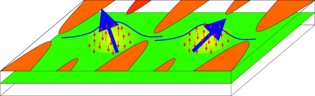
Figure 1: A double quantum dot. Top-gates are set to a voltage configuration that confines the electrons in the two-dimensional electron gas (green) to quantum dots (yellow). The blue line indicates the envelope wave function of the electron (blue arrow). The hyperfine interaction with a particular nuclear spins (red arrows) is proportional to the envelope wave function squared at the position of the nuclei. Thus the nuclear spins in the center are drawn bigger since they couple stronger to the electron spin.

The electron spin dynamics under $H_{\mathrm{hf}}$ have been studied under various approximations and in different parameter regimes. For an extensive overview, see reviews in Refs. 11, 14 and 15. Here, we briefly mention parts of this study before we focus on a few cases of special interest. The first analysis of electron spin dynamics under $H_{\mathrm{hf}}$ in this context showed that the long-time longitudinal spin-flip probability is $\sim 1/p^{2}N$ [16], i.e., this probability is suppressed in the limit of large nuclear spin polarization $p$ and large number $N$ of nuclear spins in the dot. An exact solution for the case of full polarization ($p=1$) gives, for both transverse and longitudinal electron spin components, a long-time power law decay $\sim 1/t^{3/2}$ by a fraction $\sim 1/N$ on a timescale of $\tau\sim\hbar N/A\sim 1\mu s$ (for a GaAs dot with $N\sim 10^{5}$)[17]. The fact that this exact solution shows a non-exponential decay demonstrates the non-Markovian behavior of the nuclear spin bath. For non-fully polarized systems $p<1$ and in the limit of large magnetic fields (or high polarization $p\gg 1/\sqrt{N}$), the transverse electron spin undergoes a Gaussian decay[17, 18] on a timescale $\tau\sim\hbar\sqrt{N}/A\sqrt{1-p^{2}}$ ($\tau\sim 5ns$ for GaAs with $p\ll 1$ and $N\sim 10^{5}$)[19]. This Gaussian decay can be reversed using a spin-echo sequence or by preparing the nuclear spin system in an eigenstate of $h_{z}$ [19].

Several methods to prepare the nuclear spin system have recently been suggested [20, 21, 22] and we discuss one of these methods [21] in Sec. 5. Once the nuclear spin system is prepared in an eigenstate, the electron spin coherence is on one hand limited by dynamics in the nuclear spin system driven by the dipole-dipole interaction for which a worst case estimate [21] gives $\sim 100\mu s$ and on the other hand, even for an eigenstate of $h_{z}$, there is decoherence due to the flip-flop dynamics which can be important at times $\sim\hbar N/A\sim 1\mu s$ (or less, depending on the size of the electron Zeeman splitting). For the decay of nuclear spin polarization experiments suggest timescales up to tens of seconds[23, 24, 25, 26] and hysteretic behavior of the nuclear spin polarization with respect to the external magnetic field has been observed [27]. Further, measurements of the transport current in the so-called spin-blockade regime [28] revealed hysteretic behavior with respect to the magnetic field [29, 23] and bistable behavior in time[23], which is attributed to a bistability in the nuclear spin polarization. Further, very recent experiments suggest a strong dependence of the nuclear field correlation time depending on whether an electron is present in the dot or not and thus hyperfine mediated nuclear spin flips are a possible mechanism for nuclear spin diffusion[24]. This last mechanism has been estimated to lead to fluctuations of nuclear spin polarization on a timescale of $\sim 100\mu s$[21].

3 Single-electron spin decoherence

In this section we look in more detail at hyperfine-induced decoherence for a single spin in a quantum dot in the regime of large Zeeman splitting $\epsilon_{z}=g\mu_{B}b_{z}$ (due to an externally applied magnetic field $b_{z}$). If $\epsilon_{z}$ is much larger than $\sigma=[\mathrm{Tr}\{\rho_{I}(h_{z}-h_{0})^{2}\}]^{1/2}$, with $h_{0}=\mathrm{Tr}\{\rho_{I}h_{z}\}$ (where $\rho_{I}$ is the density matrix of the nuclear spin system), we may neglect the transverse term $S_{\bot}\cdot h_{\bot}$ and find that the Hamiltonian is simply

$$H_{0}=(\epsilon_{z}+h_{z})S_{z}.$$ (2)

This Hamiltonian just induces precession around the $z$-axis with a frequency that is determined by the eigenvalue $h_{z}^{n}$ of $h_{z}$, where $h_{z}|n\rangle=h_{z}^{n}|n\rangle$. For a large but finite number of nuclear spins ($N\sim 10^{5}$ for lateral GaAs dots) the eigenvalues $h_{z}^{n}$ are Gaussian distributed (due to the central limit theorem) with mean $h_{0}$ and variance $\sigma\approx\hbar A/\sqrt{N}$ [19]. Calculating the dynamics under $H_{0}$ (which is valid up to a timescale of $\sim\epsilon_{z}/\sigma^{2}\sim 1\mu s$, where the transverse terms become relevant) leads to a Gaussian decay of the transverse electron spin state $|+\rangle=(|\uparrow\rangle+|\downarrow\rangle)/\sqrt{2}$ [19]:

$$C^{0}_{++}(t) = \frac{1}{\sqrt{2\pi}\sigma}\int^{\infty}_{-\infty}dh_{z}^{n}e^{\left(-\frac{(h_{z}^{n}-h_{0})^{2}}{2\sigma^{2}}\right)}|\langle n|\otimes\langle+|e^{(-iH_{0}t)}|+\rangle\otimes|n\rangle|^{2}$$ (3)

$$= \frac{1}{2}+\frac{1}{2}e^{\left(-\frac{t^{2}}{2\tau^{2}}\right)}\cos\left[(\epsilon_{z}+h_{0})t\right];\,\,\,\,\,\tau=\frac{1}{\sigma}=\sqrt{\frac{N}{1-p^{2}}}\frac{2\hbar}{A}.$$

Here again, $p$ denotes the polarization and for an unpolarized GaAs quantum dot with $N\sim 10^{5}$ we find $\tau\sim 5ns$. Applying an additional ac driving field with amplitude $b$ along the $x$-direction leads to single-spin ESR. Assuming again that $\epsilon_{z}\gg\sigma$, we have the Hamiltonian

$$H_{\mathrm{ESR}}=H_{0}+b\cos(\omega t)S_{x}.$$ (4)

In a rotating-wave approximation (which is valid for $(b/\epsilon_{z})^{2}\ll 1$) the decay of the driven Rabi oscillations is given by[30]

$$C^{\mathrm{ESR}}_{\uparrow\uparrow}(t)\sim 1-C+\sqrt{\frac{b}{8\sigma^{2}t}}\cos\left(\frac{b}{2}t+\frac{\pi}{4}\right)+\mathcal{O}\left(\frac{1}{t^{3/2}}\right),$$ (5)

for $t\gtrsim\mathrm{max}\left(1/\sigma,1/b,b/2\sigma^{2}\right)$ and $\epsilon_{z}+h_{0}-\omega=0$. Here, $C^{\mathrm{ESR}}_{\uparrow\uparrow}(t)$ is defined in the same way as $C^{0}_{++}(t)$ in Eq. (3). The time-independent constant is given by $C=\exp(b^{2}/8\sigma^{2})\mathrm{erfc}(b/\sqrt{8}\sigma)\sqrt{2\pi}b/8\sigma$. The two interesting features of the decay are the slow ($\sim 1/\sqrt{t}$) power law and the universal phase shift of $\pi/4$. The fact that the power law already becomes valid after a short time $\tau\sim 15ns$ (for $b\approx\sigma$) preserves the coherence over a long time, which makes the Rabi oscillations visible even when the Rabi period is much longer than the timescale $\tau\sim 15ns$ for transverse spin decay. Both the universal phase shift and the non-exponential decay have recently been observed in experiment [30]. In order to take corrections due to the transverse terms $S_{\bot}\cdot h_{\bot}$ into account, a more elaborate calculation is required. The Hamiltonian with flip-flop terms (but without a driving field) takes the form

$$H_{\mathrm{ff}}=H_{0}+\frac{1}{2}(S_{+}h_{-}+S_{-}h_{+}).$$ (6)

In Ref. 19 a systematic calculation taking into account these so-called flip-flop terms was performed using a generalized master equation, valid in the limit of large magnetic field or large polarization. This calculation shows that even for an eigenstate of $h_{z}$, for which the Gaussian decay in Eq. (3) vanishes, the electron spin undergoes nontrivial non-Markovian decay on a timescale $\hbar N/A\sim 10\mu s$.

Other calculations [31, 32, 33] give microsecond timescales for the electron spin decoherence due to electron-nuclear spin flip-flops processes. The results in Ref. 31 suggest that also the decoherence due to dynamics in the nuclear spin system via electron mediated nuclear dipole-dipole interaction is suppressed by a spin echo and thus that the spin-echo decay time may be considerably different from the (not ensemble averaged) free-induction decay.

4 Singlet-triplet decoherence in a double quantum qot

We now move on to discuss hyperfine induced decoherence in a double quantum dot. The effective Hamiltonian in the subspace of one electron on each dot is best written in terms of the sum and difference of electron spin and collective nuclear spin operators: $\mathbf{S}=\mathbf{S}_{1}+\mathbf{S}_{2},\delta\mathbf{S}=\mathbf{S}_{1}-\mathbf{S}_{2}$ and $\mathbf{h}=\frac{1}{2}(\mathbf{h}_{1}+\mathbf{h}_{2}),\delta\mathbf{h}=\frac{1}{2}(\mathbf{h}_{1}-\mathbf{h}_{2})$:

$$H_{\mathrm{dd}}(t)=\epsilon_{z}S_{z}+\mathbf{h\cdot S}+\delta\mathbf{h\cdot}\delta\mathbf{S}+\frac{J}{2}\mathbf{S\cdot S}-J.$$ (7)

Here, $J$ is the Heisenberg exchange coupling between the two electron spins. Similar to the single-dot case, we assume that the Zeeman splitting is much larger than $\langle\delta\mathbf{h}\rangle_{\mathrm{rms}}$ and $\langle\mathbf{h}_{i}\rangle_{\mathrm{rms}}$, where $\langle\mathcal{O}\rangle_{\mathrm{rms}}=[\mathrm{Tr}\{\rho_{I}(\mathcal{O}-\langle\mathcal{O}\rangle)^{2}\}]^{1/2}$ is the root-mean-square expectation value of the operator $\mathcal{O}$ with respect to the nuclear spin state $\rho_{I}$. Under these conditions the relevant spin Hamiltonian becomes block diagonal with blocks labeled by the total electron spin projection along the magnetic field $S_{z}$. In the subspace of $S_{z}=0$ (singlet $|S\rangle$, and triplet $|T_{0}\rangle$) the Hamiltonian can be written as [34, 21]

$$H_{\mathrm{sz0}}(t)=\frac{J}{2}\mathbf{S}\cdot\mathbf{S}+(\delta h_{z}+\delta b_{z})\delta S_{z}$$ (8)

Here, $\delta b_{z}$ is the inhomogeneity of the externally applied classical static magnetic field with $\delta b_{z}\ll\epsilon_{z}$, while the nuclear difference field $\delta h_{z}$ is Gaussian distributed, as was $h_{z}$ in the single dot case. A full account of the rich pseudo-spin dynamics under $H_{\mathrm{sz0}}(t)$ can be found in Refs. 21 and 34. Here we only discuss the most prominent features for $C^{\mathrm{sz0}}_{SS}(t)$, which gives the probability to find the singlet $|S\rangle$, if the system was initialized to $|S\rangle$ at $t=0$. The parameters that determine the dynamics are the exchange coupling $J$, the expectation value of the total difference field $x_{0}=\delta b_{z}+\delta h_{0}$ and the width of the difference field $\sigma_{\delta}$ (with $\delta h_{0}=\langle\psi_{\mathrm{I}}|\delta h_{z}|\psi_{I}\rangle$ and $\sigma_{\delta}=\langle\psi_{\mathrm{I}}|(\delta h_{z}-\delta h_{0})^{2}|\psi_{I}\rangle^{1/2}$). For the asymptotics one finds that the singlet probability does not decay to zero, but goes to a finite, parameter-dependent value [34]. In the case of strong exchange coupling $|J|\gg\mathrm{max}(|x_{0}|,\sigma_{\delta})$ the singlet only decays by a small fraction quadratic in $\sigma_{\delta}/J$ or $x_{0}/J$:

$$C^{\mathrm{sz0}}_{SS}(t\rightarrow\infty)\sim\left\{\begin{array}[]{l}1-2\left(\frac{\sigma_{\delta}}{J}\right)^{2},\,\,\,|J|\gg\sigma_{\delta}\gg|x_{0}|,\\ 1-2\left(\frac{x_{0}}{J}\right)^{2},\,\,\,|J|\gg|x_{0}|\gg\sigma_{\delta}.\end{array}\right.$$ (9)

At short times $C^{\mathrm{sz0}}_{SS}(t)$ undergoes a Gaussian decay on a timescale $\sqrt{J^{2}+4x_{0}^{2}}/4|x_{0}|\sigma_{\delta}$ while at long times $t\gg|J|/4\sigma_{\delta}^{2}$ we have a power law decay

$$C^{\mathrm{sz0}}_{SS}(t)\sim C^{\mathrm{sz0}}_{SS}(t\rightarrow\infty)+e^{-\frac{x_{0}^{2}}{2\sigma_{\delta}^{2}}}\frac{\cos(|J|t+\frac{3\pi}{4})}{4\sigma_{\delta}\sqrt{|J|}\,t^{\frac{3}{2}}}.$$ (10)

As in the case of single-spin ESR, we again have a power-law decay, now with $1/t^{3/2}$ and a universal phase shift, in this case: $3\pi/4$. Measurements[35] of the correlator $C^{\mathrm{sz0}}_{SS}(t)$ confirmed the parameter dependence of the saturation value and were consistent with the theoretical predictions concerning the decay. Using the same methods, one may also look at transverse correlators in the $S_{z}=0$ subspace and find again power-law decays and a universal phase shift, albeit, with different decay power and different value of the universal phase shift[21]. Looking at the short-time behavior of the transverse correlators also allows one to analyze the fidelity of the $\sqrt{\mathrm{SWAP}}$ gate[21].

5 Nuclear spin state narrowing

The idea to prepare the nuclear spin system in order to prolong the electron spin coherence was put forward in Ref. 34. Specific methods for nuclear spin state narrowing have been described in Ref. 21 in the context of a double dot with oscillating exchange interaction, in Ref. 22 for phase-estimation of a single (undriven) spin in a single dot and in an optical setup in Ref. 20. Here, we discuss narrowing for the case of a driven single spin in a single dot, for which the details are very similar to the treatment in Ref. 21. The general idea behind state narrowing is that the evolution of the electron spin system depends on the value of the nuclear field since the effective Zeeman splitting is given by $\epsilon_{z}+h_{z}^{n}$. This leads to a nuclear field dependent resonance condition $\epsilon_{z}+h^{n}_{z}-\omega=0$ for ESR and thus measuring the evolution of the electron spin system determines $h_{n}^{z}$ and thus the nuclear spin state.

We start from the Hamiltonian for single-spin ESR as given in Eq. (4). The electron spin is initialized to the $|\uparrow\rangle$ state at time $t=0$ and evolves under $H_{\mathrm{esr}}$ up to a measurement performed at time $t_{m}$. The probability to find $|\downarrow\rangle$ for a given eigenvalue $h^{n}_{z}$ of the nuclear field operator ($h_{z}|n\rangle=h_{z}^{n}|n\rangle$) is then given by

$$P^{n}_{\downarrow}(t)=\frac{1}{2}\frac{b^{2}}{b^{2}+4\delta_{n}^{2}}\left[1-\cos\left(\frac{t}{2}\sqrt{b^{2}+4\delta_{n}^{2}}\right)\right]$$ (11)

where $\delta_{n}=\epsilon_{z}+h_{z}^{n}-\omega$ and $b$ is the amplitude of the driving field. As mentioned above, in equilibrium we have a Gaussian distribution for the eigenvalues $h_{z}^{n}$, i.e., for the diagonal elements of the nuclear spin density matrix $\rho_{I}(h_{z}^{n},0)=\langle n|\rho_{I}|n\rangle=\exp\left(-(h_{z}^{n}-h_{0})^{2}/2\sigma^{2}\right)/\sqrt{2\pi}\sigma$. Thus, averaged over the nuclear distribution we have the probability $P_{\downarrow}(t)$ to find the state $|\downarrow\rangle$, i.e., $P_{\downarrow}(t)=\int dh^{n}_{z}\rho_{I}(h_{z}^{n},0)P^{n}_{\downarrow}(t)$. After one measurement with outcome $|\downarrow\rangle$, we thus find for the diagonal of the nuclear spin density matrix [36]

$$\rho_{I}(h_{z}^{n},0)\stackrel{{\scriptstyle|\downarrow\rangle}}{{\longrightarrow}}\rho_{I}^{(1,\downarrow)}(h^{n}_{z},t_{m})=\rho_{I}(h_{z}^{n},0)\frac{P^{n}_{\downarrow}(t_{m})}{P_{\downarrow}(t_{m})}.$$ (12)

Assuming now that the measurement is performed in such a way that it gives the time averaged value (i.e., with a time resolution less than $1/b$) we have for the probability $P^{n}_{\downarrow}$ of measurement result $|\downarrow\rangle$ as a function of the nuclear field eigenvalue $P^{n}_{\downarrow}=\frac{1}{2}\frac{b^{2}}{b^{2}+4\delta_{n}^{2}}$. Thus, by performing a measurement on the electron spin (with outcome $|\downarrow\rangle$), the nuclear-spin density matrix is multiplied by a Lorentzian with width $b$ centered around the $h^{n}_{z}$ that satisfies the resonance condition $\epsilon_{z}+h_{z}^{n}-\omega=0$. This results in a narrowed nuclear spin distribution, and thus an extension of the electron spin coherence, if $b<\sigma$. In the case of measurement outcome $|\uparrow\rangle$ we find

$$\rho_{I}(h_{z}^{n},0)\stackrel{{\scriptstyle|\uparrow\rangle}}{{\longrightarrow}}\rho_{I}^{(1,\uparrow)}(h^{n}_{z},t_{m})=\rho_{I}(h_{z}^{n},0)\frac{1-P^{n}_{\downarrow}(t_{m})}{1-P_{\downarrow}(t_{m})},$$ (13)

i.e., the Gaussian nuclear spin distribution is multiplied by one minus a Lorentzian, thus reducing the probability for the nuclear field to have a value matching the resonance condition $\epsilon_{z}+h_{z}^{n}-\omega=0$. Due to the slow dynamics of the nuclear spin system (see discussion at the end of Sec. 2), many such measurements of the electron spin are possible (with re-initialization of the electron spin between measurements). Under the assumption of a static nuclear field during $M$ such initialization and measurement cycles we find

$$\rho_{I}(h^{n}_{z},0)\longrightarrow\rho^{(M,\alpha_{\downarrow})}(h^{n}_{z})=\frac{1}{N}\rho_{I}(h^{n}_{z},0)(P_{\downarrow}^{n})^{\alpha_{\downarrow}}(1-P_{\downarrow}^{n})^{M-\alpha_{\downarrow}},$$ (14)

where $\alpha_{\downarrow}$ is the number of times the measurement outcome was $|\downarrow\rangle$. The simplest way to narrow is to perform single measurements with $b\ll\sigma$. If the outcome is $|\downarrow\rangle$, narrowing has been achieved. Otherwise, the nuclear system should be allowed to re-equilibrate before the next measurement[37]. In order to achieve a systematic narrowing, one can envision adapting the driving frequency (and thus the resonance condition) depending on the outcome of the previous measurements. Such an adaptive scheme is described in detail in Refs. 20 and 21. With this we conclude the part on hyperfine-induced decoherence of electron spins in quantum dots and move on to the heavy holes.

6 Spin decoherence and relaxation for heavy holes

Now we consider the spin coherence of heavy holes in quantum dots. The contact hyperfine interaction between lattice nuclei and heavy-hole spin is much weaker than that for electrons, since the valence band has $p$ symmetry. Thus (neglecting $sp$ hybridization) only the weaker anisotropic hyperfine interaction is present. Therefore, the decoherence due to hyperfine interaction is suppressed for heavy holes and in this section we focus only on the spin decoherence due to spin-orbit interaction induced by heavy-hole - phonon coupling.

From the two-band Kane model, the Hamiltonian for the valence band of III–V semiconductors is given by

$$H_{\mathrm{bulk}}=H_{\mathrm{LK}}+\eta\mathbf{J}\cdot\mathbf{\Omega}+H_{\mathrm{Z}},$$ (15)

where $H_{\mathrm{LK}}$ is the Luttinger-Kohn Hamiltonian [38]. The second term is the Dresselhaus spin-orbit coupling (due to bulk inversion asymmetry) for the valence band [39, 40], $\textbf{J}=(J_{x},J_{y},J_{z})$ are $4\times 4$ matrices corresponding to spin $3/2$, $\Omega_{z}=P_{z}(P_{x}^{2}-P_{y}^{2})$, and $\Omega_{x}$, $\Omega_{y}$ are given by cyclic permutations. The last term in Eq. (15) $H_{\mathrm{Z}}=-2\kappa\mu_{B}\mathbf{B\cdot J}-2q\mu_{B}\mathbf{B}\cdot\mathbf{\mathcal{J}}$ is the Zeeman term for the valence band [41] ($\kappa$ and $q$ are the Luttinger parameters [41] and $\mathbf{\mathcal{J}}=(J_{x}^{3},J_{y}^{3},J_{z}^{3})$).

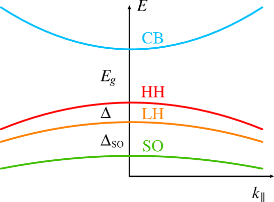
Figure 2: Band structure of a III-V semiconductor quantum well with the $[001]$-growth direction, where $E_{g}$ is the band gap, $\Delta$ is the splitting between the light- and heavy-hole subbands due to quantum-well confinement, and $\Delta_{\mathrm{SO}}$ is the splitting of the valence band due to spin-orbit interaction.

We consider a $[001]$-grown two-dimensional system. In the case of an asymmetric quantum well, due to structure inversion asymmetry along the growth direction, there is an additional spin-orbit term, the Bychkov-Rashba spin-orbit term, which, in the two-band model is given by [42] $\alpha_{R}\mathbf{P\times E\cdot J}$, where $\alpha_{R}$ is the Bychkov-Rashba spin-orbit coupling constant and $\mathbf{E}$ is an effective electric field along the growth direction. Due to confinement along the growth direction, the valence band splits into a heavy-hole subband with $J_{z}=\pm 3/2$ and a light-hole subband with $J_{z}=\pm 1/2$ (see Fig. 2 and Ref. 40). If the splitting $\Delta$ of heavy-hole and light-hole subbands is large, we describe the properties of heavy-holes and light-holes separately, using only the $2\times 2$ submatrices for the $J_{z}=\pm 3/2$ and $J_{z}=\pm 1/2$ states, respectively. The heavy-hole submatrices have the property that $\tilde{J}_{x}=\tilde{J}_{y}=0$ and $\tilde{J}_{z}=\frac{3}{2}\sigma_{z}$. For such a system and low temperatures, only the lowest heavy-hole subband is significantly occupied. In this case, we consider heavy holes only. In the framework of perturbation theory [39], using Eq. (15) and taking into account the Zeeman energy and the Bychkov-Rashba spin-orbit coupling term, the effective Hamiltonian for heavy holes of a quantum dot with lateral confinement potential $U(x,y)$ is given by

$$H=\frac{1}{2m}(P_{x}^{2}+P_{y}^{2})+U(x,y)+H_{\mathrm{SO}}^{\mathrm{HH}}-\frac{1}{2}g_{\perp}\mu_{B}B_{\perp}\sigma_{z},$$ (16)

where $m$ is the effective heavy-hole mass, $\mathbf{P}=\mathbf{p}+|e|\mathbf{A(r)}/c$, $\mathbf{A(r)}=(-yB_{\perp}/2,xB_{\perp}/2,yB_{x}-xB_{y})$, $g_{\perp}$ is the component of the $g$-factor tensor along the growth direction, and

$$H_{\mathrm{SO}}^{\mathrm{HH}}=i\alpha P_{-}^{3}\sigma_{+}+\beta P_{-}P_{+}P_{-}\sigma_{+}+\gamma B_{-}P_{-}^{2}\sigma_{+}+\mathrm{H.c.}$$ (17)

is the spin-orbit coupling of heavy holes consisting of three contributions: the Dresselhaus term ($\beta$) [40], the Rashba term ($\alpha$) [43], and the last term ($\gamma$) combines two effects: orbital coupling via non-diagonal elements in the Luttinger-Kohn Hamiltonian ($\propto P_{\pm}^{2}$) and magnetic coupling via non-diagonal elements in the Zeeman term ($\propto B_{\pm}$). This latter term represents a new type of spin-orbit interaction which is unique for heavy holes [44]. Here, $\alpha=3\gamma_{0}\alpha_{R}\langle E_{z}\rangle/2m_{0}\Delta$, $\beta=-3\gamma_{0}\eta\langle P_{z}^{2}\rangle/2m_{0}\Delta$, $\gamma=3\gamma_{0}\kappa\mu_{B}/m_{0}\Delta$, $\sigma_{\pm}=(\sigma_{x}\pm i\sigma_{y})/2$, $P_{\pm}=P_{x}\pm iP_{y}$, $B_{\pm}=B_{x}\pm iB_{y}$, $m_{0}$ is the free electron mass, $\gamma_{0}$ is the Luttinger parameter [41], $\langle E_{z}\rangle$ is the averaged effective electric field along the growth direction of a quantum dot, and $\Delta$ is the splitting of light-hole and heavy-hole subbands. The splitting between heavy-hole and light-hole subbands $\Delta\sim h^{-2}$, where $h$ is the quantum-dot height.

The spectrum of (16) for parabolic lateral confinement $[U(x,y)=m\omega_{0}^{2}(x^{2}+y^{2})/2]$ and for vanishing spin-orbit interaction ($H_{\mathrm{SO}}^{\mathrm{HH}}=0$) is the Fock-Darwin spectrum split by the Zeeman term [45, 46]. From Eq. (17), it can be seen that $H_{\mathrm{SO}}^{\mathrm{HH}}$ leads to coupling of the two lowest states $|0,\pm 3/2\rangle$ to the states with the opposite spin orientations and different orbital momenta $|l,\mp 3/2\rangle$. Note that the three spin-orbit terms in Eq. (17) differ by symmetry in momentum space and hence mix different states resulting in avoided crossings of the energy levels (see inset of Fig. 3). Due to this spin-orbit mixing of the heavy-hole states, the transitions between the states $|0,\pm 3/2\rangle$ with emission or absorption of an acoustic phonon become possible and this is the main source of spin relaxation and decoherence for heavy-holes [40].

We consider a single-particle quantum dot, in which a heavy hole can occupy one of the low-lying levels. In the following, we study the relaxation of an $n$-level system, the first $n-1$ levels have the same spin and the $n$-th level has the opposite spin orientation. In the framework of Bloch-Redfield theory [47], the Bloch equations for heavy-hole spin motion for such a system in the interaction representation are given by

$$\langle\dot{S}_{z}\rangle = \left(S_{T}-\langle S_{z}\rangle\right)/T_{1}-R(t),$$ (18)

$$\langle\dot{S}_{x}\rangle = -\langle S_{x}\rangle/T_{2},\ \langle\dot{S}_{y}\rangle=-\langle S_{y}\rangle/T_{2},$$ (19)

where $R(t)=W_{n1}\rho_{nn}(t)+\sum_{i=1}^{n-1}W_{ni}\rho_{ii}(t)$, $\rho(t)$ is the density matrix, $W_{ij}$ is the transition rate from state $j$ to state $i$, $S_{T}$ is a constant (which has the value of $\langle S_{z}\rangle$ in thermodynamic equilibrium if $R(t)=0$),

$$\frac{1}{T_{1}}=W_{n1}+\sum_{i=1}^{n-1}W_{in},\ \ \frac{1}{T_{2}}=\frac{1}{2T_{1}}+\frac{1}{2}\sum_{i=2}^{n-1}W_{i1},$$ (20)

where pure dephasing (due to fluctuations along $z$ direction) is absent in the spin decoherence time $T_{2}$ since the spectral function is superohmic. As can be seen from Eq. (18), the spin motion has a complex dependence on the density matrix and, in the general case, there are $n-1$ spin relaxation rates. However, in the case of low temperatures ($\hbar qs_{\alpha}\gg k_{\mathrm{B}}T$), when phonon absorption becomes strongly suppressed, solving the master equation, we find that $R(t)\approx 0$. Therefore, there is only one spin relaxation time $T_{1}$. In this limit, the last sum in Eq. (20) is negligible and the spin decoherence time saturates, i.e., $T_{2}=2T_{1}$.

Note that in contrast to electrons [48] there are no interference effects between different spin-orbit coupling terms, thus the total spin relaxation rate $1/T_{1}$ is the sum of rates $1/T_{1}=1/T_{1}^{\mathrm{D}}+1/T_{1}^{\mathrm{BR}}+1/T_{1}^{\parallel}$ [40, 44]:

$$\frac{1}{T_{1}^{\mathrm{BR}}} \propto \alpha^{2}\omega_{Z}^{7}\left(\frac{\omega_{+}^{3}}{3\omega_{+}+\omega_{Z}}-\frac{\omega_{-}^{3}}{3\omega_{-}-\omega_{Z}}\right)^{2},$$

$$\frac{1}{T_{1}^{\mathrm{D}}} \propto \beta^{2}\omega_{Z}^{3}\left(\frac{\omega_{+}}{\omega_{+}+\omega_{Z}}-\frac{\omega_{-}}{\omega_{-}-\omega_{Z}}\right)^{2},$$

$$\frac{1}{T_{1}^{\parallel}} \propto \gamma^{2}B_{\parallel}^{2}\omega_{\mathrm{Z}}^{5}\left(\frac{\omega_{+}^{2}}{2\omega_{+}+\omega_{Z}}+\frac{\omega_{-}^{2}}{2\omega_{-}-\omega_{Z}}\right)^{2},$$ (21)

where $\omega_{\pm}=\sqrt{\omega_{0}^{2}+\omega_{c}^{2}/4}\pm\omega_{c}/2$, $\omega_{\mathrm{Z}}=g_{\perp}\mu_{B}B_{\perp}/\hbar$, $B_{\parallel}=\sqrt{B_{x}^{2}+B_{y}^{2}}$.

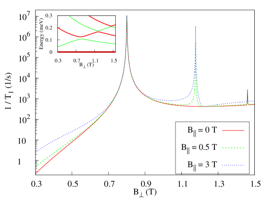
Figure 3: Heavy hole spin relaxation rate $1/T_{1}$ in a GaAs quantum dot versus an applied perpendicular magnetic field $B_{\perp}$ (the height of the quantum dot is chosen to be $h=5\>$nm, the lateral size $l_{0}=\sqrt{\hbar/m\omega_{0}}=40\>$nm, $\kappa=1.2$, $\gamma_{0}=2.5$, $g_{\perp}=2.5$ [49], and the other parameters are given in Ref. [40]). Inset: Energy differences of lowest excited levels with respect to the ground state $E_{0,+3/2}$. The second avoided crossing comes from the spin-orbit interaction and the in-plane magnetic field $B_{\parallel}$ (3rd term in Eq. 17). The anticrossing gap is proportional to $B_{\parallel}$, implying that the coupling between corresponding states can be controlled externally.

In Fig. 3 the total spin relaxation rate $1/T_{1}$ is plotted as a function of perpendicular magnetic field $B_{\perp}$. There are three peaks in the relaxation rate curve at $\omega_{\mathrm{Z}}=\omega_{-},\ 2\omega_{-}$, and $3\omega_{-}$, which are caused by strong spin mixing at the anticrossing points. In the inset, the first (third) avoided crossing resulting from Dresselhaus (Rashba) spin-orbit coupling corresponds to the first (third) peak of the spin relaxation curve in Fig. 3. At non-zero in-plane magnetic fields ($B_{\parallel}$), there is an additional peak which is due to an anticrossing between the energy levels $E_{0,+3/2}$ and $E_{2,-3/2}$ (see the second avoided crossing in the inset). Note that the spin relaxation rate for heavy holes is comparable to that for electrons [40, 50] due to the fact that spin-orbit coupling of heavy holes is strongly suppressed for flat quantum dots (see Eq. (17)), as confirmed by a recent experiment [51].

7 Electric dipole spin resonance for heavy holes

Let us now consider methods for the manipulation and detection of the heavy-hole spin in quantum dots. For electrons in two-dimensional structures, an applied oscillating in-plane magnetic field couples spin-up and spin-down states via magnetic-dipole transitions and is commonly used in electron spin resonance, Rabi oscillation, and spin echo experiments [10]. It can be shown that magnetic-dipole transitions ($\Delta n=0$, $\Delta\ell=0$, and $\Delta s=\pm 1$) are forbidden and, due to spin-orbit mixing of the states $|0,\pm 3/2\rangle$ with $i\beta_{1}^{\pm}|1,\mp 3/2\rangle$, electric-dipole transitions ($\Delta n=\pm 1$, $\Delta\ell=\pm 1$, and $\Delta s=0$) are most likely to occur. Therefore, the heavy holes are affected by the oscillating electric field component and not by the magnetic one.

We consider a circularly polarized electric field rotating in the XY-plane with frequency $\omega$: $\mathbf{E}(t)=E(\sin\omega t,-\cos\omega t,0)$. Therefore, the interaction of heavy holes with the electric field is described by the Hamiltonian $H^{E}(t)=(|e|E/m\omega)(\cos\omega tP_{x}+\sin\omega tP_{y})$. The coupling between the states $|\pm\rangle$ is given by $\langle+|H^{E}(t)|-\rangle=H^{E}_{+-}=\left(H^{E}_{-+}\right)^{*}=d_{\mathrm{SO}}Ee^{-i\omega t}$, where

$$d_{\mathrm{SO}}=(|e|l/2\omega)(\beta_{1}^{-}\omega_{-}+\beta_{1}^{+}\omega_{+})$$ (22)

is an effective dipole moment of a heavy hole depending on Dresselhaus spin-orbit coupling constants, perpendicular magnetic field $B_{\perp}$, lateral size of a quantum dot, and frequency $\omega$ of an rf electric field.

In the framework of the Bloch-Redfield theory [47] (taking into account also off-diagonal matrix elements), the effective master equation for the density matrix $\rho_{nm}$ assumes the form of Bloch equations [47], with the detuning of the rf field given by $\delta_{\mathrm{rf}}=\omega_{\mathrm{Z}}-\omega$. $2d_{\mathrm{SO}}E/\hbar$ is the Larmor frequency, $T_{1}=1/(W_{+-}+W_{-+})$ the spin relaxation time ($W_{nm}$ is the transition rate from state $m$ to state $n$), $T_{2}=2T_{1}$ [40] the spin decoherence time, and $\rho_{z}^{T}=(W_{+-}-W_{-+})T_{1}$ the equilibrium value of $\rho_{z}$ without rf field.

The coupling energy between a heavy hole and an oscillating electric field is given by

$$\langle H^{E}(t)\rangle=\mathrm{Tr}(\rho H^{E}(t))=-\mathbf{d}_{\mathrm{SO}}\cdot\mathbf{E}(t),$$ (23)

where $\mathbf{d}_{\mathrm{SO}}=d_{\mathrm{SO}}(i\rho_{-+}-i\rho_{+-},\rho_{+-}+\rho_{-+},0)$ is the dipole moment of a heavy hole. Therefore, the rf power $P=-d\langle H^{E}(t)\rangle/dt=-\omega d_{\mathrm{SO}}E\rho_{-}$ absorbed by a heavy-hole spin system in the stationary state is given by [52]

$$P=\frac{2\omega(d_{\mathrm{SO}}E)^{2}T_{2}\rho_{z}^{T}/\hbar}{1+\delta_{\mathrm{rf}}^{2}T_{2}^{2}+(2d_{\mathrm{SO}}E/\hbar)^{2}T_{1}T_{2}}.$$ (24)

In Fig. 4, the dependence of $P$ on a perpendicular magnetic field $B_{\perp}$ and frequency $\omega$ of the oscillating electric field is plotted. The rf power $P$ absorbed by the system has three resonances and one resonant dip. The first resonance appears when the energy of rf radiation equals the Zeeman energy of heavy holes: $B_{\perp}^{\mathrm{r},1}=\hbar\omega/g_{\perp}\mu_{\mathrm{B}}$. The shape of this resonance (at certain $\omega$) is given by $P\approx\hbar\omega\rho_{z}^{T}/2\hbar[1+\hbar^{2}\delta_{\mathrm{rf}}^{2}T_{2}/(2d_{\mathrm{SO}}E)^{2}T_{1}]$.

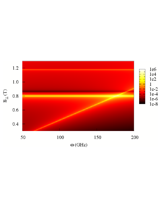
Figure 4: Absorbed power $P\>$(meV$/$s) as a function of perpendicular magnetic field $B_{\perp}$ and rf frequency $\omega$ ($T_{2}=2T_{1}$, $E=2.5\>$V$/$cm, $B_{\parallel}=1\>$T, and the other parameters are the same as those in Fig. 3).

If the first and second resonances are well separated ($\omega\ll\omega_{-}$), then the absorbed power can be estimated as

$$P\approx 2\omega(d_{\mathrm{SO}}E)^{2}\rho_{z}^{T}/\hbar\delta_{\mathrm{rf}}^{2}T_{2}$$ (25)

in the region of the second and third resonances and the resonant dip. The second resonance corresponds to an anticrossing of the levels $E_{0,-3/2}$ and $E_{1,3/2}$ (see the first avoided crossing in the inset of Fig. 3) at $\omega_{-}=\omega_{\mathrm{Z}}$ [40] (at $B=B_{\perp}^{\mathrm{r},2}$). At the anticrossing point, there is strong mixing of the spin-up and spin-down states and the dipole moment of a heavy-hole spin system is maximal $d_{\mathrm{SO}}^{\mathrm{max}}=|e|l\omega_{\mathrm{Z}}/2\omega$ and equals half of the lowest electric dipole moment of a quantum dot ($|e|l\omega_{-}/\omega$). Therefore, the height of the second resonance is given by $(el\omega_{\mathrm{Z}}E)^{2}/2\hbar\omega\delta_{\mathrm{rf}}^{2}T_{2}$. The resonant dip appears at $B_{\perp}^{\mathrm{d}}=(\hbar\omega_{0}/2g_{\perp}\mu_{\mathrm{B}})\sqrt{2m_{0}/g_{\perp}m}$, which corresponds to $\beta_{1}^{-}\omega_{-}+\beta_{1}^{+}\omega_{+}=0$ and to zero dipole moment (see Eq. (22)). The third resonance reflects the peak in the spin decoherence rate $T_{2}^{-1}$ due to an applied in-plane magnetic field (see Fig. 3) at the second anticrossing point (the second avoided crossing in inset of Fig. 3) at $2\omega_{-}=\omega_{\mathrm{Z}}$ ($B_{\perp}^{\mathrm{r},3}=4\hbar\omega_{0}/g_{\perp}\mu_{\mathrm{B}}\sqrt{1+4m_{0}/g_{\perp}m}$). From the positions of the resonances we can determine $g_{\perp}$, $m$, and $\omega_{0}$, from the shape and the height of those we can extract information about the spin-orbit interaction constants $\alpha$, $\beta$, and spin-orbit interaction strength due to in-plane magnetic field (which is proportional to $\gamma_{0}\kappa/\Delta$). Moreover, we can determine the dependence of the spin relaxation and decoherence times on $B_{\perp}$.

8 Conclusions

We have discussed the rich dynamics of single electron spins in single and double quantum dots due to hyperfine interaction with the nuclei. Key features are non-exponential decays of various kinds and a remarkable universal phase-shift. Further, we have studied spin decoherence and relaxation of heavy holes in quantum dots due to spin-orbit coupling. The spin relaxation time $T_{1}$ for heavy holes in flat quantum dots can be comparable to that for electrons [40, 50] as confirmed by experiment [51]. The spin decoherence time for heavy holes is given by $T_{2}=2T_{1}$ at low temperatures. There is strong spin mixing at energy-level crossings resulting in a non-monotonic dependence $T_{1}(B)$. We have proposed a new method for manipulation of a heavy-hole spin in a quantum dot via rf electric fields. This method can be used for detection of heavy-hole spin resonance signals, for spin manipulation, and for determining important parameters of heavy holes [44].

Aknowledgments: We aknowledge financial support from the Swiss NSF, the NCCR Nanoscience and JST ICORP.

References

- 1. D. Loss and D. P. DiVincenzo, Quantum computation with quantum dots, Phys. Rev. A. 57, 120–126, (1998).
- 2. S. Tarucha, D. G. Austing, T. Honda, R. J. van der Hage, and L. P. Kouwenhoven, Shell filling and spin effects in a few electron quantum dot, Phys. Rev. Lett. 77(17), 3613–3616, (1996).
- 3. M. Ciorga, A. S. Sachrajda, P. Hawrylak, C. Gould, P. Zawadzki, S. Jullian, Y. Feng, and Z. Wasilewski, Addition spectrum of a lateral dot from coulomb and spin-blockade spectroscopy, Phys. Rev. B. 61(24), R16315–R16318, (2000).
- 4. J. M. Elzerman, R. Hanson, J. S. Greidanus, L. H. Willems van Beveren, S. De Franceschi, L. M. K. Vandersypen, S. Tarucha, and L. P. Kouwenhoven, Few-electron quantum dot circuit with integrated charge read out, Phys. Rev. B. 67(16), 161308, (2003).
- 5. T. Hayashi, T. Fujisawa, H. D. Cheong, Y. H. Jeong, and Y. Hirayama, Coherent manipulation of electronic states in a double quantum dot, Phys. Rev. Lett. 91(22), 226804, (2003).
- 6. J. R. Petta, A. C. Johnson, C. M. Marcus, M. P. Hanson, and A. C. Gossard, Manipulation of a single charge in a double quantum dot, Phys. Rev. Lett. 93(18), 186802, (2004).
- 7. J. M. Elzerman, R. Hanson, L. H. Willems van Beveren, B. Witkamp, L. M. K. Vandersypen, and L. P. Kouwenhoven, Single-shot read-out of an individual electron spin in a quantum dot, Nature. 430, 431–435, (2004).
- 8. R. Hanson, L. H. van Beveren, I. T. Vink, J. M. Elzerman, W. J. Naber, F. H. Koppens, L. P. Kouwenhoven, and L. M. Vandersypen, Single-shot readout of electron spin states in a quantum dot using spin-dependent tunnel rates, Phys. Rev. Lett. 94(19), 196802, (2005).
- 9. J. R. Petta, A. C. Johnson, J. M. Taylor, E. A. Laird, A. Yacoby, M. D. Lukin, C. M. Marcus, M. P. Hanson, and A. C. Gossard, Coherent manipulation of coupled electron spins in semiconductor quantum dots, Science. 309(5744), 2180–2184, (2005).
- 10. F. H. L. Koppens, C. Buizert, K. J. Tielrooij, I. T. Vink, K. C. Nowack, T. Meunier, L. P. Kouwenhoven, and L. M. K. Vandersypen, Driven coherent oscillations of a single electron spin in a quantum dot, Nature. 442, 766–771, (2006).
- 11. V. Cerletti, W. A. Coish, O. Gywat, and D. Loss, TUTORIAL: Recipes for spin-based quantum computing, Nanotechnology. 16, 27, (2005).
- 12. W. A. Coish and D. Loss, Quantum computing with spins in solids, http://arXiv.org/cond-mat/0606550. (2006).
- 13. D. Paget, G. Lampel, B. Sapoval, and V. I. Safarov, Low field electron-nuclear spin coupling in gallium arsenide under optical pumping conditions, Phys. Rev. B. 15, 5780–5796, (1977).
- 14. J. Schliemann, A. Khaetskii, and D. Loss, TOPICAL REVIEW: Electron spin dynamics in quantum dots and related nanostructures due to hyperfine interaction with nuclei, J. Phys.: Condens. Matter. 15, 1809 (Dec., 2003).
- 15. J. M. Taylor, J. R. Petta, A. C. Johnson, A. Yacoby, C. M. Marcus, and M. D. Lukin, Relaxation, dephasing, and quantum control of electron spins in double quantum dots, http://arXiv.org/cond-mat/0602470. (2006).
- 16. G. Burkard, D. Loss, and D. P. DiVincenzo, Coupled quantum dots as quantum gates, Phys. Rev. B. 59, 2070–2078, (1999).
- 17. A. V. Khaetskii, D. Loss, and L. Glazman, Electron spin decoherence in quantum dots due to interaction with nuclei, Phys. Rev. Lett. 88(18), 186802, (2002).
- 18. I. A. Merkulov, A. L. Efros, and M. Rosen, Electron spin relaxation by nuclei in semiconductor quantum dots, Phys. Rev. B. 65(20), 205309, (2002).
- 19. W. A. Coish and D. Loss, Hyperfine interaction in a quantum dot: Non-Markovian electron spin dynamics, Phys. Rev. B. 70(19), 195340, (2004).
- 20. D. Stepanenko, G. Burkard, G. Giedke, and A. Imamoǧlu, Enhancement of electron spin coherence by optical preparation of nuclear spins, Phys. Rev. Lett. 96(13), 136401, (2006).
- 21. D. Klauser, W. A. Coish, and D. Loss, Nuclear spin state narrowing via gate–controlled Rabi oscillations in a double quantum dot, Phys. Rev. B. 74(20), 205302, (2006).
- 22. G. Giedke, J. M. Taylor, D. D’Alessandro, M. D. Lukin, and A. Imamoğlu, Quantum measurement of a mesoscopic spin ensemble, Phys. Rev. A. 74(3), 032316, (2006).
- 23. F. H. L. Koppens, J. A. Folk, J. M. Elzerman, R. Hanson, L. H. W. van Beveren, I. T. Vink, H. P. Tranitz, W. Wegscheider, L. P. Kouwenhoven, and L. M. K. Vandersypen, Control and detection of singlet-triplet mixing in a random nuclear field, Science. 309, 1346–1350, (2005).
- 24. P. Maletinsky, A. Badolato, and A. Imamoǧlu, Dynamics of quantum dot nuclear spin polarization controlled by a single electron, http://arXiv.org/abs/0704.3684v1. (2007).
- 25. J. Baugh, Y. Kitamura, K. Ono, and S. Tarucha, Large nuclear Overhauser fields detected in vertically-coupled double quantum dots, http://arxiv.org/abs/0705.1104. (2007).
- 26. D. Reilly, C. M. Marcus, et al. Unpublished.
- 27. P. Maletinsky, C. W. Lai, A. Badolato, and A. Imamoǧlu, Nonlinear dynamics of quantum dot nuclear spins, Phys. Rev. B. 75, 035409, (2007).
- 28. K. Ono, D. G. Austing, Y. Tokura, and S. Tarucha, Current rectification by pauli exclusion in a weakly coupled double quantum dot system, Science. 297, 1313–1317, (2002).
- 29. K. Ono and S. Tarucha, Nuclear-spin-induced oscillatory current in spin-blockaded quantum dots, Phys. Rev. Lett. 92(25), 256803, (2004).
- 30. F. H. L. Koppens, D. Klauser, W. A. Coish, K. C. Nowack, L. P. Kouwenhoven, D. Loss, and L. M. K. Vandersypen, Universal phase shift and non-exponential decay of driven single-spin oscillations, http://arXiv.org/cond-mat/0703640. (2007).
- 31. W. Yao, R.-B. Liu, and L. J. Sham, Theory of electron spin decoherence by interacting nuclear spins in a quantum dot, Phys. Rev. B. 74(19), 195301, (2006).
- 32. N. Shenvi, R. de Sousa, and K. B. Whaley, Nonperturbative bounds on electron spin coherence times induced by hyperfine interactions, Phys. Rev. B. 71(14), 144419, (2005).
- 33. C. Deng and X. Hu, Analytical solution of electron spin decoherence through hyperfine interaction in a quantum dot, Phys. Rev. B. 73(24), 241303, (2006). Erratum: Phys. Rev. B 74, 129902.
- 34. W. A. Coish and D. Loss, Singlet-triplet decoherence due to nuclear spins in a double quantum dot, Phys. Rev. B. 72(12), 125337, (2005).
- 35. E. A. Laird, J. R. Petta, A. C. Johnson, C. M. Marcus, A. Yacoby, M. P. Hanson, and A. C. Gossard, Effect of exchange interaction on spin dephasing in a double quantum dot, Phys. Rev. Lett. 97(5), 056801, (2006).
- 36. A. Peres, Quantum Theory: Concepts and Methods. (Kluwer Academic Publishers, 1993).
- 37. D. Klauser, W. A. Coish, and D. Loss, Quantum-dot spin qubit and hyperfine interaction, http://arXiv.org/cond-mat/0604252. (2006).
- 38. J. M. Luttinger and W. Kohn, Motion of electrons and holes in perturbed periodic fields, Phys. Rev. 97(4), 869–883, (1955).
- 39. B. P. Zakharchenya and F. Mier, Eds., Optical Orientation. (North-Holland, Amsterdam, 1984).
- 40. D. V. Bulaev and D. Loss, Spin relaxation and decoherence of holes in quantum dots, Phys. Rev. Lett. 95, 076805, (2005).
- 41. J. M. Luttinger, Quantum theory of cyclotron resonance in semiconductors: General theory, Phys. Rev. 102, 1030, (1956).
- 42. R. Winkler, Rashba spin splitting in two-dimensional electron and hole systems, Phys. Rev. B. 62, 4245, (2000).
- 43. R. Winkler, H. Noh, E. Tutuc, and M. Shayegan, Anomalous Rashba spin splitting in two-dimensional hole systems, Phys. Rev. B. 65, 155303, (2002).
- 44. D. V. Bulaev and D. Loss, Electric dipole spin resonance for heavy holes in quantum dots, Phys. Rev. Lett. 98, 097202, (2007).
- 45. V. Fock, Bemerkung zur Quantelung des harmonischen Oszillators im Magnetfeld, Z. Phys. 47, 446–448, (1928).
- 46. C. G. Darwin, The diamagnetism of the free electron, Proc. Cambridge Philos. Soc. 27, 86–90, (1930).
- 47. K. Blum, Density Matrix Theory and Applications. (Plenum, New York, 1996).
- 48. V. N. Golovach, A. Khaetskii, and D. Loss, Phonon-Induced Decay of the Electron Spin in Quantum Dots, Phys. Rev. Lett. 93, 016601, (2004).
- 49. H. W. van Kestern, E. C. Cosman, W. A. J. A. van der Poel, and C. T. Foxton, Fine structure of excitons in type-II GaAs/AlAs quantum wells, Phys. Rev. B. 41, 5283, (1990).
- 50. D. V. Bulaev and D. Loss, Spin relaxation and anticrossing in quantum dots: Rashba versus Dresselhaus spin-orbit coupling, Phys. Rev. B. 71, 205324, (2005).
- 51. D. Heiss, S. Schaeck, H. Huebl, M. Bichler, G. Abstreiter, J. J. Finley, D. V. Bulaev, and D. Loss, Observation of extremely slow hole spin relaxation in self-assembled quantum dots, http://arxiv.org/abs/0705.1466. (2007).
- 52. A. Abragam, The Principles of Nuclear Magnetism. (Oxford University Press, London, 1961).