X-ray Luminosity Functions of Normal Galaxies in the GOODS

Abstract

We present soft (0.5-2 keV) X-ray luminosity functions (XLFs) in the Great Observatories Origins Deep Survey (GOODS) fields, derived for galaxies at $z\sim 0.25$ and 0.75. SED fitting was used to estimate photometric redshifts and separate galaxy types, resulting in a sample of 40 early-type galaxies and 46 late-type galaxies. We estimate k-corrections for both the X-ray/optical and X-ray/NIR flux ratios, which facilitates the separation of AGN from the normal/starburst galaxies. We fit the XLFs with a power-law model using both traditional and Markov-Chain Monte Carlo (MCMC) procedures. A key advantage of the MCMC approach is that it explicitly takes into account upper-limits and allows errors on “derived” quantities such as luminosity densities to be computed directly (i.e., without potentially questionable assumptions concerning the propagation of errors). The slopes of the early-type galaxy XLFs tend to be slightly flatter than the late-type galaxy XLFs although the effect is significant at only the 90% and 97% levels for z$\sim 0.25$ and 0.75. The XLFs differ between $z<0.5$ and $z>0.5$, at $>99\%$ significance levels for early-type, late-type and all (early and late-type) galaxies. We also fit Schechter and log-normal models to the XLFs, fitting the low and high redshift XLFs for a given sample simultaneously assuming only pure luminosity evolution. In the case of log-normal fits, the results of MCMC fitting of the local FIR luminosity function were used as priors for the faint and bright-end slopes (similar to “fixing” these parameters at the FIR values except here the FIR uncertainty is included). The best-fit values of the change in $\log L^{*}$ with redshift were $\Delta\log L^{*}=0.23\pm 0.16$ dex (for early-type galaxies) and $0.34\pm 0.12$ dex (for late-type galaxies), corresponding to $(1+z)^{1.6}$ and $(1+z)^{2.3}$. These results were insensitive to whether the Schechter or log-normal function was adopted.

1. Introduction

Recently (Norman et al., 2004, hereafter N04) presented the first X-ray luminosity functions (XLFs) of normal/starburst galaxies at cosmologically-interesting redshifts (at z $\sim$ 0.3 and 0.7). These XLFs were derived from the Chandra Deep Field North (2 Ms) and South (1 Ms) surveys (hereafter the “CDF” fields). It was found that the normal galaxy XLF was consistent in normalization and shape to the far-infrared LF, assuming pure luminosity evolution of $\sim(1+z)^{3}$. While the errors were large due to the limited numbers of galaxies in each luminosity bin, the estimated star-formation rate (SFR) derived from the XLFs was found to be consistent with other SFR measures such as the H$\alpha$ luminosity. As discussed in N04, an interesting aspect of the XLF is that the X-ray emission from star-forming galaxies often has a large component due to X-ray binaries, particularly at hard X-ray energies above 2 keV. Therefore, the XLF is in part a probe of the binary stellar mass functions, and hence indirectly a measure of the SFR. It is quite possible that binaries play a critical role in the evolution of the majority of stellar systems, and X-ray emission provides one of very few direct probes of such phenomena.

The Great Observatories Origins Deep Survey (GOODS; Giavalisco et al., 2003) is a multi-wavelength survey of a sub-area of the CDF fields. This survey entails deep imaging by three of NASA’s Great Observatories: the Hubble Space Telescope, the Chandra X-ray Observatory, and the Spitzer Space Telescope, as well as extensive photometric and spectroscopic observation by ground based facilities. These data allow the extension of the N04 results in several new directions. First, improved redshift determinations are now available for many of the sources. Second, the multi-band data have been used to model the spectral-energy distributions (SEDs) of the sources and estimate their spectral types. Therefore XLFs can now be generated as a function of galaxy spectral type, which is the primary goal of this paper. Finally, we have improved the selection of AGN vs. normal/starburst galaxies over N04 by applying k-corrections to both X-ray/optical and X-ray/NIR flux ratios. Such k-corrections are critical to correctly separating AGN from normal galaxies (Bauer et al., 2004).

A motivation for deriving galaxy type-selected XLFs is the fact that there are multiple contributors to the X-ray emission of galaxies, namely low-mass X-ray binaries (LMXRB), high-mass X-ray binaries (HMXRB), hot ISM, AGN, and to a lesser extent, individual supernovae (SN) and massive stars, with the relative contribution of these expected to be dependent on galaxy type (see Ptak, 2001, for a review). Specifically, the X-ray emission of early-type galaxies is known to be dominated by LMXRB emission, and in the case of massive, gas-rich ellipticals, hot ISM (at the virial temperature of the galaxy). Late-type spiral galaxies should have significant contributions from both LMXRB and HMXRB populations, with the former being associated with the older (t $\gtrsim 10^{8-9}$ year) populations. Late-type spiral galaxies often exhibit hot ISM due to heating associated with recent episodes of star formation. Finally, starburst galaxies should have the largest contribution from hot ISM (including potentially a superwind outflow) and HMXRB (see Persic & Rephaeli, 2003). We would therefore naively expect somewhat different evolution in the X-ray luminosity density of these various galaxy types, with the LMXRB contribution following the global SFR history of the Universe with a delay of the order of the evolutionary time scale of low-mass stars, i.e., $\sim 10^{9}$ years (Ghosh & White, 2001) and the HMXRB and hot ISM contribution tracking the SFR history instantaneously (relative to a Hubble time).

In this paper we are primarily concerned with sources with $L_{X}<10^{42}$ erg s^-1, and hence any AGN present would be a low-luminosity AGN (LLAGN). LLAGN are found in all galaxy types, with LINERs preferentially being found in early-type galaxies (see Ho et al., 2003, and references therein). As in N04, we assess the impact of AGN by classifying sources based on a Bayesian statistical analysis. In the Appendix we also separately address the properties of the X-ray flux ratios (i.e., ratio of X-ray to optical and near-IR flux) which provide important criteria for source classification. Ascertaining the presence of any luminosity or redshift dependence in the X-ray/optical or X-ray/NIR flux ratios would also indicate possible evolution of the relative contributions of different sources of X-ray flux in galaxies, i.e., LMXRB, HMXRB, hot gas, and AGN (for examples of study of the evolution of X-ray/optical flux ratios, please see Ptak et al., 2001; Hornschemeier et al., 2002).

This paper is organized as follows. In Section 2 we describe our sample selection and data analysis. The results of our analysis are given in Section 3, and we discuss the results in Section 4. In the Appendix we give the details of our galaxy/AGN source classification procedure, basic statistics concerning the sample, and a discussion of the X-ray/optical and X-ray/NIR flux ratios. We assume the WMAP cosmology of $H_{0}$ = 70 km s^-1 Mpc^-1, $\Omega_{m}=0.3$ and $\Omega_{\Lambda}=0.7$.

2. Methodology

2.1. X-ray Sample Selection and Redshifts

The X-ray data used in our analysis are taken from Alexander et al. (2003), where the positions and X-ray fluxes for sources in both the CDF-N and CDF-S are tabulated. Bauer et al. (2007) have carried out detailed matching of the GOODS ACS data with the Alexander et al. (2003) X-ray catalog, assigning matching probabilities based on optical faintness of potential counterparts, resulting in 263 (185) sources in the CDF-N (CDF-S) having a single ACS counterpart. We found 44 (28) CDF-N (CDF-S) sources with no optical counterpart, while 3 (4) with multiple counterparts were not included in our analysis. We also included the off-nuclear X-ray sources (14 in the CDF-N and 6 in the CDF-S; e.g., Hornschemeier et al., 2004). We then used the ACS coordinates in the Bauer catalog to match with the publicly available GOODS spectroscopic redshift catalogs and Mobasher et al. (2004) photometric redshift catalog to obtain both redshifts and spectral types for all sources. Stars were excluded. The main parameters for each galaxy are the soft-band (0.5-2.0 keV) flux (from Alexander et al., 2003), the hardness ratio (defined as $\frac{H-S}{H+S}$ where H is the 2-8 keV vignetting-corrected count rate and S is the 0.5-2.0 keV vignetting-corrected count rate; from Alexander et al. 2003), the redshifts, and the optical spectral types. We broadly divided the spectral types into the groups early-type, late-type, and starburst/irregular galaxies, however we only extract XLFs for early-type and late-type galaxies since the numbers of irregular galaxies were very small.

2.1.1 Photometric Redshifts

The photometric redshifts for GOODS fields are estimated using template fitting technique (Mobasher et al 1996; Chen et al 1999; Arnouts et al., 1999; Benitez 2001; Bolzonella et al 2000, Dahlen et al. 2007). The rest-frame Spectral Energy Distribution (SED) for galaxies of different types are convolved with filter response functions of the filters used in photometric observations of galaxies. The convolved SEDs, shifted in redshift space, were then fitted to observed SEDs of individual galaxies by minimizing the $\chi^{2}$ function

$$\chi^{2}=\Sigma_{i=1}^{n}[(F^{i}_{obs}-\alpha F^{i}_{template})/\sigma^{i})]^{2}$$

where the summation, $i$, is over the passbands (i.e. number of photometric points) and $n$ is the total number of passbands. $F^{i}_{obs}$ and $F^{i}_{template}$ are, respectively, the observed and template fluxes at any given passband. $\sigma^{i}$ is the uncertainty in the observed flux and $\alpha$ is the normalization. The redshift and SED (i.e. spectral type) corresponding to the minimum $\chi^{2}$ value for a given galaxy were then assigned to that galaxy. We used priors based on luminosity functions (LFs). The main effect of a LF prior is to discriminate between cases in which the redshift probability distribution function, which identifies the most likely redshift, shows two or multiple peaks (i.e. more than a single optimum redshift) due to confusion between the Lyman break and the 4000 Å  break features. The absolute magnitudes of the object at the redshift peaks can then discriminate between these possibilities. Absorption due to intergalactic HI is included using the parametrization in Madau (1995).

We use template spectral energy distributions (SEDs) for normal galaxies consisting of E, Sbc, Scd and Im from Colman et al (1980) and two starburst templates from Kinney et al (1996)-(SB2 and SB3). To increase the spectral resolution, we construct intermediate-type templates by using the weighted mean of the adjacent templates and interpolate between them. This is done by defining five intermediate-type templates between the main spectral types used. Therefore, we use a total of 31 SED templates in this study. Photometric redshifts were then measured using the the observed photometry in GOODS-N (UBVRizJK) and GOODS-S (UBVRiJHK).

2.1.2 Spectroscopic Redshifts

For a subset of the galaxies, we use the available spectroscopic redshifts. The majority of the spectroscopic redshifts were derived from Keck DEIMOS data for the CDF-N (see Wirth et al., 2004, and references therein) and VLT FORS2 or VIMOS data for the CDF-S (Szokoly et al., 2004; Vanzella et al., 2006). The limiting magnitude for spectroscopic redshift determination was typically $R_{AB}\sim 24$. If a spectroscopic redshift was not available then a photometric redshift was used, with the photometric redshift limiting magnitude typically being $R_{AB}\sim 25$ (Mobasher et al., 2004). In cases where a quality assessment was available for the spectroscopic redshift and was considered to be poor, and a photometric redshift with error $\delta z<0.2$ was available , the photometric redshift was used. In cases where there was no spectroscopic redshift quality given and a photometric redshift with error $\delta z<0.1$ was available, the photometric redshift was used. This resulted in 204 (129) and 157 (116) total (spectroscopic) redshift determinations for the CDF-N and CDF-S sources, respectively (i.e., 73% and 82% of the GOODS X-ray sources with a unique optical counterpart have a redshift estimate). The redshift distributions are shown in Figure 1.

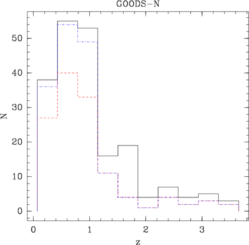
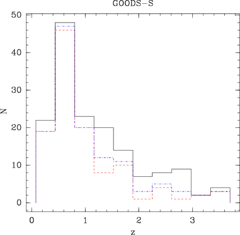
Figure 1.— The redshift distributions for the CDF-N (left) and CDF-S (right) fields. The spectroscopic redshift distributions are shown in blue with dot-dashed lines. In cases where the spectroscopic redshift quality was unknown or flagged as low and the photometric redshift error was small (see text for details), the photometric redshift was adopted. This distribution of sources for which a spectroscopic redshift was adopted is shown in red with dashed lines.

In cases where both a photometric and spectroscopic redshift were available, the mean absolute redshift difference was 0.09 (CDF-N) and 0.13 (CDF-S) after removing a small number of outliers with $\Delta z\equiv|z_{\rm spec}-z_{\rm phot}|>0.5$. In Figure 2 we plot the difference between the photometric and spectroscopic redshift for sources with both measurements. The errors plotted in the figure are based solely on the photometric redshift errors. This figure shows that our typical redshift uncertainty is $\Delta z\sim 0.1-0.2$ for $z\lesssim 1.5$, and increases significantly for $z>1.5$. We conservatively limit our analysis to $z\leq 1.2$. This leaves a total of 148 sources in the CDF-N and 95 sources in the CDF-S regions, of which 138 and 81 have soft-band X-ray detections. Note that 131 (CDF-N) and 75 (CDF-S) of the X-ray sources have $L_{X}<1\times 10^{43}\rm\ ergs\ s^{-1}$, the highest X-ray luminosity considered in the X-ray luminosity functions discussed here.

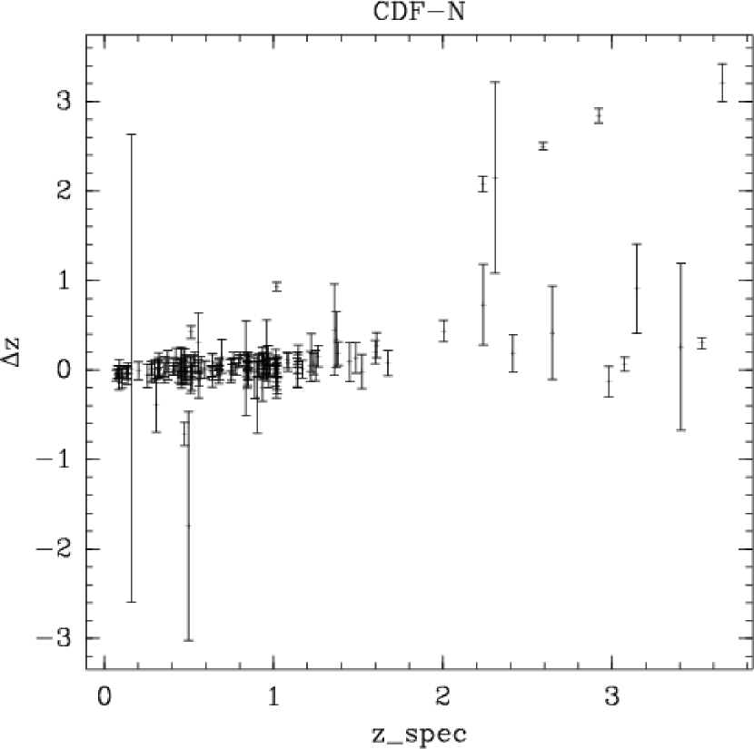
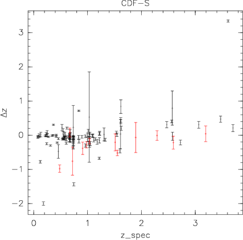
Figure 2.— $\Delta z=z_{spec}-z_{phot}$ plotted as a function of $z_{spec}$ for CDF-N (left) and CDF-S (right). In the CDF-S plot, the sources with poor spectroscopic redshift determinations (often based on a single line identification) are shown in red and marked with crosses) The errors plotted for the points are based solely on the photometric redshift error.

2.2. K-Corrections

The soft-band X-ray fluxes, listed in Alexander et al. (2003), are based on the observed count rates and a count rate to flux conversion computed from an effective photon index (based on band ratios). This photon index ($\Gamma$) was used to “k-correct” the observed fluxes, i.e., $F_{X,kcor}=(1+z)^{\Gamma-2}F_{X,obs}$, and $L_{X}=4\pi d_{L}^{2}F_{X,kcor}$ where $d_{L}$ is the luminosity distance. In Appendix A we present the sources, the adopted redshifts and X-ray luminosities.

For a given band Q, we define $F_{Q}$ to be $\nu F_{\nu}$ at the central frequency of the band $\nu_{Q}$. Since the GOODS magnitudes are in the AB system, $\log(F_{X}/F_{Q})$ is given by $\log F_{X}+0.4(Q+48.6)-\log\nu_{Q}$, e.g., in the case of R band, $\log(F_{X}/F_{R})=\log F_{X}+0.4R_{AB}+4.8$. The optical magnitudes were k-corrected by interpolating between the magnitudes whose central wavelengths bracket $(1+z)\lambda$, where $\lambda$ is the central wavelength of the filter of interest (e.g., 4400Å for B-band). The bandpass correction term (1+z) was also included in the k-correction (Blanton et al., 2003). In Figure 3 we show the k-corrections applied to R and $\rm K_{s}$ band flux ratios. Note that in the case of $\rm K_{s}$ band magnitudes, the interpolation discussed above necessarily amounts to an extrapolation since $\rm K_{s}$ is the longest wavelength band in the dataset and every source considered here has $z>0$. The corrections are plotted separately for each spectral type, where it can be seen that the largest k-corrections occur for B band fluxes from early-type galaxies, which is not surprising considering their red color. Also, as mentioned in Bauer et al. (2004), the k-corrections to the flux ratios are dominated by the optical correction rather than the X-ray correction.

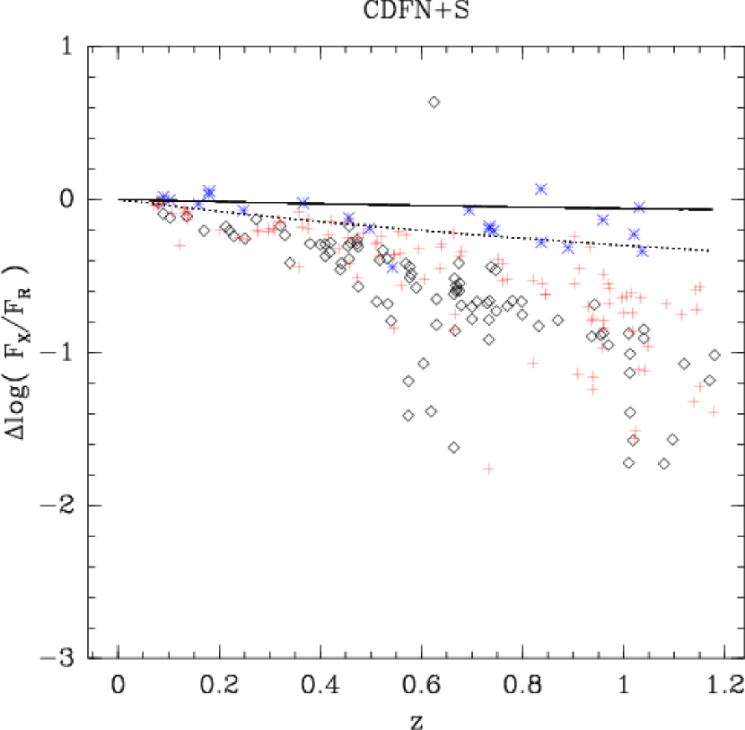
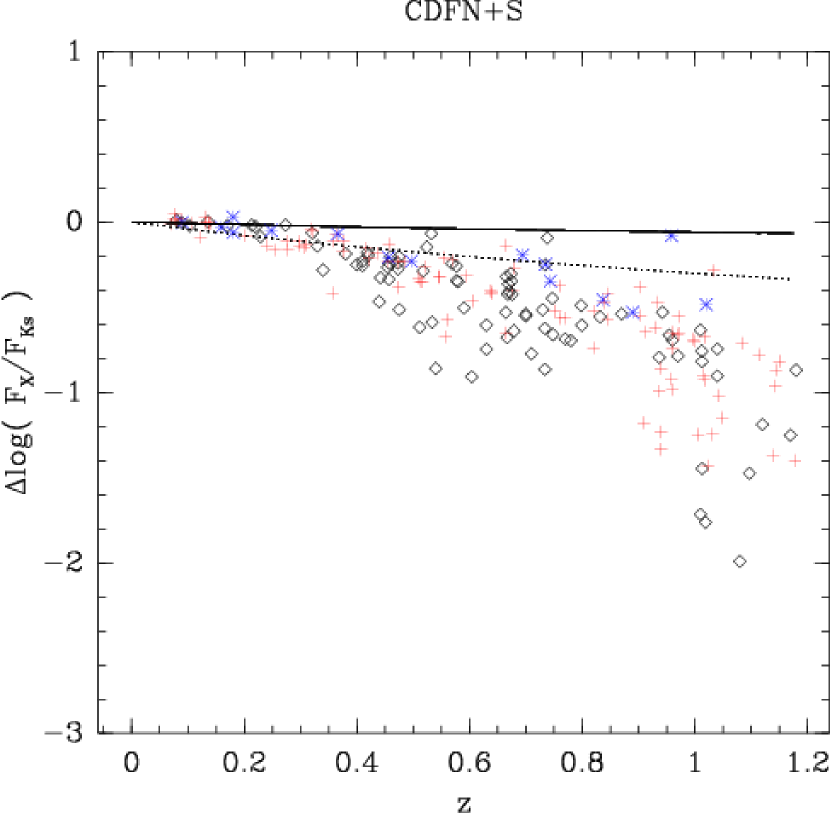
Figure 3.— The k-corrections applied to the X-ray flux ratios for the R (left) and $\rm K_{s}$ (right) bands, for both of the GOODS fields. The points show $\Delta\log[F_{X}/F_{opt}]=\log[(F_{X}/F_{opt})_{z=0}]-\log[(F_{X}/F_{opt})_{z}]$, where $\log[(F_{X}/F_{opt})_{z=0}]$ is the flux ratio after applying k-corrections and $\log[(F_{X}/F_{opt})_{z}]$ is the “observed” flux ratio. Early-type sources are marked with (black) diamonds, late-type sources are marked with (red) pluses, and irregular/starburst sources are marked with (blue) asterisks. The solid and dotted lines show the X-ray k-correction for $\Gamma=1.8$ and $\Gamma=1.0$, respectively.

2.3. Luminosity Function Estimation

We construct binned luminosity functions using the estimator described in Page & Carrera (2000). Briefly, this assumes negligible variation in both the luminosity function and its evolution across each $\Delta L\Delta V(z)$ bin, where $V(z)$ is the co-moving volume:

$$N\simeq\phi(L,z)\int^{L_{max}}_{L_{min}}\int^{z_{max}}_{z_{min}}C(L,z)V(z)dzdL$$ (1)

$N$ is the number of sources in the XLF bin bounded by $L_{min}$, $L_{max}$, $z_{min}$ and $z_{max}$, and $C(L,z)$ is a completeness correction. Note that $z_{max}$ is a function of luminosity since the limit is chosen at the highest observable redshift given the limiting flux (or, equivalently, $C(L,z)=0$ where $F(L,z)<F_{lim}$). The error for each XLF bin is accordingly derived from the Poisson error on the number of galaxies in each bin (note this assumes negligible statistical and systematic error in the volume integral terms), and for bins with no galaxies we used N=1.841 as the 1$\sigma$ upper limit (Gehrels, 1986). Small luminosity function bins are preferred, however larger bins minimize Poisson noise and reduce the effect of luminosity uncertainties within a bin (due to redshift uncertainties). For example, for the uncertainty in luminosity resulting from redshift error to be on the order of the bin size, bin sizes of $\Delta\log L=0.5$ are required for sources with $z\gtrsim 0.4$ and redshift errors of 0.1 or less. Given the small number of sources, we divide our sample into just two redshift bins, $z<0.5$ and $0.5<z<1.2$. We used the soft-band GOODS sky coverage shown in Treister et al. (2004).

2.4. Completeness Correction

The completeness correction $C(L,z)$ is given by the product of the X-ray detection completeness, the probability of a given X-ray source having an optical/NIR counterpart, and the probability of a counterpart having a redshift. The latter two terms reduce to the probability of an X-ray source having a redshift. For the X-ray detection completeness we used the results of simulations originally performed for the full CDF areas discussed in Bauer et al. (2004), where the effective solid angle for each source was computed (i.e., the maximum solid angle over which the source could have been detected). The ratio of the effective solid angle to the (total) CDF solid angle at the flux of the source is then an estimate of the completeness for sources at a similar flux and position. We then computed the completeness as a function of flux by multiplying the mean per-source completeness (i.e., effectively averaging over off-axis angle) and the fraction of GOODS x-ray sources with a redshift in the given flux range (the bin sizes were 0.5 dex for the GOODS-N sources and 0.75 dex for the GOODS-S sources), shown in Figure 4. In both the GOODS-N and GOODS-S the completenesses ranged from $\sim 60\%$ at $F_{0.5-2.0\rm\ keV}=2\times 10^{-17}$ erg cm^-2 s^-1in the North and $F_{0.5-2.0\rm\ keV}=7\times 10^{-17}$ in the South to 100% for $F_{0.5-2.0\rm\ keV}>10^{-14}$erg cm^-2 s^-1, although with errors on the order of 20% in each flux bin. We fit the completeness with a quadratic function, both to avoid the impact of statistical fluctuations and to have an analytic expression for use in calculating Eq. 1. The best-fitting relation was $C(F_{X})=14.56+1.66\log F_{X}+0.0495(\log F_{X})^{2}$ and is shown in Figure 4.

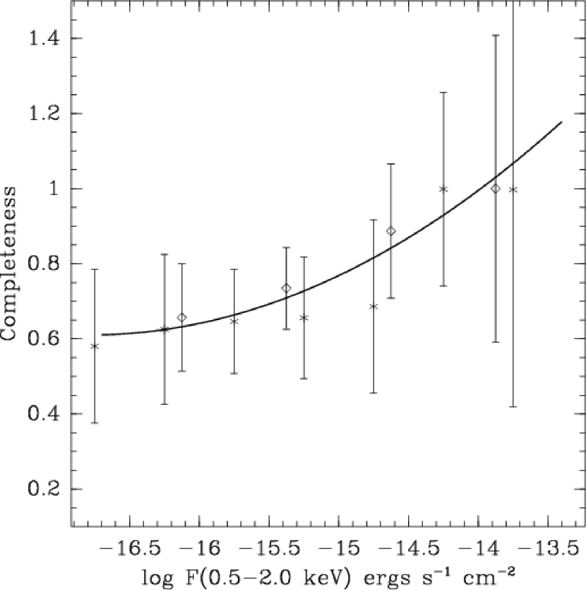
Figure 4.— Completeness corrections as a function of flux calculated for the GOODS-N (crosses) and GOODS-S (diamonds) regions. The line shows a quadratic fit to the combined completeness corrections (i.e., to be applied to either data set).

2.5. Galaxy Classification

N04 classified sources as AGN1 (broad-line AGN), AGN2 (narrow-line AGN), and “galaxy” (i.e., normal/starburst galaxy) using a prior based on the observed distributions of X-ray luminosity ($\log L_{X}$), the X-ray-to-optical flux ratio ($\log F_{X}+R$), and X-ray hardness ratio derived from a subset of the sources where the optical classification was secure. These distributions were used as priors along with the likelihoods of these measured values in computing the posterior probabilities. A source was then classified as a galaxy if the galaxy probability exceeded the AGN1 and AGN2 probabilities.

Here we employ a similar algorithm, discussed in Appendix A . However, there are a number of differences with the approach in N04, including use of the X-ray/K-band flux ratio, inclusion of k-corrections in the computation of X-ray/optical and X-ray/NIR flux ratios, and a more conservative galaxy selection threshold. Note that our priors are based on the spectroscopic data in Szokoly et al. (2004) which covers the entire CDF-S area. In Szokoly et al. only R and K band values are listed, and accordingly k-corrections could not be interpolated as was done with the GOODS data (see §2.2). However, we estimated the spectral type of the sources based on their R-K color, and applied a mean k-correction derived for each type.

In the case of X-ray hardness ratio, the means and standard deviations of the prior samples were $-0.19\pm 0.46$ for galaxies, $0.16\pm 0.37$ for AGN2 and $-0.51\pm 0.05$ for AGN1, very similar to those used in N04. For comparison, Peterson et al. (2006) artificially redshifted a sample of local galaxies to $z=0.3$ and found that hardness ratios of AGN2 was split evenly around HR=0. They noted that soft emission from starbursts could be resulting in HR$<$0 in AGN2/starburst composites (the case for 4 out of the 7 AGN2 with HR$<$0). Our final normal/starburst galaxy sample consisted of 64 CDF-N sources and 23 CDF-S sources. We also consider an “optimistic” normal/starburst galaxy sample which includes all sources that were not classified as an AGN. This sample therefore includes sources with ambiguous classification, similar to the original selection in N04. The optimistic normal/starburst sample contains 98 CDF-N and 54 CDF-S sources.

2.6. XLF Model Fitting

In order to quantify differences among the various XLFs discussed here, we fit the XLFs with several models (note that all luminosity functions discussed here are binned). The simplest model is a linear function in $\log\phi$-$\log L_{X}$ space, i.e., $\log\phi(L_{X})=a\log{L_{X}}+b$. We performed linear fits with two conventional approaches, namely using the survival analysis linear regression (hereafter Method 1) discussed in Isobe et al. (1986), and least-squares fitting (using the qdp program) after excluding the upper limits (Method 2). The linear regression approach has the disadvantage of not explicitly including any error information (i.e., the algorithm only takes as input the value of each detection or limit), and the confidence level used in computing an upper limit is arbitrary.

2.6.1 Markov-Chain Monte Carlo Fitting

Bayesian parameter estimation has been gaining popularity in various fields of astronomy, most notably in cosmology (see, e.g., Spergel, 2007). A key advantage of Bayesian parameter estimation is that common statistical issues, such as the treatment of upper limits in fitting and propagation of errors, are inherently handled properly. In addition the probability distributions for parameters of interest are computed and can be shown rather than simply a summary such as the 68% confidence interval. This latter point is particularly relevant when there are relative minima in the fitting statistic, in which case the meaning of traditional error bar is not well defined.

The basis of Bayesian parameter estimation is the computation of the posterior probability distribution:

$$p(\theta|D)=\frac{p(\theta)p(D|\theta)}{p(D)}$$ (2)

where $\theta$ is the vector of model parameters (e.g., $\theta=\{a,b\}$ for the linear model), $D$ represents the data, $p(\theta)$ is the prior probability distribution for the parameters, $p(D|\theta)$ is the likelihood function, and $p(D)$ is a normalization constant (i.e., since it does not depend on the parameter values). $p(D)$ is given by $\int p(\theta)p(D|\theta)d\theta$. In practice, computing $p(\theta|D)$ is computationally difficult since it requires an $n$-dimensional integral when fitting an $n$ parameter model. The Markov-chain Monte Carlo (MCMC) procedure circumvents this by performing a directed random walk through the parameter space (van Dyk et al., 2001; Ford, 2006). Here we assume Gaussian priors for each parameter (with mean and standard deviation $\mu_{\theta_{i}}$ and $\sigma_{\theta_{i}}$ for parameter $\theta_{i}$), and chose very large $\sigma_{\theta_{i}}$ values for the case of a flat (uninformative) prior. The likelihood function for the number of counts in an XLF bin is the Poisson distribution, giving

$$p(\theta|D)\propto\prod_{i=1}^{n}G(\theta_{i}|\mu_{\theta_{i}},\sigma_{\theta_{i}})\times\\ \times\prod_{j=1}^{m}Pois[N_{j}|\phi(\theta_{1},..,\theta_{n},L_{X,j},z_{j})V(L_{X,j},z_{j})]$$ (3)

where there are $n$ model parameters and $m$ XLF bins. $G(\theta_{i}|\mu_{\theta_{i}},\sigma_{\theta_{i}})$ is the Gaussian prior for parameter $\theta_{i}$. $N_{j}$ is the number of sources and $V(L_{X,j},z_{j})$ is the co-moving volume corresponding to the jth bin (see Eq. 1). $\phi(\theta_{1},..,\theta_{n},L_{X,j},z_{j})$ is the model XLF evaluated at $L_{X,j}$ and $z_{j}$. The $Pois[]$ terms give the likelihood of detecting $N_{j}$ galaxies in XLF bin $j$ given an expectation of $\phi V$. In addition to the simple linear model we also fitted Schechter and log-normal functions to the individual XLFs. We used the Metropolis-Hastings MCMC algorithm, in which a “proposal” distribution is used to guide the variation of the parameters (see Ford, 2005; Russell et al., 2007). In this procedure random offsets for each parameter are drawn from the proposal distribution, and accordingly the step sizes (i.e., the Gaussian $\sigma$s) are preferably on the order of the final error for that parameter. A step is accepted if the probability of the model given the new parameter values is higher, and also at random intervals when the probability is lower (i.e., occassionally the fit is allowed to proceed “downhill” to avoid relative minima). For a given run, three chains were produced with a length of at least $2\times 10^{6}$ iterations, and the parameter step sizes were adjusted during the first chain to achieve acceptance rates in the range 0.35-0.4. Only the last chain in a given run was used for analysis. At least 10 runs were performed for a given fit and we computed the convergence $R$ statistic from Gelman et al. (2004). $R$ values $\lesssim 1.2$ indicate convergence, and in every case the $R$ values were $<1.01$. In practice, the linear model parameters $a$ and $b$ were highly correlated, which leads to inefficient MCMC fitting. As discussed in Gelman et al. (2004), we addressed this by instead fitting for $a_{1}$, $a_{2}$ and $b$, where $a=a_{1}+a_{2}b$. The initial values of $a_{1}$ and $a_{2}$ were determined from a linear regression fit to the output of a short MCMC run, and the value of $a_{2}$ was held approximately fixed by using a tight prior ($a_{1}$ and $a_{2}$ are “nuisance” parameters and are not discussed further). The initial parameter values for a given run was chosen randomly and the range of the allowed values was $\pm 2\times$ the initial step size from the prior mean. The dispersion between the best-fitting parameter values from the runs in a given fit was always $<10\%$ of the final error in the parameters, showing that the chains converged independently of the starting values. For each parameter of interest the chain values were binned into normalized histograms, which represent the marginalized posterior probability distribution of the parameter. The peak value (i.e., the mode) was taken as the best-fit value and the 68% confidence interval was derived from the probability density by steeping from the peak in the direction of the smallest decrease until the integrated area equaled 68%, as discussed in Kraft et al. (1991). In order to assess how constraining the prior is, we computed the ratio of the prior $\sigma$ values to the standard deviation of the MCMC parameter values (i.e., the 68% error in the case of a Gaussian posterior probability distribution). In tables showing the fit results we marked parameter values and errors as having a tightly-constraining prior when this ratio is $<$1.1 and as a moderately-constraining prior when it is between 1.1 and 2.0.

2.6.2 Fit Quality

Unfortunately the MCMC procedure does not directly provide a model probability estimate since this requires the normalization of Eq. 2 to be computed. Since efficient model selection is complicated (and the subject of active research, see, e.g., Trotta 2007), we defer this and here we compute $\chi^{2}$ for the models after excluding upper limits. This also has the advantage that it can be consistently applied to all of the model fitting methods discussed here in the case of the linear model.

3. Results

3.1. Linear Model Fits

In Figures 5-9 we show the XLFs derived from the GOODS fields based on the early-type, late-type and total early + late-type galaxy samples along with the linear model fits. We also show the fits to the “optimistic” galaxy sample and the N04 XLFs for comparison. The best-fit parameters and errors are given in Table 1 along with the associated $\chi^{2}$ values and the probability with which the model can be rejected (again with the caveat that this probability does not include upper limit data).

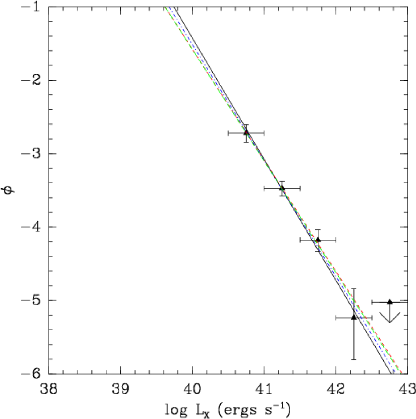
Figure 5.— Full-sample (early + late-type galaxy) XLFs from the GOODS fields, for the redshift intervals z$<$0.5 (left) and 0.5 $<$ z $<$ 1.2 (right). The solid (black), dashed (red), dot-dashed (blue) and long-dashed lines (green) lines respectively show the best-fitting models from Method 1 (survival analysis linear regression), Method 2 (least-squares excluding upper-limits), MCMC fitting with Method 1 results used to initialize the fit, and MCMC fitting with Method 2 results used to initialize the fit.

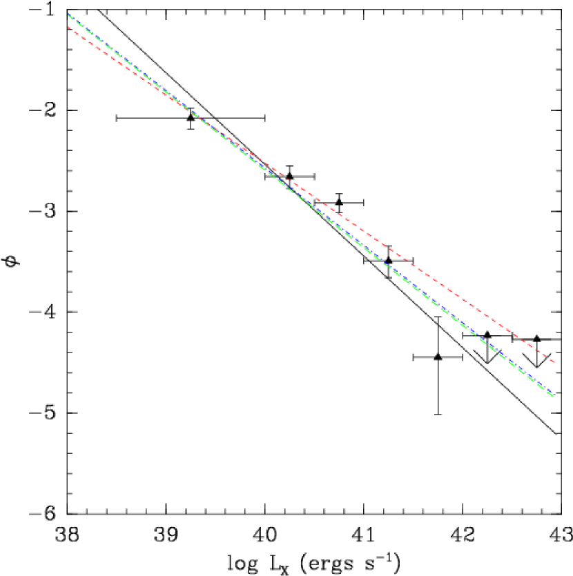
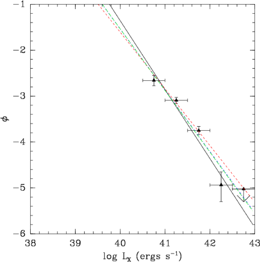
Figure 6.— “Optimistic” sample (early + late-type galaxy) XLFs from the GOODS fields, for the redshift intervals z$<$0.5 (left) and 0.5 $<$ z $<$ 1.2 (right). Lines are as in Figure 5

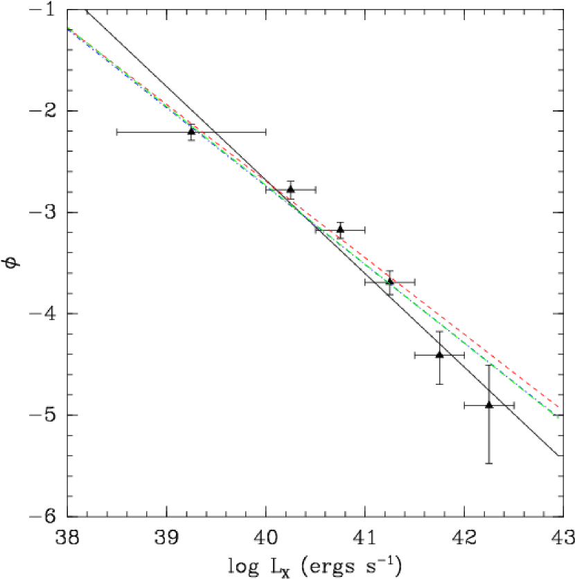
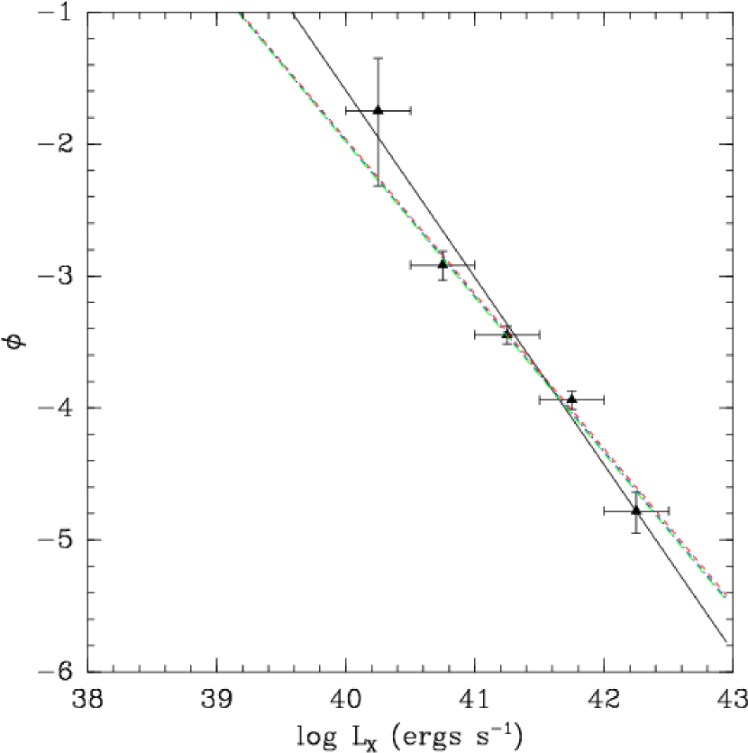
Figure 7.— The N04 XLFs for z$<$0.5 (left) and 0.5 $<$ z $<$ 1.2 (right), with linear fits shown as in Figure 5.

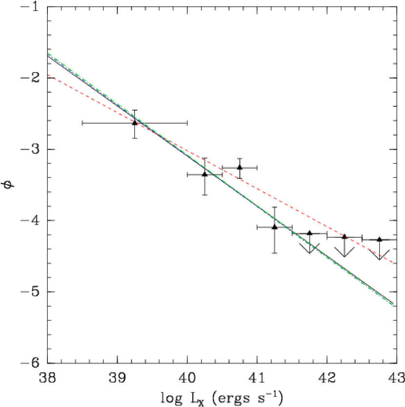
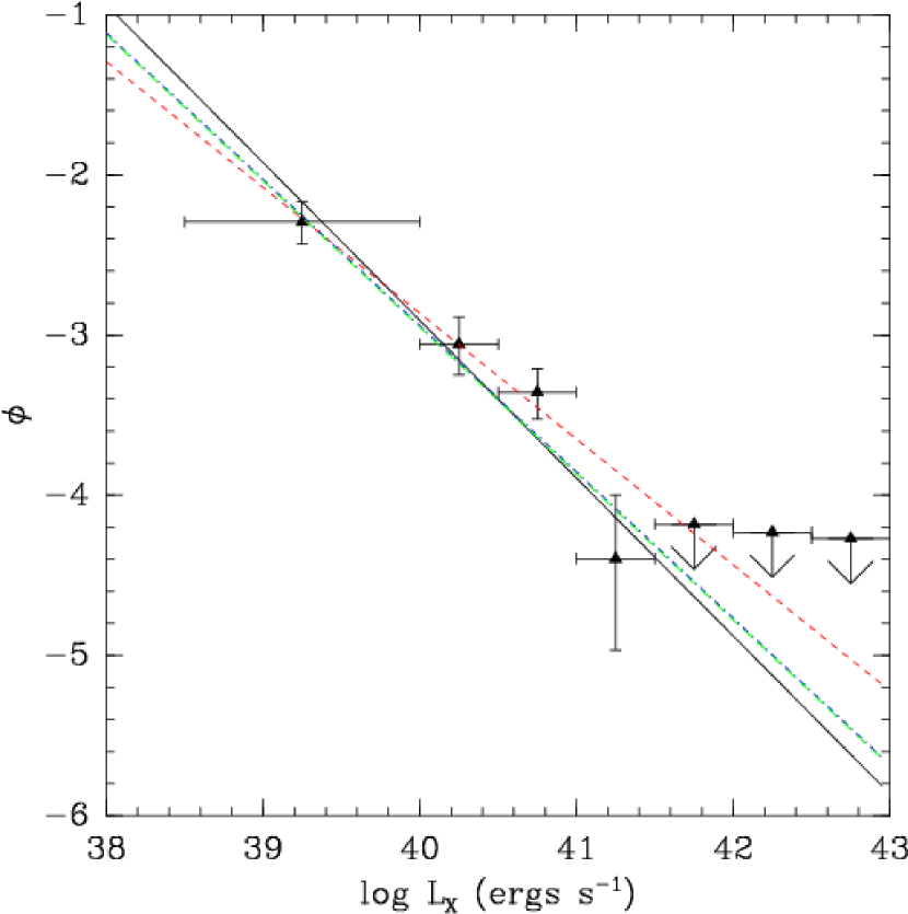
Figure 8.— $z<0.5$ early-type (left) and late-type (right) galaxy XLFs from the GOODS fields. Lines are as in Figure 5.

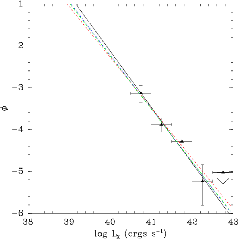
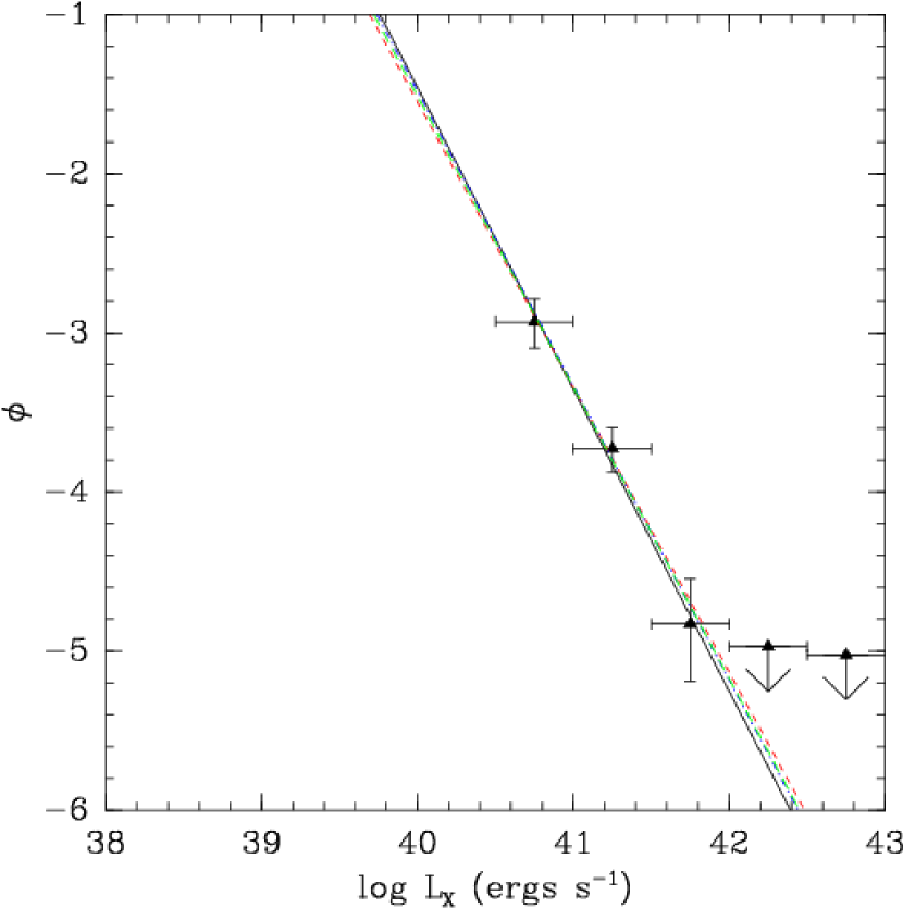
Figure 9.— $0.5<z<1.2$ early-type (left) and late-type (right) galaxy XLFs from the GOODS fields. Lines are as in Figure 5.

Table 1XLF Linear Fits

Sample	Method	$a$	$b$	$\chi^{2}/dof$	$p_{\chi^{2}}$
Early-type galaxies, low-z	1	$-0.70\pm 0.11$	$25.0\pm 4.5$	3.58/2	83.2%
	2	$-0.53^{+0.13}_{-0.13}$	$18.3^{+5.4}_{-5.4}$	6.34/2	95.6%
	3*	$-0.71^{+0.12}_{-0.09}$	$25.4^{+5.2}_{-3.3}$	3.66/2	83.9%
	3†	$-0.72^{+0.11}_{-0.10}$	$25.6^{+5.2}_{-3.3}$	3.70/2	84.2%
Late-type galaxies, low-z	1	$-0.99\pm 0.14$	$36.5\pm 5.5$	3.78/2	84.8%
	2	$-0.79^{+0.11}_{-0.12}$	$28.6^{+4.7}_{-4.6}$	5.55/2	93.6%
	3*	$-0.91^{+0.09}_{-0.11}$	$33.6^{+4.1}_{-3.9}$	2.95/2	77.0%
	3†	$-0.91^{+0.12}_{-0.08}$	$33.6^{+4.1}_{-4.0}$	2.97/2	77.2%
All galaxies, low-z	1	$-0.90\pm 0.11$	$33.5\pm 4.6$	8.95/2	98.6%
	2	$-0.67^{+0.09}_{-0.08}$	$24.1^{+3.4}_{-3.5}$	12.47/2	99.5%
	3*	$-0.81^{+0.06}_{-0.08}$	$29.8^{+3.3}_{-2.3}$	6.64/2	96.2%
	3†	$-0.82^{+0.06}_{-0.08}$	$30.1^{+3.1}_{-2.5}$	6.64/2	96.2%
All galaxies (optimistic), low-z	1	$-0.91\pm 0.11$	$33.8\pm 4.6$	15.98/3	99.9%
	2	$-0.67^{+0.07}_{-0.07}$	$24.4^{+2.9}_{-2.9}$	19.03/3	$>$99.9%
	3*	$-0.77^{+0.06}_{-0.06}$	$28.1^{+2.4}_{-2.4}$	9.85/3	98.0%
	3†	$-0.77^{+0.06}_{-0.06}$	$28.2^{+2.2}_{-2.5}$	9.70/3	97.9%
Norman et al. (2004), low-z	1	$-0.92\pm 0.07$	$34.2\pm 2.8$	20.24/4	$>$99.9%
	2	$-0.76^{+0.05}_{-0.05}$	$27.5^{+2.2}_{-2.1}$	13.85/4	99.2%
	3*	$-0.77^{+0.05}_{-0.04}$	$28.2^{+2.0}_{-1.8}$	10.56/4	96.8%
	3†	$-0.78^{+0.04}_{-0.06}$	$28.4^{+1.7}_{-2.1}$	10.43/4	96.6%
Early-type galaxies, hi-z	1	$-1.34\pm 0.10$	$51.5\pm 4.2$	1.17/2	44.4%
	2	$-1.21^{+0.21}_{-0.21}$	$46.2^{+8.7}_{-8.7}$	1.25/2	46.3%
	3*	$-1.28^{+0.20}_{-0.21}$	$49.0^{+9.1}_{-8.0}$	1.07/2	41.4%
	3†	$-1.27^{+0.18}_{-0.23}$	$48.4^{+9.5}_{-7.5}$	1.07/2	41.3%
Late-type galaxies, hi-z	1	$-1.90\pm 0.10$	$74.5\pm 4.2$	0.58/1	53.9%
	2	$-1.79^{+0.29}_{-0.29}$	$70.1^{+11.7}_{-11.7}$	0.52/1	51.5%
	3*	$-1.85^{+0.29}_{-0.23}$	$72.6^{+12.4}_{-8.8}$	0.54/1	52.3%
	3†	$-1.83^{+0.19}_{-0.32}$	$71.7^{+13.0}_{-8.1}$	0.49/1	50.5%
All galaxies, hi-z	1	$-1.65\pm 0.08$	$64.6\pm 3.3$	0.99/2	38.9%
	2	$-1.51^{+0.16}_{-0.16}$	$58.9^{+6.7}_{-6.7}$	0.62/2	26.8%
	3*	$-1.58^{+0.17}_{-0.14}$	$61.7^{+5.7}_{-7.3}$	0.64/2	27.2%
	3†	$-1.52^{+0.13}_{-0.18}$	$59.3^{+8.1}_{-4.9}$	0.60/2	25.9%
All galaxies (optimistic), hi-z	1	$-1.50\pm 0.17$	$58.7\pm 6.9$	11.75/2	99.4%
	2	$-1.24^{+0.12}_{-0.12}$	$47.8^{+5.1}_{-5.1}$	13.83/2	99.6%
	3*	$-1.33^{+0.11}_{-0.09}$	$51.8^{+4.3}_{-4.1}$	9.16/2	98.7%
	3†	$-1.34^{+0.10}_{-0.10}$	$52.2^{+3.9}_{-4.5}$	9.12/2	98.7%
Norman et al. (2004), hi-z	1	$-1.42\pm 0.10$	$55.1\pm 4.2$	15.25/3	99.8%
	2	$-1.17^{+0.09}_{-0.09}$	$45.0^{+3.9}_{-3.9}$	4.10/3	74.9%
	3*	$-1.18^{+0.10}_{-0.09}$	$45.1^{+3.6}_{-4.1}$	3.76/3	71.1%
	3†	$-1.18^{+0.08}_{-0.10}$	$45.2^{+3.6}_{-4.2}$	3.76/3	71.2%

Note. — Fit parameters are given for $\log\phi=a\log L_{X}+b$. Method 1: linear regression, 2: fit to data excluding upper-limits, 3*: MCMC fit using Method 1 results to initialize the fit, 3^†: MCMC fit using Method 2 results to initialize the fit (see text). $p_{\chi^{2}}$ gives the $\chi^{2}$ probability at which the model fit can be rejected (note that $\chi^{2}$ is computed excluding upper limits).

As is evident from the fit results, the MCMC fitting was not very sensitive as to whether the Method 1 or Method 2 fit values were used as the prior means. Interestingly, in every case the MCMC fits resulted in curves that were intermediate to the Method 1 and Method 2 fits, and tended towards the Method 1 results when upper-limits were constraining (e.g., the early-type and late-type galaxy XLFs) and towards Method 2 when the no upper limits were used or the upper limits were not constraining (e.g., the Normal et al XLFs). The marginalized posterior probability distributions for $a$ and $b$ were close to Gaussian, resulting in nearly symmetric errors. In general the linear models cannot be rejected at high confidence (i.e., $>3\sigma$). Hereafter, the fit results presented refer to MCMC fitting.

3.2. Joint Linear Model Fits

In Figures 10-11 we show the results of fitting corresponding pairs of XLFs simultaneously (i.e., the low and high redshift XLFs for a given sample, and the early and late-type galaxy XLFs at low or high redshift), explicitly fitting for the offsets in $a$ and $b$ between the XLFs. Figure 12 shows the early and late-type XLFs similarly being fitted jointly. Here also the posterior probabilities were mostly Gaussian in shape, and the best-fit parameter values and errors are given in Table 2. These fits resulted in parameters for the given XLFs that were equivalent to those obtained by fitting the XLFs seperately with the linear model, however here we are deriving the probability distribution for the offsets in slope and intercept. As discussed above, this approach avoids the need to propagate errors in determining the significance of the change in the linear model parameters between XLFs. However, in these fits the final errors on $\Delta a$ and $\Delta b$ are very similar to adding the errors obtained from the individual fits in quadrature, which is perhaps not surprising given that the posterior probabilities for these parameters were nearly Gaussian. In every case, the best fit values of $\Delta a$ were $<0$ and the best fit values of $\Delta b$ were $>0$. In order to estimate the significance of a change in the XLF, we determined the fraction of simulations in which $\Delta a<0$ and $\Delta b>0$. Since in some cases this probability is very small, we performed 50 runs with a very large chain length ($5\times 10^{6}$) for these fits. These probabilities are also listed in Table 2.

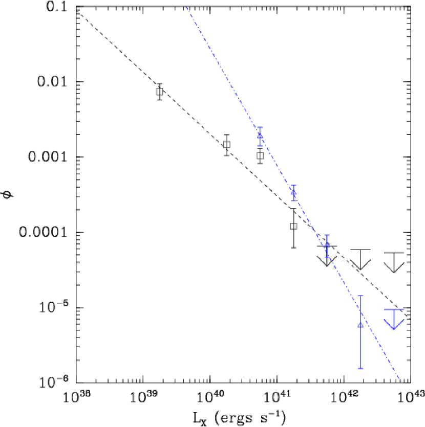
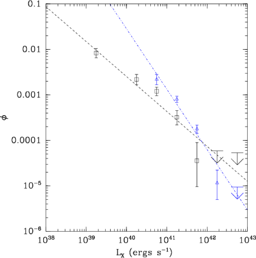
Figure 10.— Joint linear fits to the low-z and high-z XLFs for the full (early + late-type) galaxy sample (left) and the optimistic galaxy sample (right). The low-z XLF points are marked with (black) squares and the high-z XLF points are marked with (blue) triangles. The dashed (black) lines and dot-dashed (blue) lines respectively show the fit to the low-z and high-z XLFs.

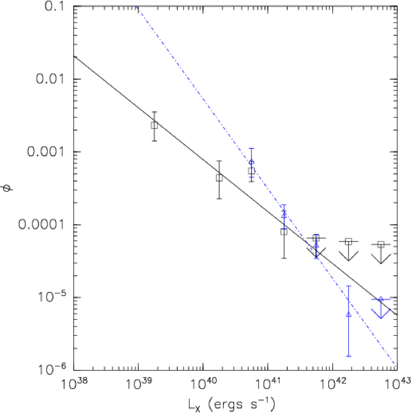
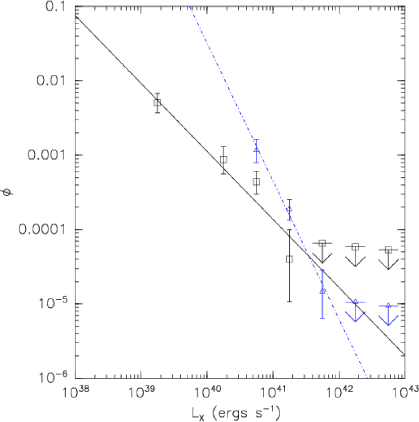
Figure 11.— As in Figure 10, with the left panel showing the early-type galaxy XLFs and the right panel showing the late-type galaxy XLFs.

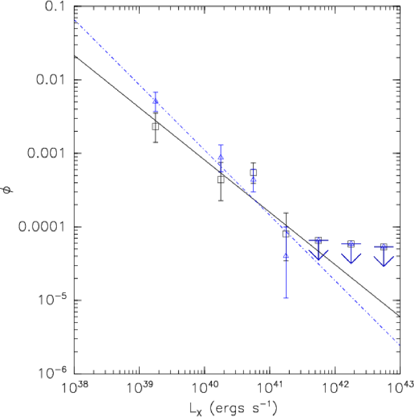
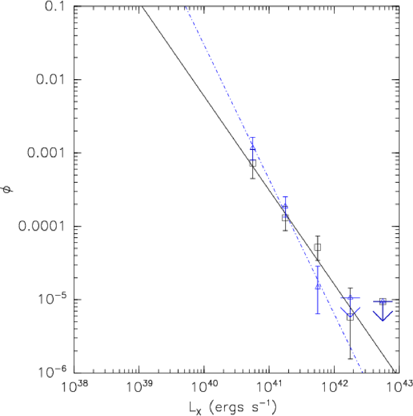
Figure 12.— Joint linear fits to the low-z early and late-type XLFs (left) high-z early and late-type XLFs (right). The early-type XLF points are marked with (black) squares and the late-type XLF points are marked with (blue) triangles. The dashed (black) lines and dot-dashed (blue) lines show the fit to the early and late-type XLFs.

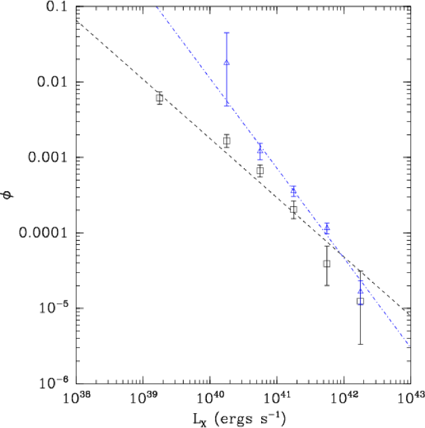
Figure 13.— As in Figure 10 for the N04 XLFs.

Table 2MCMC Joint Linear Fits

Sample	$\Delta a$	$\Delta b$	$p_{\Delta a,\Delta b}$	$\chi^{2}/dof$	$p_{\chi^{2}}$
All galaxies	$-0.75^{+0.19}_{-0.15}$	$30.4^{+6.9}_{-7.2}$	$>$99.9%	7.3/4	87.9%
All galaxies (optimistic)	$-0.56^{+0.10}_{-0.13}$	$23.5^{+5.1}_{-4.5}$	$>$99.9%	18.9/5	99.8%
Norman et al. (2004)	$-0.38^{+0.09}_{-0.11}$	$17.0^{+3.9}_{-4.7}$	$>$99.9%	14.0/7	94.9%
Early-type galaxies	$-0.58^{+0.25}_{-0.21}$	$21.6^{+11.4}_{-7.7}$	99.4%	4.7/4	68.4%
Late-type galaxies	$-1.03^{+0.33}_{-0.23}$	$39.1^{+12.8}_{-9.9}$	$>$99.9%	3.5/3	67.4%
Early/late-type galaxies, low-z	$-0.19^{+0.15}_{-0.14}$	$7.2^{+6.0}_{-5.6}$	89.8%	6.6/4	84.4%
Early/late-type galaxies, hi-z	$-0.59^{+0.32}_{-0.34}$	$22.8^{+15.4}_{-11.7}$	96.9%	1.6/3	33.2%

Note. — Best-fitting change in slope ($\Delta a$) and intercept ($\Delta b$) from joint fits to the low and high-z samples. The ”Early/late-type” samples refer to comparing the early and late-type galaxy sample (i.e., see Figure 12). $p_{\Delta a,\Delta b}$ refers to the probability that $\Delta a<0$ and $\Delta b>0$.

$p_{\chi^{2}}$ gives the $\chi^{2}$ probability at which the model fit can be rejected (note that $\chi^{2}$ is computed excluding upper limits).

3.3. Log-Normal and Schechter Fits

We fit the XLFs using the log-normal (Saunders et al. 1990) and Schechter (Schechter et al. 1976) functions since these functional forms fit the FIR (and hence star-forming galaxy) and optical luminosity functions of galaxies well. Specifically the functional forms were:

$$\phi(L)=\phi^{*}\left(\frac{L}{L^{*}}\right)^{1-\alpha}\exp\left[-\frac{1}{2\sigma^{2}}\log^{2}(1+\frac{L}{L^{*}})\right]$$ (4)

$$\phi(L)=\ln(10)\phi^{*}\left(\frac{L}{L^{*}}\right)^{1+\alpha}\exp\left(-\frac{L}{L^{*}}\right)$$ (5)

where in both cases the units of $\phi$ are galaxies Mpc^-3 log$L^{-1}$. For both of these sets of fits we placed very weak priors on $\log L^{*}$ and $\log\phi^{*}$. We first fitted the FIR LF published in Saunders et al. (1990) in order to obtain prior information based on the local star-forming galaxy luminosity function, and to validate our methodology. We assumed that the errors listed for each LF point were Gaussian and excluded upper limits. Our results are shown in Table 3, along with the original results of Saunders et al. (1990) and the results of fitting the log-normal function to a more recent FIR sample in Takeuchi et al. (2001). Our results are consistent with the fitting based on traditional methods within the errors. Since the Takeuchi et al. LF fits were based on more recent data we set the log-normal fit prior means to their values, with $\log L^{*}$ scaled to the X-ray band using $\log L_{X}=\log L_{60\ \rm\mu m}-3.65$ (Ranalli et al. 1990), and by $(1+z)^{3}$ where $z=0.25$ for the $z<0.5$ XLFs and $z=0.75$ for the $0.5<z<1.2$ XLFs. In the case of the early-type or late-type galaxy XLFs we further reduced the prior mean for $\phi^{*}$ by a factor of 2 since these samples were $\sim 50\%$ of the total galaxy sample. We conservatively assumed the MCMC errors in Table 3 which were similar to, but larger than, the Takeuchi et al. errors. We set the prior standard deviations to 5 times these errors for $\alpha$ and $\sigma$ and 50 times these errors for $\log L^{*}$ and $\log\phi^{*}$ (effectively weak). In practice, however, different values of $\alpha$ were preferred by the data, and so we refit the data after setting the prior mean (and initial starting values) to the best-fitting $\alpha$ values from the original fits. The fits were not stable if we allowed the slope prior widths to be broader, and in the case of the early-type galaxy XLFs, the prior for $\alpha$ was required to be 50% smaller in order to result in stable fits.

Table 3Log-Normal Fits to the 60 $\mu$m Luminosity Function

Parameter	Saunders et al. (1990)	Takeuchi et al. (2001)	MCMC (This Work)
$\alpha$	$1.09\pm 0.12$	$1.23\pm 0.04$	$1.04^{+0.07}_{-0.08}$
$\sigma$	$0.724\pm 0.031$	$0.724\pm 0.010$	$0.751^{+0.014}_{-0.015}$
$\phi\ h^{3}\rm\ Mpc^{-3}$	$0.026\pm 0.008$	$0.026\pm 0.003$	$0.026^{+0.003}_{-0.003}$
$L^{*}\ h^{-2}\rm\ L_{\odot}$	$10^{8.47\pm 0.23}$	$(4.34\pm 0.86)\times 10^{8}$	$10^{8.39^{+0.12}_{-0.15}}$

Note. — The data used in our MCMC fitting of the 60 $\mu$m LF was taken from Saunders et al. (1990), with several upper-limit data points excluded.

The log-normal XLF fits to the XLFs are shown in Figures 14-18, with the best-fit parameters and errors given in Table 4. The posterior probability distributions for the fit parameters for the $z<0.5$ early-type sample XLF are shown in Figure 19, and the probability distributions for the fit parameters from the other log-normal fits have similar shapes. Note that using a tighter prior for $\alpha$ for the early-type galaxy fits did not change the best-fit parameter values significantly but resulted in $\sim 25\%$ smaller errors for $\log L^{*}$ and $\log\phi^{*}$. The posterior probability distributions for $\sigma$ were obviously completely dominated by the prior distribution. This is, nevertheless, an improvement over simply “fixing” fit parameters, which is the common procedure when parameters are not sufficiently constrained by the data since the width of the priors are scaled from the “physical prior” of the 60 $\mu$m LF fit results. A broad tail in the probability densities toward low values of $\log\phi^{*}$ and high values of $\log L^{*}$ is due to degeneracy between these parameters. This also can be seen in Figure 20 where the MCMC draws are plotted.

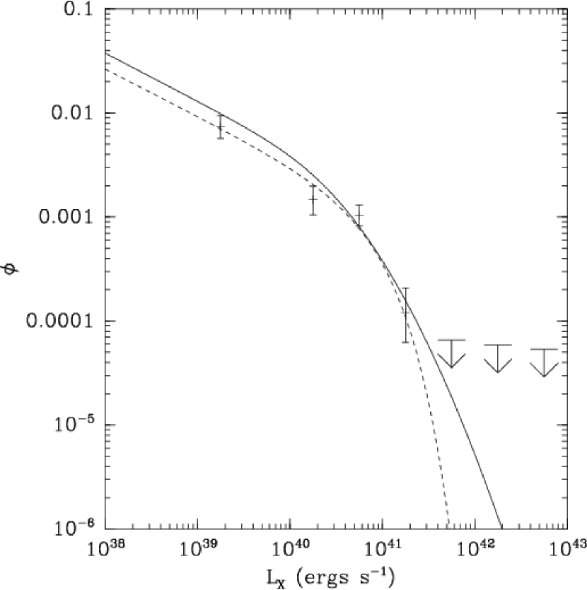
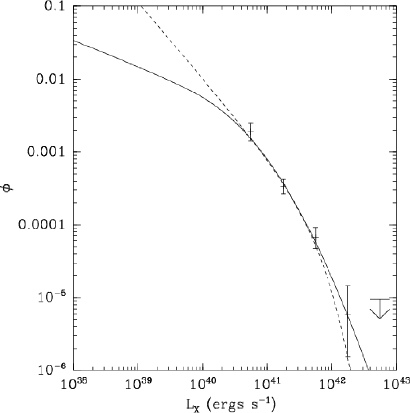
Figure 14.— Log-normal (solid curves) and Schechter function (dashed curves) fits to the full (early + late-type) galaxy sample. The left panel shows the $z<0.5$ sample and the right panel shows the $0.5<z<1.2$ sample.

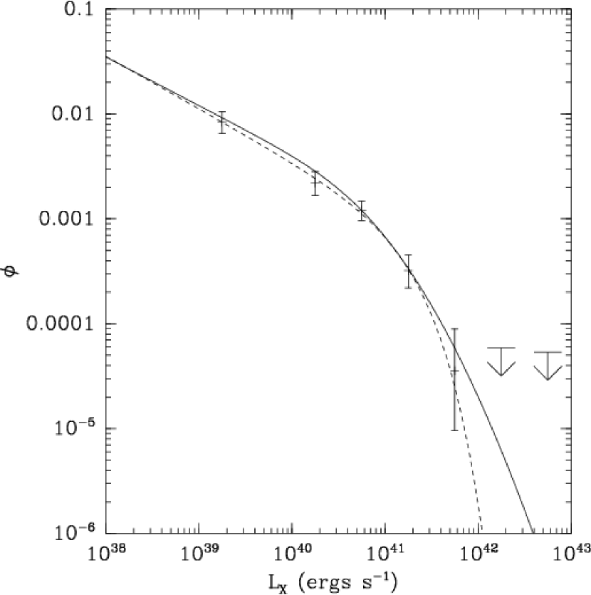
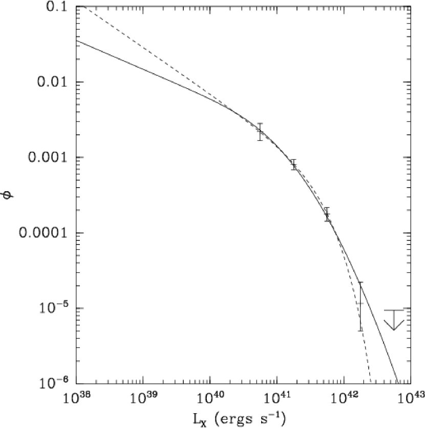
Figure 15.— Log-normal (solid curves) and Schechter function (dashed curves) fits to the optimistic galaxy sample. The left panel shows the $z<0.5$ sample and the right panel shows the $0.5<z<1.2$ sample.

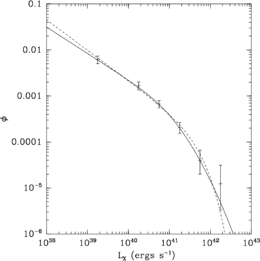
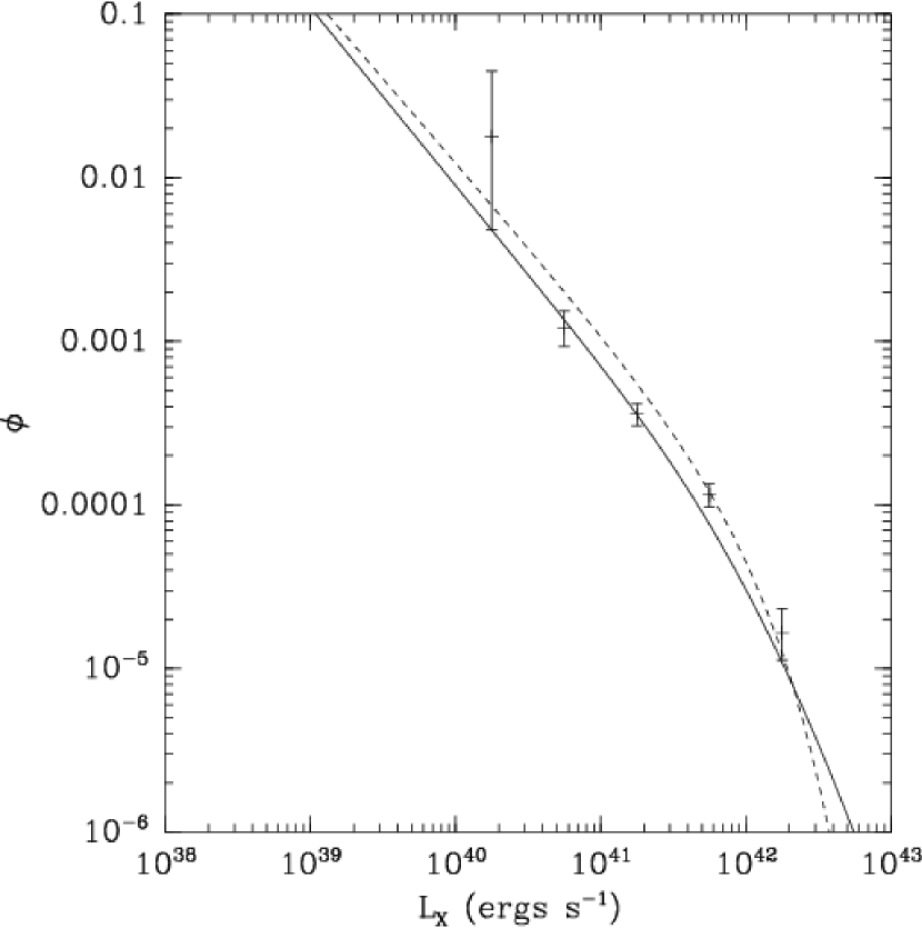
Figure 16.— Log-normal (solid curves) and Schechter function (dashed curves) fits to the N04 galaxy sample. The left panel shows the $z<0.5$ sample and the right panel shows the $0.5<z<1.2$ sample.

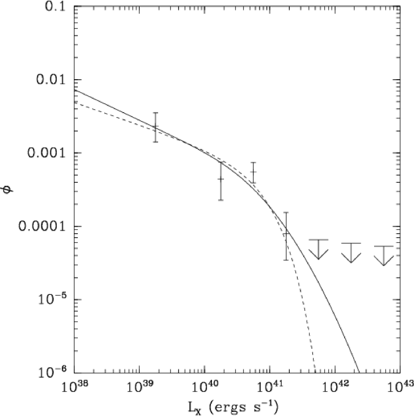
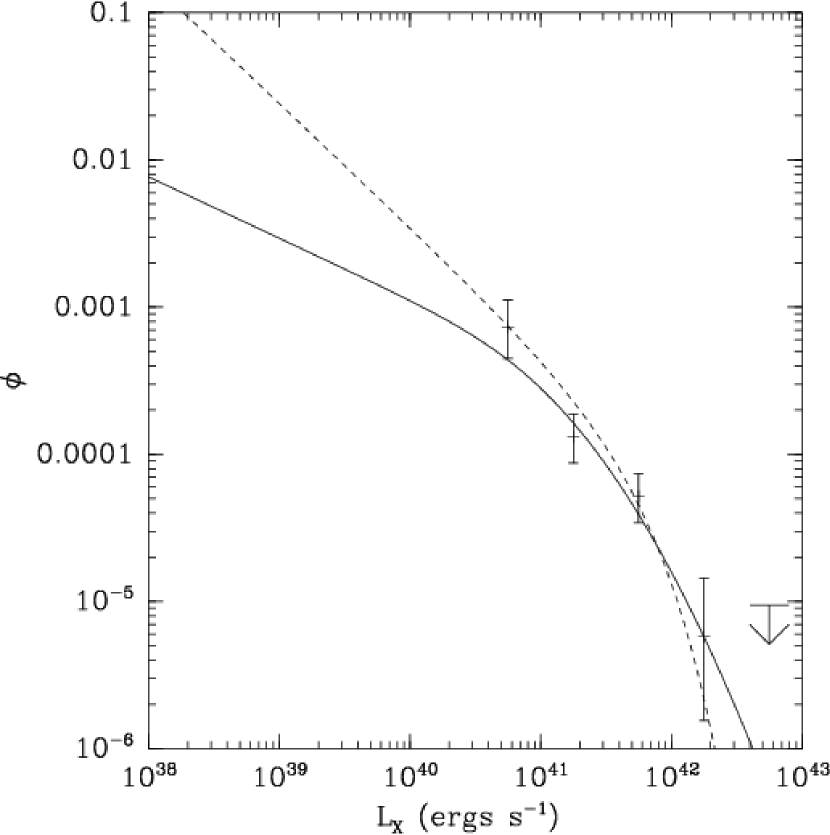
Figure 17.— Log-normal (solid curves) and Schechter function (dashed curves) fits to the early-type galaxy sample. The left panel shows the $z<0.5$ sample and the right panel shows the $0.5<z<1.2$ sample.

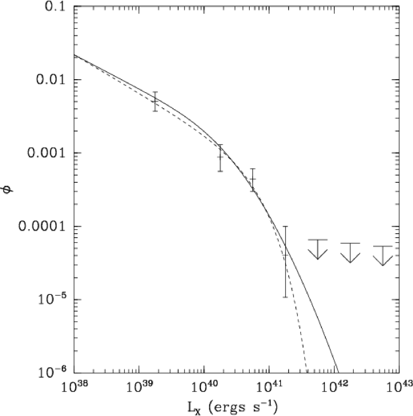
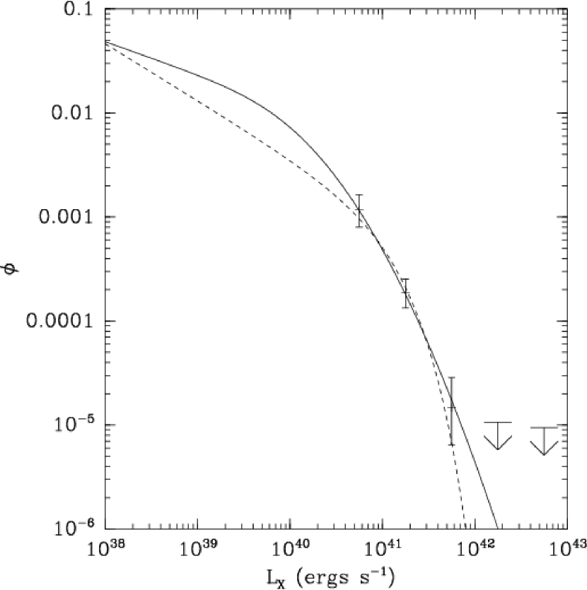
Figure 18.— Log-normal (solid curves) and Schechter function (dashed curves) fits to the late-type galaxy sample. The left panel shows the $z<0.5$ sample and the right panel shows the $0.5<z<1.2$ sample.

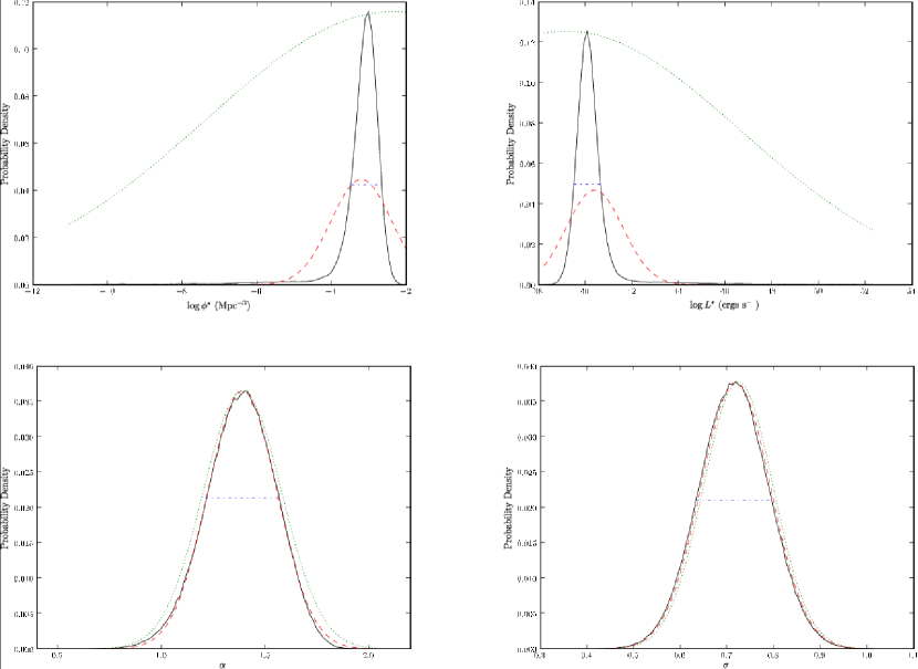
Figure 19.— Marginalized posterior probabilities for the fit parameters $\log\phi^{*}$, $\log L^{*}$, $\alpha$ and $\sigma$ for the log-normal fit to the $z<0.5$ early-type galaxy XLF. The solid (black) lines show the posterior probability, the dotted (green) line show the prior, the dashed (red) lines shows a Gaussian distribution with the same mean and standard deviation as the posterior, and the dot-dashed line shows the 68% confidence interval.

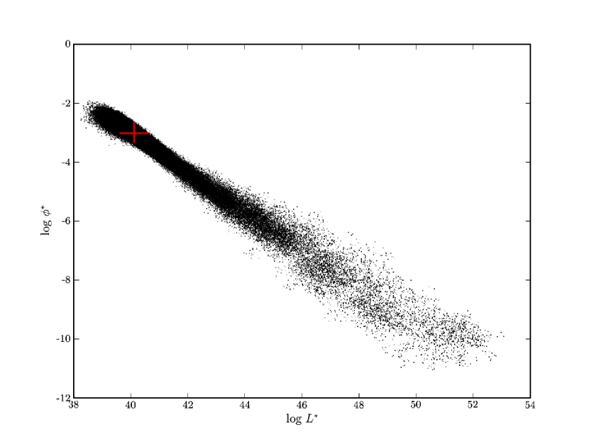
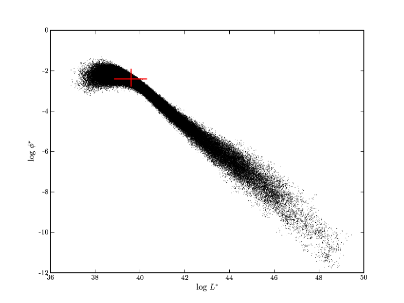
Figure 20.— The $z<0.5$ early-type (left) and late-type (right) galaxy MCMC draws for $\log\phi^{*}$ and $\log L^{*}$ in the log-normal fit. The solid lines show the 68% confidence intervals determined from the marginalized (and hence one-dimensional) posterior probabilities for the parameters.

Table 4MCMC Log-Normal Fits

Sample	$\log\phi^{*}$	$\log L^{*}$	$\alpha$	$\sigma$	$\log\rho$	$\chi^{2}/dof$	$p_{\chi^{2}}$
All galaxies, low-z	$-2.28^{+0.18}_{-0.39}$	$39.84^{+0.57}_{-0.43}$	$1.46^{+0.20}_{-0.26}$‡	$0.71^{+0.08}_{-0.07}$†	$37.94^{+0.07}_{-0.09}$	8.1	N/A
All galaxies (optimistic), low-z	$-2.46^{+0.31}_{-0.27}$	$40.17^{+0.44}_{-0.49}$	$1.46^{+0.17}_{-0.19}$‡	$0.73^{+0.08}_{-0.07}$†	$38.11^{+0.07}_{-0.08}$	1.8/1	79.9%
Norman et al. (2004), low-z	$-2.88^{+0.34}_{-0.38}$	$40.40^{+0.51}_{-0.40}$	$1.57^{+0.15}_{-0.10}$	$0.74^{+0.08}_{-0.07}$†	$37.96^{+0.08}_{-0.07}$	0.5/2	21.7%
Early-type galaxies, low-z	$-3.03^{+0.36}_{-0.30}$	$40.13^{+0.48}_{-0.47}$	$1.42^{+0.14}_{-0.19}$‡	$0.74^{+0.06}_{-0.09}$†	$37.62^{+0.13}_{-0.16}$	3.0	N/A
Late-type galaxies, low-z	$-2.41^{+0.34}_{-0.47}$	$39.61^{+0.74}_{-0.67}$	$1.46^{+0.35}_{-0.30}$‡	$0.73^{+0.07}_{-0.08}$†	$37.63^{+0.12}_{-0.10}$	1.6	N/A
All galaxies, hi-z	$-2.14^{+0.48}_{-0.48}$	$39.85^{+0.68}_{-0.60}$	$1.36^{+0.45}_{-0.36}$†	$0.75^{+0.07}_{-0.08}$†	$38.27^{+0.24}_{-0.17}$	0.9	N/A
All galaxies (optimistic), hi-z	$-2.34^{+0.27}_{-0.31}$	$40.32^{+0.52}_{-0.48}$	$1.38^{+0.37}_{-0.34}$†	$0.71^{+0.08}_{-0.07}$†	$38.44^{+0.14}_{-0.10}$	1.2	N/A
Norman et al. (2004), hi-z	$-3.4^{+1.0}_{-2.2}$	$41.2^{+2.1}_{-1.3}$	$2.09^{+0.16}_{-0.27}$‡	$0.73^{+0.08}_{-0.07}$†	$38.22^{+0.56}_{-0.09}$	6.0/1	94.1%
Early-type galaxies, hi-z	$-3.13^{+0.54}_{-0.40}$	$40.43^{+0.42}_{-0.60}$	$1.42^{+0.20}_{-0.20}$†	$0.73^{+0.08}_{-0.07}$†	$37.83^{+0.16}_{-0.13}$	1.6	N/A
Late-type galaxies, hi-z	$-1.76^{+0.81}_{-0.66}$	$39.43^{+0.57}_{-0.79}$	$1.32^{+0.40}_{-0.37}$†	$0.72^{+0.08}_{-0.06}$†	$38.24^{+0.34}_{-0.35}$	0.1	N/A

Note. — Best-fitting parameters from fitting a Log-Normal function to the XLFs.

^† Parameter is tightly constrained by prior

^‡ Parameter is moderately constrained by prior

Luminosities are in ergs s^-1 in the 0.5-2.0 keV bandpass.

$\rho$ is in ergs s^-1 Mpc^-3 in the 0.5-2.0 keV bandpass.

$p_{\chi^{2}}$ gives the $\chi^{2}$ probability at which the model fit can be rejected (note that $\chi^{2}$ is computed excluding upper limits).

We computed the luminosity density, $\rho=\int\phi(L)Ld\log L$, for each MCMC draw by numerically integrating the log-normal function over the range $10^{37}<L_{X}<10^{43}$ erg s^-1. The posterior probabilities for $\rho$ are shown in Figure 21. Note that this results in a statistically-correct estimation of $\rho$ and its error since no (usually questionable) propagation of errors is required.

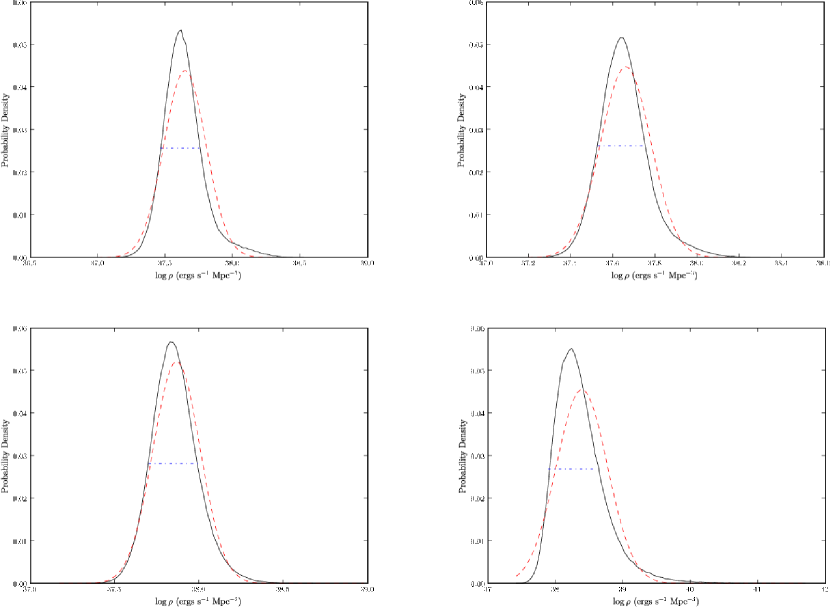
Figure 21.— The posterior probability distributions for the luminosity density ($\rho$) derived from log-normal fits to the early-type (left panels) and late-type (right panels) galaxy samples. The $z<0.5$ results are shown in the top row and the $0.5<z<1.2$ results are shown in the bottom row. The lines are as shown in Figure 19 (there is no prior for $\rho$ since it is derived from other fit parameters).

In the case of the Schechter function fits we assumed $\alpha=1.0$ with a prior width of $50$% (i.e., prior $\mu_{\sigma}=-1.0,\sigma_{\alpha}=0.5$) since the GOODS-S J-band $0.1<z<0.5$ luminosity function $\alpha$ values where in the range $-1.4<\alpha<-0.5$ (Dahlen et al. 2005). We also used the early-type galaxy $0.1<z<0.5$ J-band LF fit parameters from Dahlen et al. (2005) for $M_{J}^{*}$ (-22.97) and $\phi^{*}$ ($8.6\times 10^{-4}\rm\ Mpc^{-3}\ mag^{-1}$) to estimate the initial XLF fit parameters (and prior mean values) for $\log L^{*}$ and $\phi^{*}$. We converted $M_{J}$ to the X-ray band by computing the mean k-corrected value of $\log F_{X}+0.4J+5.1$ (see also Appendix C) to be -3.3 for normal galaxies. $\phi^{*}$ was rescaled by 2.5 to be in the units of Mpc^-3 dex^-1. As with the log-normal fits the prior mean for $\phi^{*}$ was reduced by a factor of 2 for the early-type and late-type galaxy sample XLFs. The best-fitting Schechter models are also shown in Figures 14-18, with the best-fitting parameter values and errors given in Table 5. The posterior probability densities for $\log L^{*}$, $\log\phi^{*}$, $\alpha$ and $\rho$ are shown in Figure 22 for the $z<0.5$ early-type galaxy sample, and again other Schechter fits resulted in posterior probabilities with roughly similar shapes.

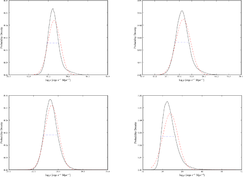
Figure 22.— Marginalized posterior probabilities for the fit parameters $\log\phi^{*}$, $\log L^{*}$, and $\alpha$ for the Schechter function fit to the $z<0.5$ early-type galaxy XLF. Also shown is the probability distribution for the luminosity density $\rho$ derived from the fit parameters. Lines are as shown in Figure 19.

Table 5MCMC Schechter Fits

Sample	$\log\phi^{*}$	$\log L^{*}$	$\alpha$	$\log\rho$	$\chi^{2}/dof$	$p_{\chi^{2}}$
All galaxies, low-z	$-3.27^{+0.28}_{-0.26}$	$40.93^{+0.24}_{-0.15}$	$-1.45^{+0.16}_{-0.12}$	$37.90^{+0.08}_{-0.08}$	2.9/1	87.9%
All galaxies (optimistic), low-z	$-3.45^{+0.24}_{-0.27}$	$41.28^{+0.23}_{-0.18}$	$-1.50^{+0.11}_{-0.11}$	$38.08^{+0.08}_{-0.07}$	0.4/2	16.9%
Norman et al. (2004), low-z	$-4.18^{+0.27}_{-0.41}$	$41.74^{+0.38}_{-0.22}$	$-1.66^{+0.06}_{-0.09}$	$37.99^{+0.09}_{-0.08}$	2.1/3	45.0%
Early-type galaxies, low-z	$-3.57^{+0.35}_{-0.36}$	$40.94^{+0.36}_{-0.22}$	$-1.31^{+0.24}_{-0.22}$	$37.55^{+0.13}_{-0.14}$	3.3/1	89.7%
Late-type galaxies, low-z	$-3.51^{+0.41}_{-0.57}$	$40.83^{+0.43}_{-0.26}$	$-1.52^{+0.18}_{-0.25}$	$37.63^{+0.11}_{-0.12}$	0.9/1	62.9%
All galaxies, hi-z	$-4.14^{+0.59}_{-0.85}$	$41.71^{+0.54}_{-0.25}$	$-2.04^{+0.26}_{-0.35}$‡	$38.27^{+0.87}_{-0.21}$	1.5/1	75.7%
All galaxies (optimistic), hi-z	$-3.54^{+0.25}_{-0.31}$	$41.67^{+0.20}_{-0.14}$	$-1.61^{+0.23}_{-0.25}$	$38.42^{+0.20}_{-0.13}$	0.3/1	43.5%
Norman et al. (2004), hi-z	$-4.38^{+0.47}_{-0.94}$	$42.05^{+0.65}_{-0.26}$	$-2.03^{+0.28}_{-0.12}$	$38.27^{+0.41}_{-0.14}$	19.8/2	99.5%
Early-type galaxies, hi-z	$-4.31^{+0.53}_{-1.06}$	$41.77^{+0.74}_{-0.32}$	$-1.84^{+0.41}_{-0.32}$‡	$37.77^{+0.42}_{-0.20}$	4.2/1	92.2%
Late-type galaxies, hi-z	$-3.41^{+0.29}_{-0.37}$	$41.14^{+0.22}_{-0.17}$	$-1.55^{+0.50}_{-0.38}$‡	$37.83^{+0.40}_{-0.20}$	0.9	N/A

Note. — Best-fitting parameters from fitting a Schechter function to the XLFs.

^‡ Parameter is moderately constrained by prior

Luminosities are in ergs s^-1 in the 0.5-2.0 keV bandpass.

$\rho$ is in ergs s^-1 Mpc^-3 in the 0.5-2.0 keV bandpass.

$p_{\chi^{2}}$ gives the $\chi^{2}$ probability at which the model fit can be rejected (note that $\chi^{2}$ is computed excluding upper limits).

We also fitted the low and high-z XLfs simultaneously, in this case only allowing the $\log L^{*}$ to vary between the low and high-z models. This is, by definition, the case of pure luminosity evolution (PLE). The results of these fits are shown in Figures 23-27 and the fit parameters are listed in Tables 6 and 7. In all cases the posterior probability for $\Delta\log L^{*}$ was nearly Gaussian, and we show the cases of the log-normal fits to the early-type and late-type galaxy XLFs in Figure 28.

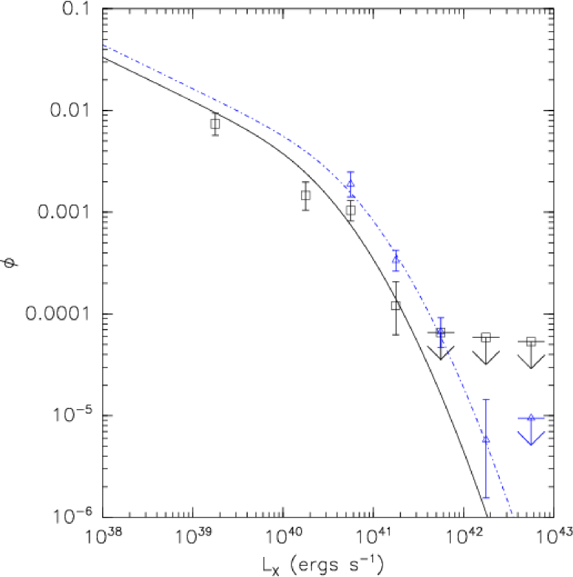
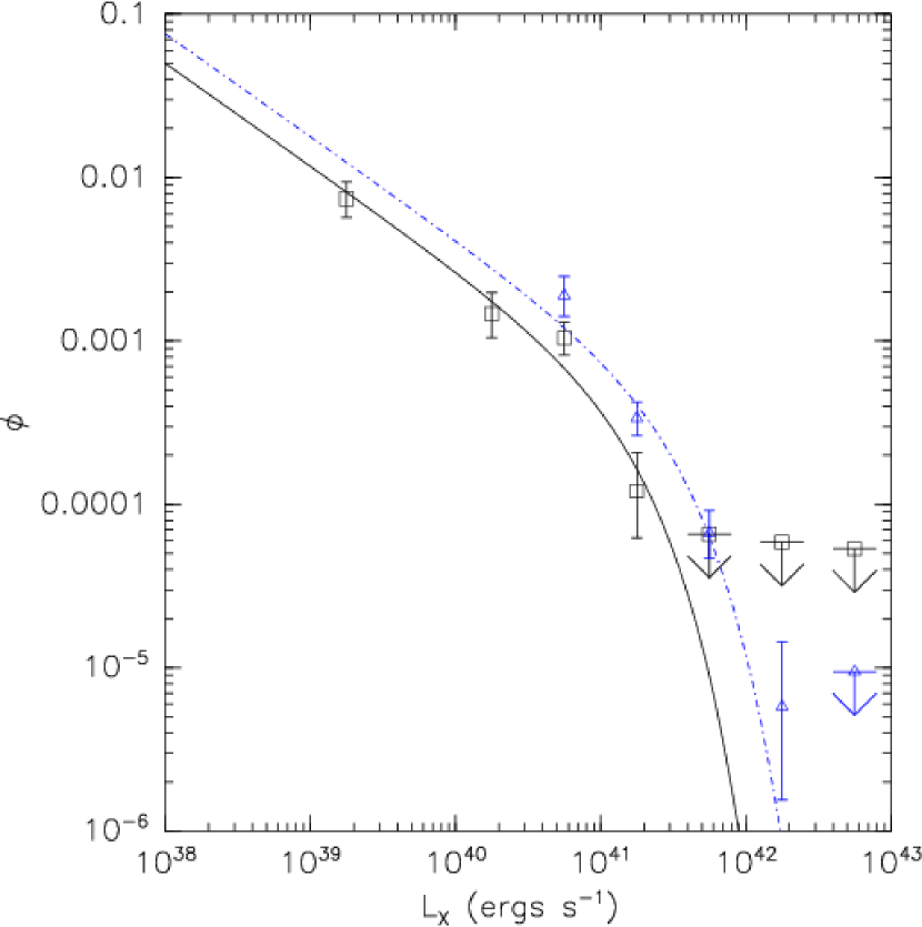
Figure 23.— Joint fits to the low-z and high-z XLFs for the full (early + late-type) galaxy sample with the log-normal (left) and Schechter functions (right). In these fits the function parameters are tied between the two XLFs, and the offset in $\log L^{*}$ is introduced as an additional fit parameter (i.e., pure luminosity evolution is assumed). The low-z XLF points are marked with (black) squares and the high-z XLF points are marked with (blue) triangles. The dashed (black) lines and dot-dashed (blue) lines show the fit to the low-z and high-z XLFs.

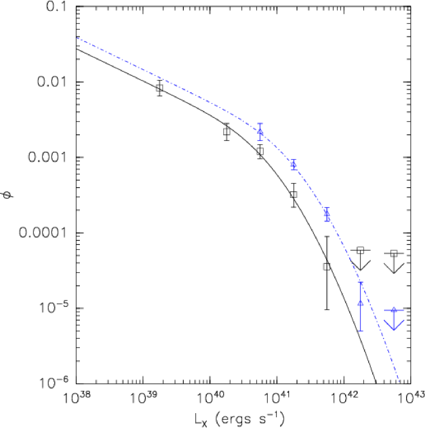
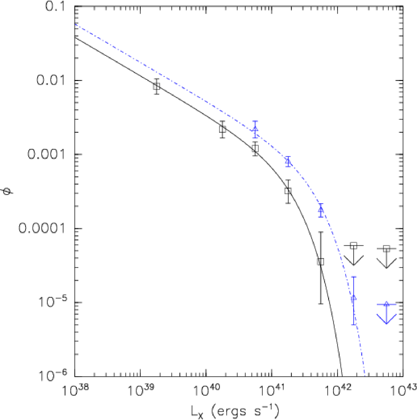
Figure 24.— As in Figure 23 for the optimistic galaxy sample.

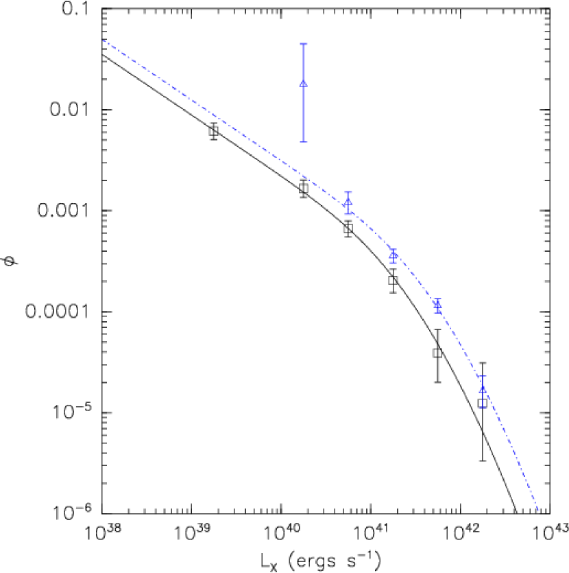
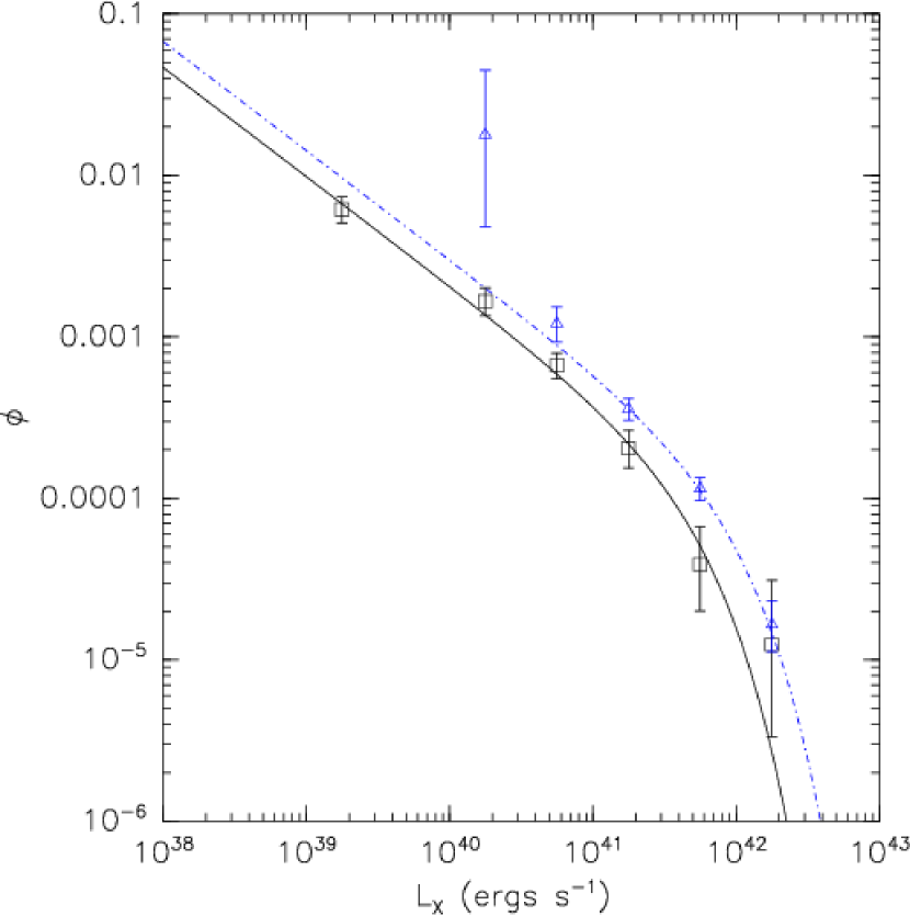
Figure 25.— As in Figure 23 for the N04 sample.

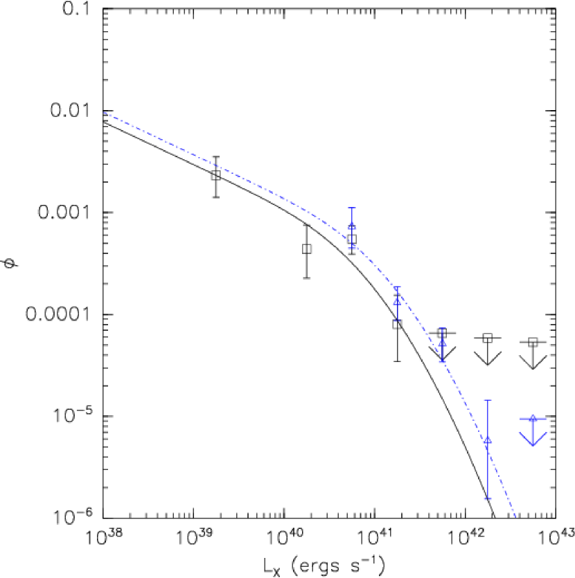
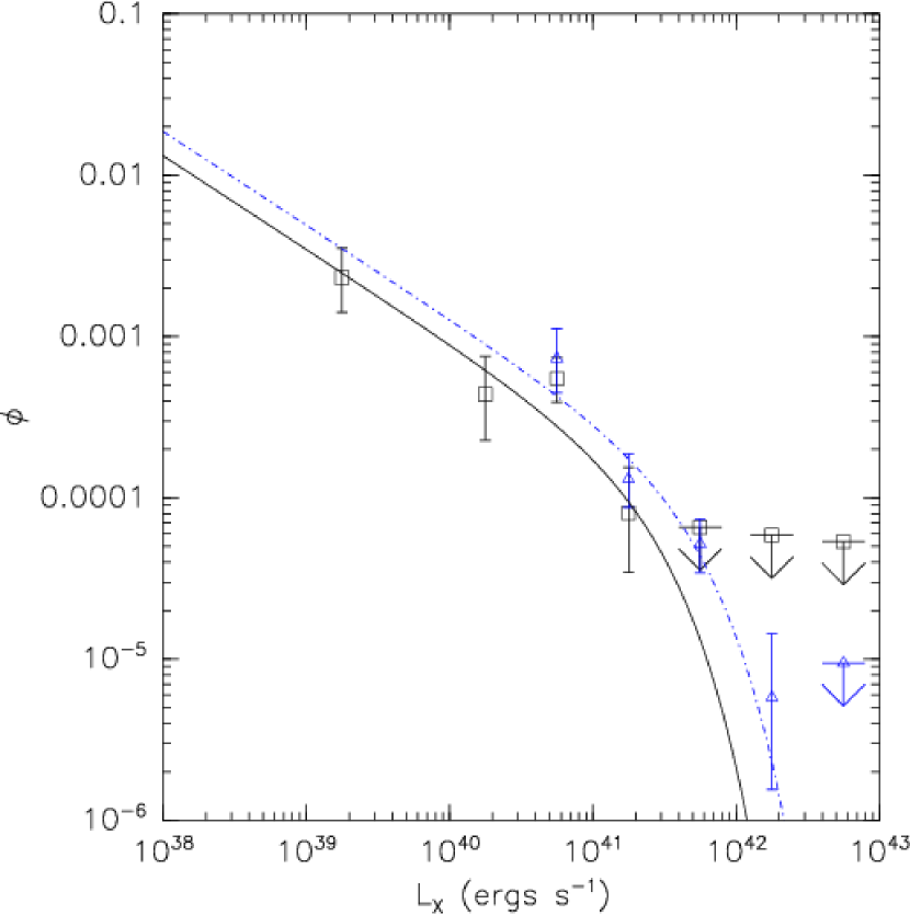
Figure 26.— As in Figure 23 for the early-type galaxy sample.

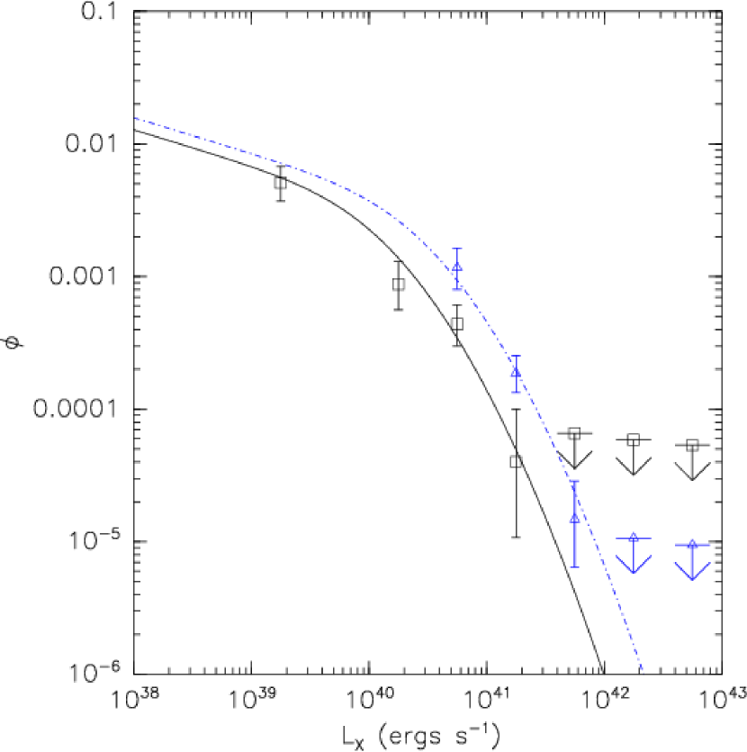
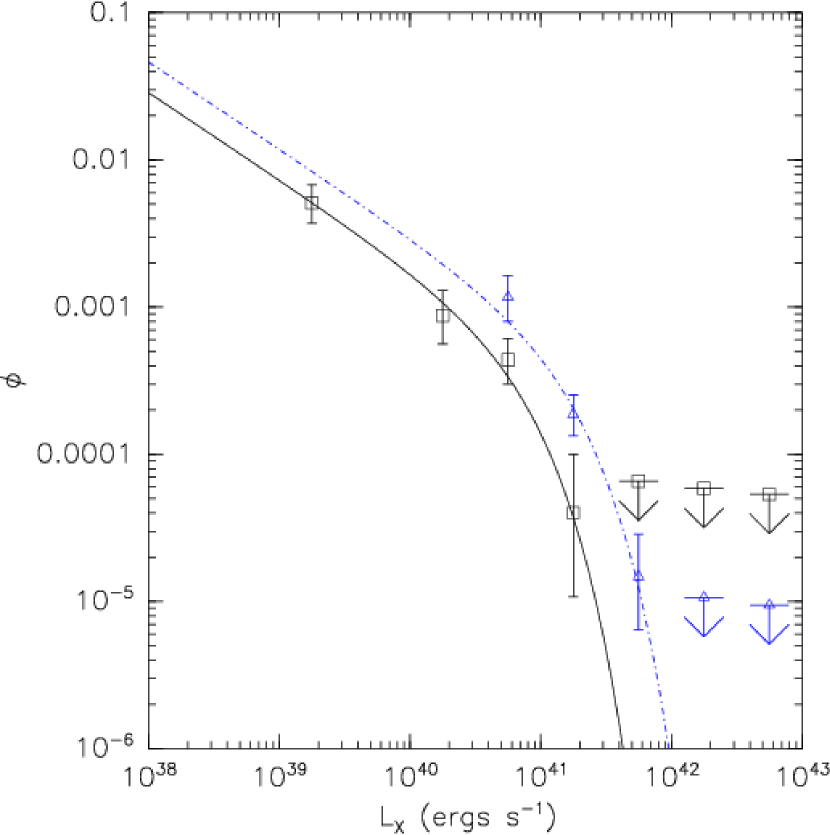
Figure 27.— As in Figure 23 for the late-type galaxy sample.

Table 6MCMC Joint Log-Normal Fits

Sample	$\log\phi^{*}$	$\log L^{*}$	$\alpha$	$\sigma$	$\Delta\log L^{*}$	$\Delta\log\rho$	$\chi^{2}/dof$	$p_{\chi^{2}}$
All galaxies	$-2.23^{+0.16}_{-0.29}$	$39.74^{+0.48}_{-0.42}$	$1.43^{+0.16}_{-0.30}$‡	$0.72^{+0.07}_{-0.07}$‡	$0.28^{+0.09}_{-0.09}$	$0.29^{+0.09}_{-0.11}$	8.2/3	95.7%
All galaxies (optimistic)	$-2.47^{+0.29}_{-0.13}$	$40.14^{+0.30}_{-0.42}$	$1.43^{+0.13}_{-0.19}$‡	$0.69^{+0.08}_{-0.06}$†	$0.35^{+0.08}_{-0.08}$	$0.35^{+0.08}_{-0.08}$	2.6/4	38.0%
Norman et al. (2004)	$-2.96^{+0.29}_{-0.24}$	$40.52^{+0.32}_{-0.35}$	$1.60^{+0.10}_{-0.10}$	$0.74^{+0.08}_{-0.07}$†	$0.25^{+0.08}_{-0.06}$	$0.27^{+0.07}_{-0.09}$	2.4/6	12.2%
Early-type galaxies	$-2.98^{+0.31}_{-0.28}$	$40.08^{+0.53}_{-0.52}$	$1.42^{+0.21}_{-0.27}$‡	$0.73^{+0.07}_{-0.07}$†	$0.23^{+0.15}_{-0.16}$	$0.23^{+0.15}_{-0.18}$	5.0/3	82.7%
Late-type galaxies	$-2.28^{+0.18}_{-0.29}$	$39.43^{+0.50}_{-0.47}$	$1.27^{+0.34}_{-0.25}$‡	$0.69^{+0.08}_{-0.06}$†	$0.34^{+0.12}_{-0.11}$	$0.33^{+0.14}_{-0.11}$	3.4/2	81.4%

Note. — Best-fitting parameters from fitting a Log-Normal function jointly to the low and high-z XLFs, allowing only $\log L^{*}$ to vary (i.e., assuming PLE).

^† Parameter is tightly constrained by prior

^‡ Parameter is moderately constrained by prior

Luminosities are in ergs s^-1 in the 0.5-2.0 keV bandpass.

$\rho$ is in ergs s^-1 Mpc^-3 in the 0.5-2.0 keV bandpass.

$p_{\chi^{2}}$ gives the $\chi^{2}$ probability at which the model fit can be rejected (note that $\chi^{2}$ is computed excluding upper limits).

Table 7MCMC Joint Schechter Fits

Sample	$\log\phi^{*}$	$\log L^{*}$	$\alpha$	$\Delta\log L^{*}$	$\Delta\log\rho$	$\chi^{2}/dof$	$p_{\chi^{2}}$
All galaxies	$-3.70^{+0.19}_{-0.22}$	$41.24^{+0.19}_{-0.14}$	$-1.63^{+0.10}_{-0.09}$	$0.29^{+0.11}_{-0.09}$	$0.30^{+0.10}_{-0.11}$	6.3/4	82.0%
All galaxies (optimistic)	$-3.50^{+0.12}_{-0.17}$	$41.32^{+0.14}_{-0.10}$	$-1.52^{+0.07}_{-0.09}$	$0.35^{+0.07}_{-0.09}$	$0.34^{+0.08}_{-0.09}$	1.0/5	4.1%
Norman et al. (2004)	$-4.23^{+0.17}_{-0.15}$	$41.75^{+0.16}_{-0.11}$	$-1.68^{+0.06}_{-0.06}$	$0.24^{+0.07}_{-0.08}$	$0.23^{+0.08}_{-0.08}$	4.1/7	23.4%
Early-type galaxies	$-4.26^{+0.30}_{-0.31}$	$41.47^{+0.34}_{-0.23}$	$-1.58^{+0.14}_{-0.13}$	$0.26^{+0.17}_{-0.18}$	$0.24^{+0.19}_{-0.18}$	5.0/4	70.8%
Late-type galaxies	$-3.62^{+0.28}_{-0.24}$	$40.91^{+0.20}_{-0.17}$	$-1.59^{+0.16}_{-0.13}$	$0.35^{+0.11}_{-0.12}$	$0.35^{+0.11}_{-0.14}$	1.6/3	35.0%

Note. — Best-fitting parameters from fitting a Schechter function jointly to the low and high-z XLFs, allowing only $\log L^{*}$ to vary (i.e., assuming PLE).

Luminosities are in ergs s^-1 in the 0.5-2.0 keV bandpass.

$\rho$ is in ergs s^-1 Mpc^-3 in the 0.5-2.0 keV bandpass.

$p_{\chi^{2}}$ gives the $\chi^{2}$ probability at which the model fit can be rejected (note that $\chi^{2}$ is computed excluding upper limits).

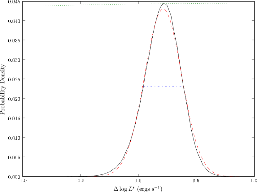
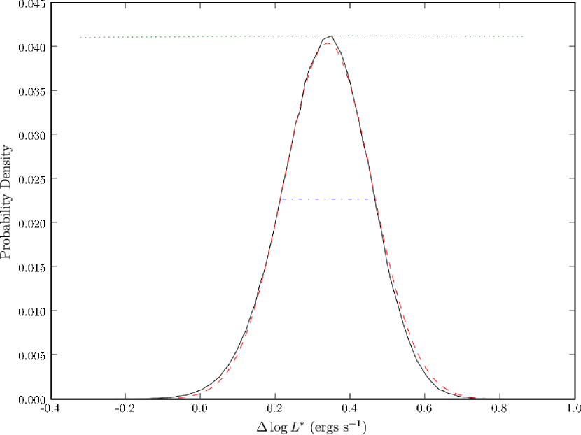
Figure 28.— The posterior probability distributions for $\Delta\log L^{*}$ for the early-type (left) and late-type (right) galaxy samples based on log-normal fits (very similar results were obtained from the Schechter function fits). The solid solid (black) lines show the posterior probability, the dashed (red) lines shows a Gaussian distribution with the same mean and standard deviation as the posterior, the dotted (green) line show the prior, and the dot-dashed line shows the 68% confidence interval.

4. Discussion

We used the GOODS survey to derive X-ray luminosity functions for sources segregated by optical/NIR spectral type. We split the sources into low ($z<0.5$) and high ($0.5<z<1.2$) redshift samples in order to investigate evolution. We also explored an “optimistic” sample (when our galaxy selection criterion is relaxed) and the N04 XLFs for comparison. We implemented MCMC techniques for linear, log-normal and Schechter function fits to the binned XLFs. This has given us a reliable statistical assessment of the XLFs and any evolution. While in general either a log-normal or Schechter function could fit a given XLF well, this is due in part to the relatively sparse sampling in the XLFs presented here. Better data would be required to constrain the shapes of the XLFs. A consequence of this is that the faint-end slopes of the XLFs are somewhat uncertain, with the log-normal and Schechter function fits giving divergent predictions for the numbers of galaxies expected in deeper exposures.

4.1. Comparison with Local XLFs for Different Spectral Types

We showed that the difference in the early and late-type galaxy XLFs was only significant at the $\sim 90\%$ and $\sim 97\%$ level for the z$\sim 0.25$ and $z\sim 0.75$ XLFs. This is suggestive that there is a difference between the spectral type-selected XLFs at each redshift but clearly better data will be required to strengthen this result. Early and late-type XLFs were also derived in Georgantopoulos et al. (2005, hereafter G05) for a sample of galaxies at z$<0.2$. In Figure 29 we plot our low-z early and late-type normal/starburst sample XLFs with the G05 XLFs also shown. There is good overall agreement between the two sets of XLFs, with the exception of the G05 early-type point at $L_{X}\sim 10^{39}\ \rm ergs\ s^{-1}$ being marginally higher than our corresponding point. The mean redshift of our low-z galaxy XLFs is $\sim 0.3$ for both the early-type and late-type samples, tentatively implying that there has been little or no evolution between z $\sim 0.1$ and z $\sim 0.3$. However, $\sim 40\%$ of the G05 galaxy sample was comprised of CDF sources, most of which probably are also in our normal/starburst galaxy sample. Having overlapping sources between our GOODS and the G05 samples would obviously dilute any difference between the XLFs.

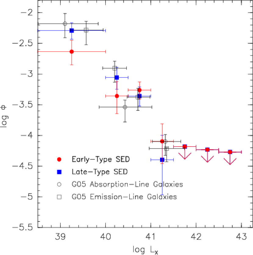
Figure 29.— The low-z spectral type and galaxy selected XLFs from this work shown along with the XLFs from G05.

4.2. Evolution

In all of the samples discussed here the low-z and high-z XLFs differ at a confidence of $>99\%$, showing there is statistically-significant evolution with redshift. When log-normal and Schechter functions are fit to the individual XLFs, not surprisingly the resulting $\phi^{*}$ and $L^{*}$ values differ for a given sample, however the implied luminosity densities $\rho$ do not in general differ significantly. In other words, our computed values of $\rho$ are insensitive to whether the log-normal or Schechter functions are used, giving additional confidence in the resulting values. We also fit the low and high redshift XLFs simultaneously with the log-normal and Schechter functions, with the main function parameters (i.e., $\log\phi^{*}$, $\log L^{*}$ and the slopes) tied between the two XLFs but assuming pure luminosity evolution by fitting also for $\Delta\log L^{*}$. The results for $\Delta\log L^{*}$ also do not depend strongly on whether the log-normal or Schechter functions are used. The corresponding $\Delta\log\rho$ values were nearly identical to the $\Delta\log L^{*}$ values, which might be expected since $\log\rho$ depends linearly on $\log L^{*}$ when all other parameters are fixed (and the differences observed between $\Delta\log L^{*}$ and $\Delta\log\rho$ show the impact of jointly varying $\log\phi^{*}$ and the slopes).

The early and late-type galaxy $\Delta\log L^{*}$ values were 0.23 and 0.34 (from the log-normal fits), showing stronger evolution for late-type galaxies. This corresponds to early and late-type galaxies being factors of $\sim 1.7$ and $\sim 2.2$ brighter, respectively, between $z\sim 0.25$ and $z\sim 0.75$. It is not clear whether the evolution observed in early-type galaxies is due to passive evolution of the low-mass X-ray binary population (Ghosh & White, 2001; Ptak et al., 2001) or is due to enhanced star formation as expected in the case of late-type galaxies. However we note that our galaxy type selection is based on galaxy SED type rather than morphological type, and therefore these galaxies have red colors. This suggests that they are not actively star forming. The lack of any redshift dependence in the $F_{X}$/NIR flux ratio (see Appendix C) may be constraining to LMXRB evolution models since LMXRB do not “turn on” instantenously as discussed in Ghosh & White (2001), however the scatter here is large.

Pure luminosity evolution is often expressed as $L^{*}(z)=(1+z)^{p}L^{*}(z=0)$. With that parametrization and $\Delta\log L^{*}$ being measured between two redshifts $z_{1}$ and $z_{2}$, $p=\frac{\Delta\log L^{*}}{\log(1+z_{2})-\log(1+z_{1})}$ or $p\sim 6.8\Delta\log L^{*}$ for $z_{1}\sim 0.25$ and $z_{2}\sim 0.75$. The $\Delta\log L^{*}$ values then correspond to $p_{\rm early}=1.57^{+1.09}_{-1.03}$ and $p_{\rm late}=2.33^{+0.75}_{-0.82}$. The late-type galaxy evolution is consistent with the FIR evolution of $p\sim 3$. Also note that Georgakakis et al. (2007) similarly found $p\sim 2.4$ for star-forming galaxies from the GOODS-N, using methods somewhat independent of those discussed here (although in both studies low $L_{X}$, X-ray hardness, and X-ray/optical flux ratio were among the selection criteria). The full sample $\Delta L^{*}$ was 0.29, not surprisingly intermediate to the early-type and late-type galaxy XLF values. The optimistic sample resulted in a $\Delta\log L^{*}$ value of 0.35, basically the same as the late-type galaxy value. However this may be somewhat coincidental since the optimistic sample is most likely also introducing low-luminosity AGN. However, any AGN activity is probably not dominating the near-IR-optical and the X-ray bandpass since otherwise the X-ray/optical ratios and/or the X-ray hardnesses would have resulted in an AGN classification (see Appendix A). Nevertheless the results of our analysis of the optimistic sample probably represents a reasonable limit to the maximum amount of evolution expected for the soft X-ray emission from normal/starburst galaxies between $z\sim 0.25$ and $z\sim 0.75$. We also note that the luminosity densities inferred for the full sample XLFs are very similar to the luminosity densities inferred for the N04 XLFs, while the optimistic sample XLFs resulting in luminosity densities $\sim 0.2$ dex higher. Better data (either from deeper Chandra exposures or future X-ray missions) would of course result in smaller errors on the X-ray properties of the sources which in turn improve the classification probabilities, as well as increasing the number of sources populating the low-luminosity end of the XLFs.

5. Summary

We have computed XLFs for normal/starburst galaxies in the GOODS for sources with X-ray counterparts, and fit the XLFs with linear models using “traditional” techniques as well as Markov-Chain Monte Carlo techniques. From the photometric redshift fitting procedure we classified 40 galaxies as early-type and 46 galaxies as late-type based on their SEDs. The early-type galaxy XLFs tend to be slightly flatter than those for late-type galaxies, although from the MCMC analysis the significance of this result is only at the $1-2\sigma$ level. The early and late-type galaxy sample XLFs at z$\sim 0.25$ are consistent with the low-redshift early and late-type XLFs of Georgantopoulos et al. (2005). We used the MCMC approach to also fit the XLFs with log-normal and Schechter functions. The XLFs discussed here all show significant evolution between $z\sim 0.25$ and $z\sim 0.75$. We jointly fit the low and high-redshift XLFs assuming pure luminosity evolution, allowing only $L^{*}$ to vary between the XLFs, which resulted in evolution of $(1+z)^{1.6}$ and $(1+z)^{2.3}$ for the early-type and late-type galaxy samples. The late-type galaxy evolution derived here is consistent with the star-forming galaxy X-ray evolution given in Georgakakis et al. (2007). Including sources with ambiguous classification results in an “optimistic” galaxy sample with a total galaxy X-ray evolution of $(1+z)^{2.4}$, essentially the same value as derived for late-type galaxies. The optimistic sample XLF evolution suggests that the maximum amount of evolution in the X-ray emission of normal/starburst galaxies at these redshifts is $(1+z)^{2.4\pm 0.5}$.

The Bayesian fitting approach here could be expanded to include additional uncertainties that might impact this analysis, such as the redshift errors (see, e.g., Dahlen et al., 2005), the uncertainties in the completeness correction and the uncertainties the X-ray and optical fluxes of the sources. A larger impact on our results would likely result from including radio and FIR data from the GOODS fields, which we will explore in future work. This will improve both the SED fitting (and hence the galaxy type determination) and give an independent star-formation rate estimation (see also Georgakakis et al., 2007). It may also be possible to simultaneously fit for the multi-variate luminosity functions and the individual galaxy types, activity types and redshifts (with any spectroscopic redshifts used as tight priors), at least in an iterative fashion (i.e., where the current luminosity function estimates guide the galaxy type and photometric redshift probabilities). Finally, advanced Bayesian model selection techiniques, as discussed in Trotta (2007) and references therein, can be applied here to guide the parameters of future observations by predicting the ability of future data to prefer a given model and arrive at a given set of constraints.

Appendix A GOODS X-ray Sample Properties and Galaxy Selection

Here we discuss our methodology for classifying the sources, and we also discuss the statistical properties of the sample. Note that the relevant point of our classification is not whether the entire SED is dominated by star-formation or an AGN, but which of these is dominating the soft X-ray band.

A.1. Bayesian Selection

N04 selected normal/starburst galaxies from the full CDF-N and CDF-S samples using a Bayesian classification procedure, where priors were constructed from the a set of galaxies with well-determined optical types, normal/starburst galaxy, type-1 AGN and type-2 AGN (hereafter galaxy, AGN1 and AGN2). The product of the prior distributions for a class and the likelihood for the observed parameters for a given source gave the probability that the source was drawn from that class. Here we follow the same procedure with several improvements. First, sources with small differences between the probabilities in each class should have been considered uncertain since these conditions occur when the separation of the sources parameter values and the parent distribution means are small relative to the parameter errors. Here we use the Bayesian “odds ratio”, or the ratio of posterior probabilities for the classes being compared. In Bayesian model testing a model is considered to be favored only when the odds ratio exceeds at least 3 (while odds ratios greater than 10 are preferred). Second, the parameter likelihoods were handled somewhat simplistically, with Gaussian errors assumed on each parameter and a constant error in $\log L_{X}$ and $\log L_{X}-\log L_{opt}$ of 0.25. The Gaussian assumption is not correct for hardness ratio errors and $\log L_{X}$ errors when the number of counts detected for the source is small. However, it turns out that the Gaussian approximation to hardness ratio errors is conservative (Park et al., 2006). Here we use the larger of the asymmetric errors on count rate given in Alexander et al. (2003). We assume that $\Delta F_{X}/F_{X}=\Delta C/C$ where $\Delta F_{X}$ is the error on X-ray flux and $\Delta C$ is the error on X-ray count rate C given in Alexander et al. We then take the error on $\log L_{X}$ to be given by $\frac{\Delta L_{X}}{L_{X}\log(10)}$ where $\Delta L_{X}=L_{X}\frac{\Delta F_{X}}{F_{X}}$. This is valid only when $\Delta F_{X}/F_{X}\ll 1$, however this is the case for the majority of the X-ray sources. Finally, N04 did not account for k-corrections in the optical data when computing X-ray/optical flux ratios (k-corrections to the X-ray data were not necessary since an energy index of 1.0 was assumed for every source). As discussed below, k-corrections are now included in the computation of the priors and in the galaxy classification.

A.2. Priors

Szokoly et al. (2004) reported classifications based on the optical spectra alone, in the classes “ABS” (no or only absorption lines are present in the spectrum), “LEX” (a low-ionization emission line spectrum), “HEX” (a high-ionization emission line spectrum), and “BLAGN” (broad emission lines are found). All of the BLAGN sources should correspond to AGN1 sources, by definition, however a broad line AGN may be present in the other classes where there was not sufficient signal to detect a broad-line component. The HEX and LEX classes should be dominated by type-2 AGN and star-forming galaxies, respectively. However the LEX classification includes some AGN where low signal-to-noise or dilution of the nuclear spectrum due to aperture effects (Moran et al., 2002) has precluded the detection of high-excitation emission lines. For several LEX sources the statistics are sufficient for an AGN component to be identified from line-ratio diagnostics. We therefore derive priors using only ABS sources as galaxies, HEX sources and LEX sources with AGN line ratios as AGN2, and BLAGN sources as AGN1. We required that the X-ray sources have a corresponding entry in the Alexander et al. catalog since that catalog is used for the X-ray properties of the GOODS sample.

We initial only selected sources with z $<=$1.2 however this resulted in only 8 AGN2 sources. Since AGN2 are known to have flat X-ray spectra, and hence a minimal k-correction, we relaxed the redshift constraint to z $<=$ 2 for that class. The final tally was then 11 AGN2 sources, 11 AGN1 sources and 15 (normal/starburst) galaxy sources. The mean offsets between the R and K band magnitudes reported in Szokoly et al. and the R and $\rm K_{s}$ bands used in the GOODS survey were computed in order to adopt the priors based on the Szokoly et al. source for use with GOODS data. This was done regardless of spectral type and we found offsets of 0.22 magnitudes in R and 1.9 magnitudes in K, with a standard deviations of 0.16 and 0.21 magnitudes.

As shown in Figure 3, k-corrections to the X-ray/R and X-ray/K band flux ratios can be significant. Since only K and R band magnitudes are listed in Szokoly et al., we cannot apply the same interpolation procedure for k-corrections as was done with GOODS data. However, we can use the R-K color to estimate the spectral type of the source, and apply a mean k-correction based on that type. We show in Figure 30 the R-$\rm K_{s}$ colors for the full sample, with early-type, late-type and irregular/starburst galaxies marked separately. While there is some overlap, we manually selected linear functions to delineate the spectral type as a function of redshift, as shown in the figure. The early/late-type galaxy separation is given by R-$\rm K_{s}$ = 1.0 + 2.2z and the late-type/starburst galaxy separation is given by R-$\rm K_{s}$ = 0.2+2.0z.

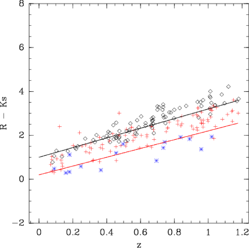
Figure 30.— R-$\rm K_{s}$ color plotted as a function of redshift for the early-type, late-type and irregular/starburst galaxies in the full sample. Also plotted are the lines used to separate these spectral types in the computation of priors in the Szokoly sample.

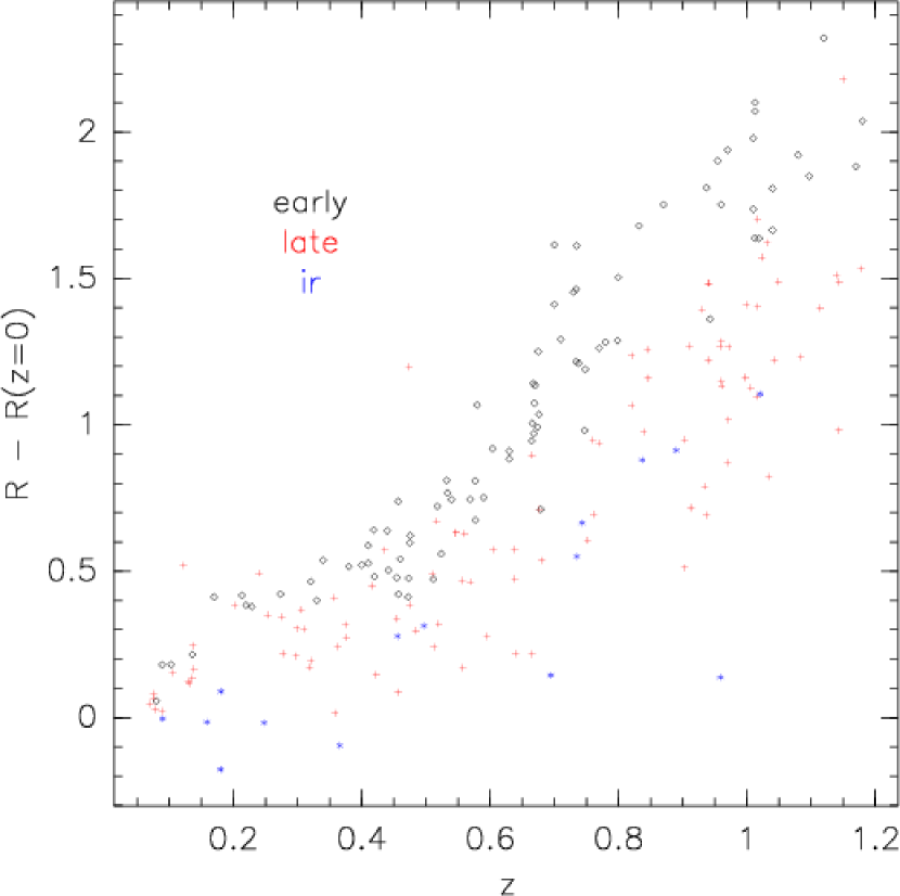
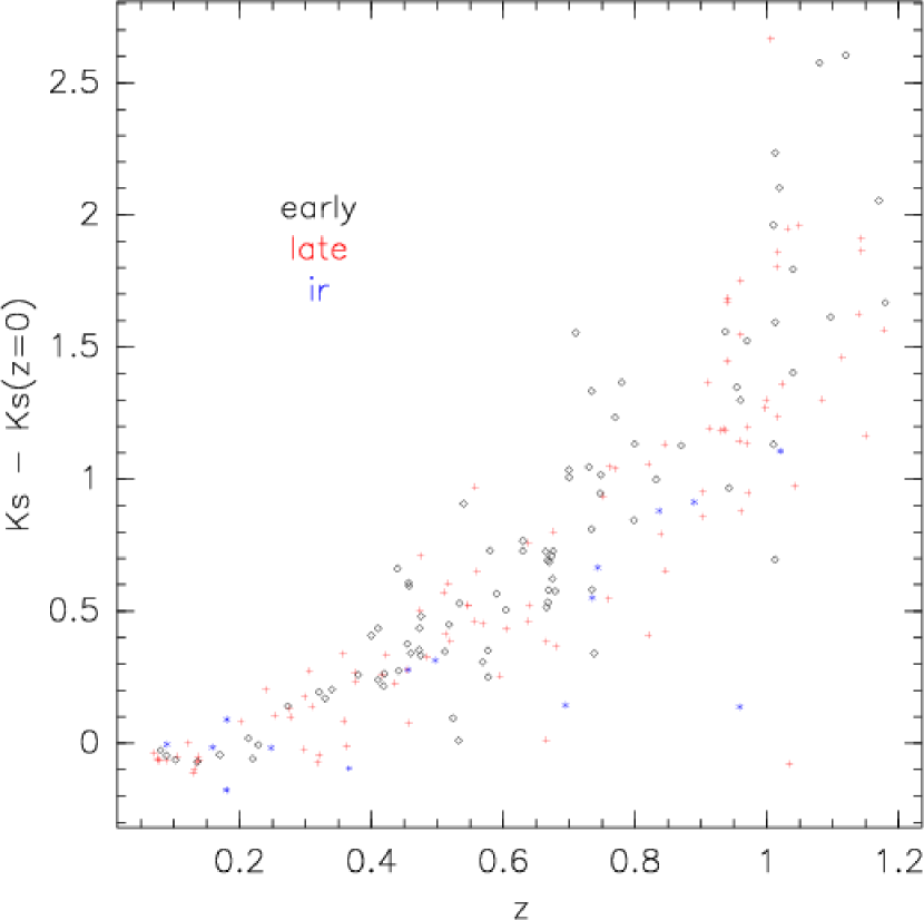
Figure 31.— K-corrections plotted as a function of redshift for R-band (left) and $\rm K_{s}$-band (right) magnitudes. The quantity plotted is the difference between the observed and k-corrected magnitude. Early-type galaxies are plotted with diamonds , late-type galaxies are plotted with pluses, and irregular/starbursts are plotted with asterisks.

Having established a crude spectral type color selection, we proceeded by plotting the R and $\rm K_{s}$ k-corrections as a function of redshift for each spectral type, shown in Figure 31. For each spectral type we determined the k-correction/redshift correlation. Again, while the dispersion in k-correction is large, this resulted in at least an approximate k-correction that was applied to the sources when computing the priors.

We list in Table 8 the mean and standard deviation for the parameters $L_{X}$, $HR$ (X-ray hardness), X-ray/R-band flux ratio and X-ray/$\rm K_{s}$-band flux ratio computed using the prior samples. The priors were then modeled as Gaussians with these values for the Gaussian mean and standard deviation, as discussed in N04 The full sample is listed in Tables 11 and 12, where we list the final classification along with the Bayesian odds ratios for the models. For example, if the preferred class for a source is “galaxy”, then the odds ratios are given for galaxy vs. AGN1 and galaxy vs. AGN2. For comparison, 30/43 of the OBXF sources from Hornschemeier et al. (2003) are in our GOODS-N sample, and all but one were classified as (normal/starburst) galaxies. The remaining source (XID=458) had “galaxy” as the highest probability, but only at a factor of 2.1 higher than the AGN2 probability and hence is only in the “optimistic” sample. A spectral type was given for 28 of the 30 OBXF sources with matches, which is also listed in Table 11. Overall there was good agreement between our SED types and the spectral types, with 7/9 of the absorption-line galaxies having an early-type SED classification and 15/17 emission-line galaxies having a late-type SED classification (the remaining 2 sources were “composite” galaxies having both absorption and emission lines). Similarly we also list the redshift found in Georgakakis et al. (2007), if present, for the GOODS-N sources, where it can be seen there is good overall agreement between the redshifts.

Table 8Bayesian Prior Parameters

Class	Parameter	Mean	$\sigma$
Normal/Starburst Galaxies	HR	-0.19	0.46
	$\log L_{X}$	40.6	0.7
	$\log F_{X}/F_{opt}$	-3.2	0.7
	$\log F_{X}/F_{K}$	-3.4	0.7
AGN2	HR	0.16	0.37
	$\log L_{X}$	41.1	1.1
	$\log F_{X}/F_{opt}$	-2.2	1.0
	$\log F_{X}/F_{K}$	-2.7	0.7
AGN1	HR	-0.51	0.05
	$\log L_{X}$	42.9	0.4
	$\log F_{X}/F_{opt}$	-1.2	0.4
	$\log F_{X}/F_{K}$	-1.4	0.5

Appendix B Statistical Properties of the Samples

In Figure 32 we show histograms of the photon indices, binned separately by spectral type. The photon index distributions are similar, peaking at $\Gamma\sim 1.2-1.4$. However note this is due in part to the adoption of $\Gamma=1.4$ in Alexander et al. for sources with low signal-to-noise. The number of irregular/starburst sources is very low and is likely to be similar to the rest of the sample. We list in Table 9 the number of sources in each sample (i.e., divided by field, host galaxy type and bandpass) along with the mean, standard deviation, minimum and maximum (k-corrected) magnitude. We also give the similar statistics for $\log F_{X}$ and $\log L_{X}$. Note that $\rm K_{s}$ magnitudes were not always available. An immediate conclusion is that the AGN contribution is most significant for the irregular/starburst samples since the mean X-ray luminosities are $\sim 10^{42}\rm\ ergs^{-1}$, the luminosity at which AGN emission starts to dominate the X-ray band. The corresponding values after galaxy selection are listed in Table 10.

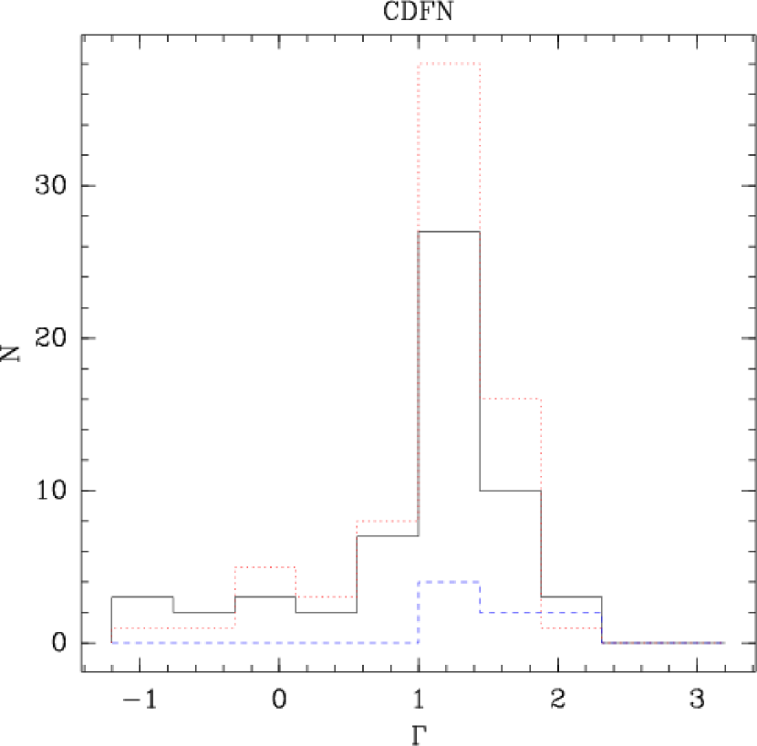
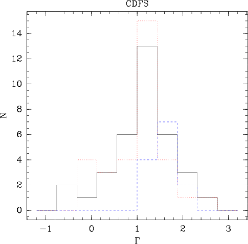
Figure 32.— Distribution of photon indices for the CDF-N (left) and CDF-S (right) sources, binned by galaxy spectral type (black, solid line=early-type, red, dotted line=late-type, blue, dashed line=starburst/irregular).

Table 9X-ray and Optical Statistical Properties

Field	Band	SED Type	N	Mean	$\sigma$	Min.	Max.
CDFN	B	early	57	22.26	1.07	19.13	24.27
CDFN	R	early	57	21.29	1.16	18.03	23.45
CDFN	Ks	early	57	18.90	0.94	17.09	21.32
CDFN	J	early	57	20.32	1.02	17.45	22.32
CDFN	logFX	early	57	-16.16	0.48	-17.38	-14.64
CDFN	logLX	early	57	40.96	0.70	38.91	42.42
CDFN	B	late	73	21.94	1.16	19.64	24.66
CDFN	R	late	73	21.20	1.15	18.59	23.81
CDFN	Ks	late	73	19.18	0.85	17.62	21.69
CDFN	J	late	73	20.41	0.95	18.09	22.53
CDFN	logFX	late	73	-16.03	0.79	-17.39	-13.64
CDFN	logLX	late	73	41.01	1.03	38.89	43.33
CDFN	B	ir	8	22.11	1.48	19.91	24.54
CDFN	R	ir	8	21.73	1.38	19.84	23.88
CDFN	Ks	ir	8	20.20	1.55	18.27	22.47
CDFN	J	ir	8	21.18	1.39	19.69	23.13
CDFN	logFX	ir	8	-15.27	1.27	-16.74	-13.81
CDFN	logLX	ir	8	41.73	1.52	39.72	43.54
CDFS	B	early	36	21.62	1.48	18.11	25.95
CDFS	R	early	36	20.54	2.08	16.25	27.61
CDFS	Ks	early	29	18.73	1.22	16.07	21.59
CDFS	J	early	29	19.86	1.38	16.27	22.80
CDFS	logFX	early	36	-15.80	0.56	-16.88	-14.51
CDFS	logLX	early	36	41.32	0.65	39.65	42.77
CDFS	B	late	32	22.03	1.68	17.34	25.95
CDFS	R	late	32	21.08	1.70	16.71	24.97
CDFS	Ks	late	26	19.08	1.27	15.94	21.82
CDFS	J	late	26	20.25	1.50	16.03	22.39
CDFS	logFX	late	32	-15.83	0.63	-16.74	-14.39
CDFS	logLX	late	32	41.31	0.83	39.91	42.90
CDFS	B	ir	13	21.45	1.55	19.24	24.65
CDFS	R	ir	13	21.00	1.69	18.00	24.30
CDFS	Ks	ir	7	20.76	1.33	19.58	22.89
CDFS	J	ir	7	21.45	1.30	19.98	23.64
CDFS	logFX	ir	13	-14.90	1.13	-16.27	-13.36
CDFS	logLX	ir	13	41.98	1.78	39.44	44.03

Table 10X-ray and Optical Statistical Properties , Galaxies only

Field	Band	SED Type	N	Mean	$\sigma$	Min.	Max.
CDFN	B	early	27	21.54	0.91	19.13	22.91
CDFN	R	early	27	20.50	1.00	18.03	21.88
CDFN	Ks	early	27	18.31	0.61	17.09	19.56
CDFN	J	early	27	19.60	0.81	17.45	20.75
CDFN	logFX	early	27	-16.32	0.31	-16.93	-15.60
CDFN	logLX	early	27	40.63	0.66	38.91	41.47
CDFN	B	late	36	21.45	1.01	19.64	23.65
CDFN	R	late	36	20.73	1.04	18.59	22.87
CDFN	Ks	late	36	18.95	0.66	17.78	20.59
CDFN	J	late	36	20.02	0.80	18.09	21.45
CDFN	logFX	late	36	-16.39	0.32	-17.12	-15.72
CDFN	logLX	late	36	40.41	0.64	38.89	41.41
CDFN	logFX	ir	1
CDFN	logLX	ir	1
CDFS	B	early	13	20.47	1.01	18.11	21.52
CDFS	R	early	13	19.15	1.38	16.25	20.96
CDFS	Ks	early	11	17.63	0.76	16.07	18.74
CDFS	J	early	11	18.58	1.07	16.27	20.09
CDFS	logFX	early	13	-15.97	0.46	-16.59	-15.18
CDFS	logLX	early	13	40.92	0.62	39.65	41.85
CDFS	B	late	10	20.52	1.61	17.34	21.83
CDFS	R	late	10	19.70	1.58	16.71	21.23
CDFS	Ks	late	9	18.08	1.21	15.94	19.54
CDFS	J	late	9	18.92	1.56	16.03	20.11
CDFS	logFX	late	10	-15.94	0.43	-16.36	-15.07
CDFS	logLX	late	10	40.62	0.49	39.91	41.43
CDFS	B	ir	2	21.03	0.79	20.47	21.59
CDFS	R	ir	2	20.63	0.74	20.11	21.15
CDFS	Ks	ir	2	19.66	0.11	19.58	19.74
CDFS	J	ir	2	20.32	0.48	19.98	20.66
CDFS	logFX	ir	2	-16.24	0.05	-16.27	-16.20
CDFS	logLX	ir	2	40.35	0.48	40.01	40.69

Appendix C X-ray Flux Ratios

Since X-ray/R-band and X-ray/$\rm K_{s}$-band flux ratios are used in selection criteria for this paper, we discuss here the potential impact of any luminosity or redshift dependence of these quantities. In Figures 33 and 34 we plot the X-ray/R-band and X-ray/$\rm K_{s}$-band flux ratios as a function of luminosity, before and after applying k-corrections. Figures 35 and 36 show the flux ratios plotted as a function of redshift. In the luminosity versus flux ratio plots we show the regions resulting from our Bayesian prior analysis. These ellipses show the 1 and 2$\sigma$ regions where the $\sigma$ value is based on the standard deviation of the parent populations. In other words, the width and height of the 1$\sigma$ regions are the standard deviations of the X-ray luminosity and given flux ratio for the corresponding class (galaxy, AGN1 or AGN2), and correspond to the 68% and 95% probability intervals for that parameter. However, this assumes that the X-ray luminosity and flux ratios are not correlated, and since this is not the case, these regions should not be interpreted as joint confidence regions. The intention here is to simply show the regions in the $\log L_{X}-\log F_{X}/F_{R}$ and $\log L_{X}-\log F_{X}/F_{K_{s}}$ planes from which our normal/starburst samples are being selected.

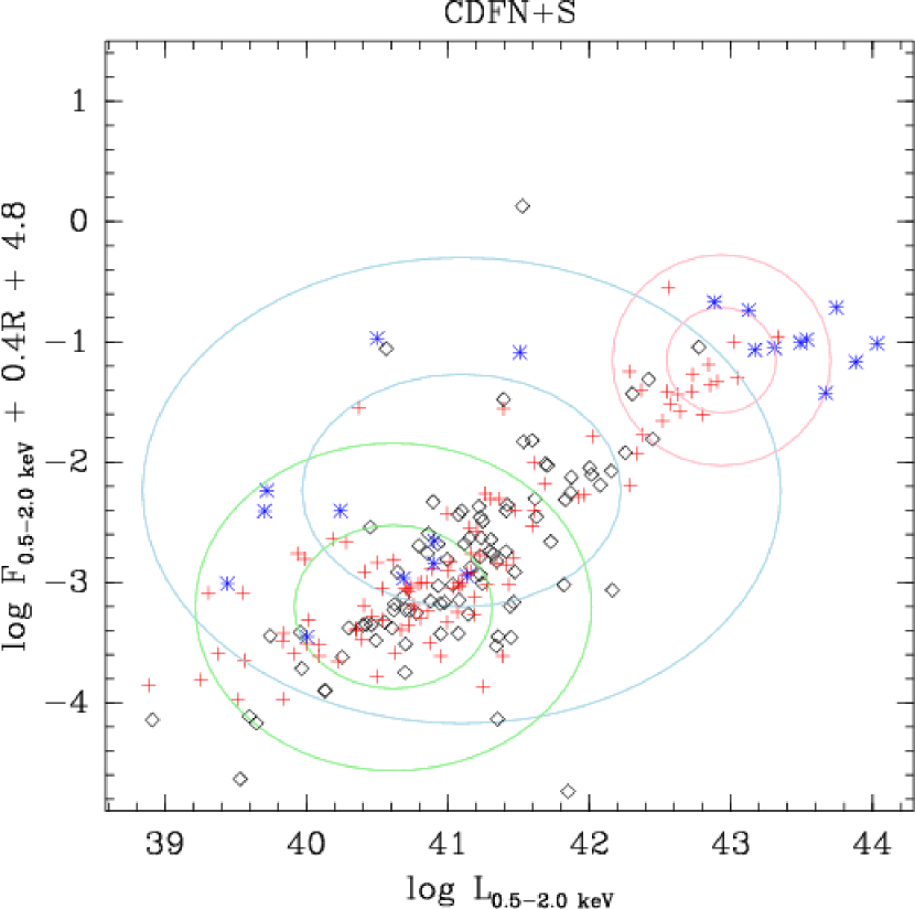
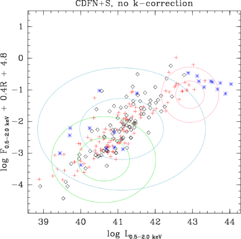
Figure 33.— The X-ray/R-band flux ratio plotted as a function of X-ray luminosity, including (left) and not including (right) k-corrections. Early-type, late-type and irregular/starburst SED sources are marked with (black) diamonds, (red) pluses, and (blue) asterisks, respectively. The ellipses show the 1 and 2$\sigma$ intervals computed for the prior probability distributions for galaxies, AGN1 and AGN2 for $\log L_{X}$ and $\log F_{X}/F_{R}$. Note that these intervals correspond to standard deviations computed separately for these parameters (i.e., the widths of the ellipses give the 68% and 95% probability intervals for $\log L_{X}$ for each type), which assumes no correlation between $L_{X}$ and $F_{X}/F_{R}$.

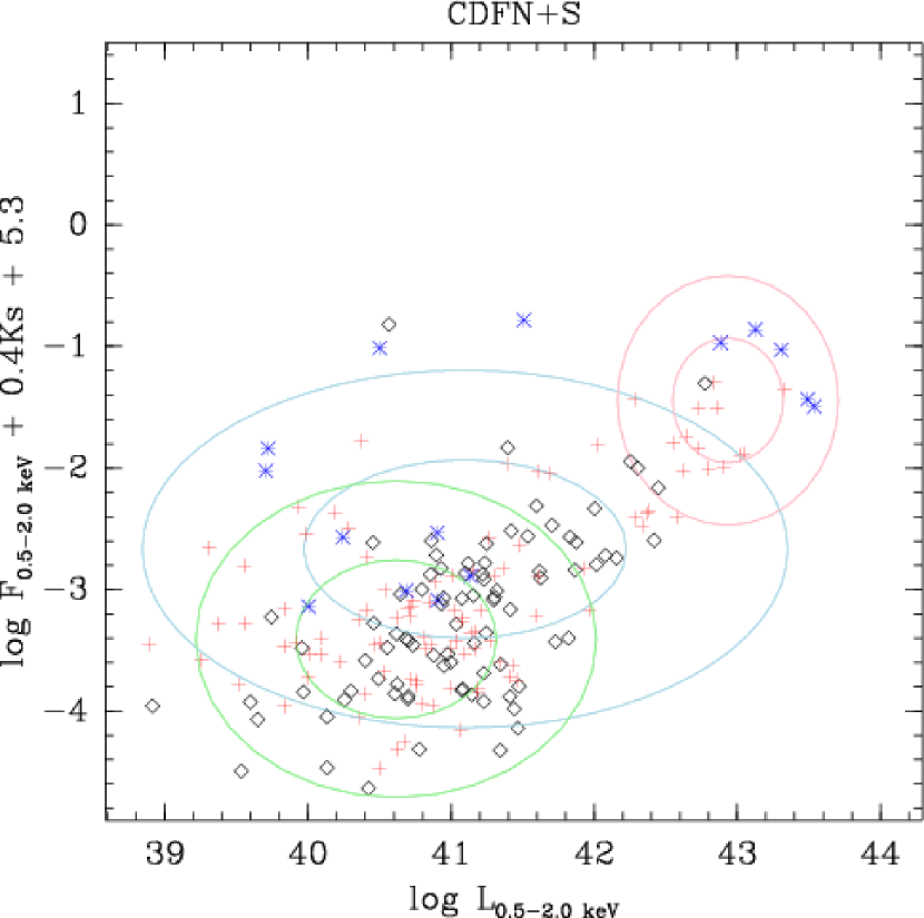
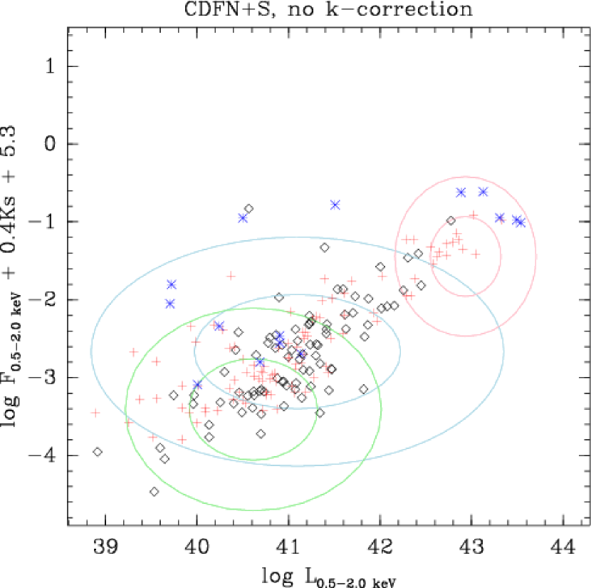
Figure 34.— The X-ray/$\rm K_{s}$-band flux ratio plotted as a function of X-ray luminosity, including (left) and not including (right) k-corrections. Symbols and ellipses are as in Figure 33.

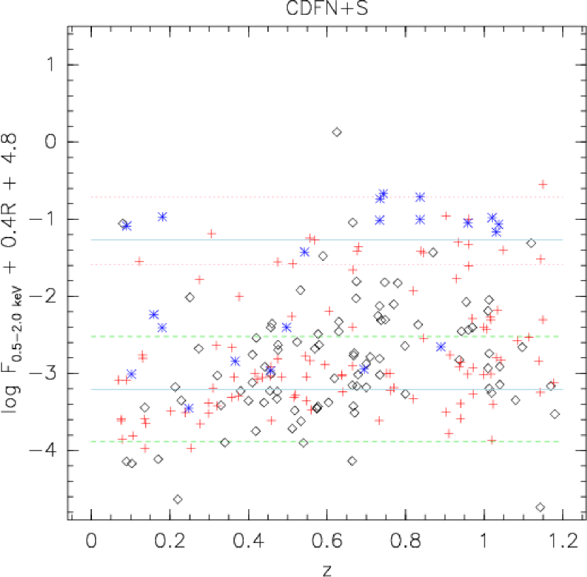
Figure 35.— The X-ray/R-band flux ratio plotted as a function of redshift, including (left) and not including (right) k-corrections. Early-type, late-type and irregular/starburst SED sources are marked with (black) diamonds, (red) pluses, and (blue) asterisks, respectively. Horizontal lines are drawn showing the 1$\sigma$ probability intervals for the flux ratio for galaxies (green dashed lines), AGN1 (red dotted lines) and AGN2 (blue solid lines).

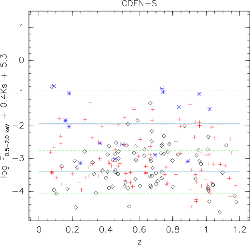
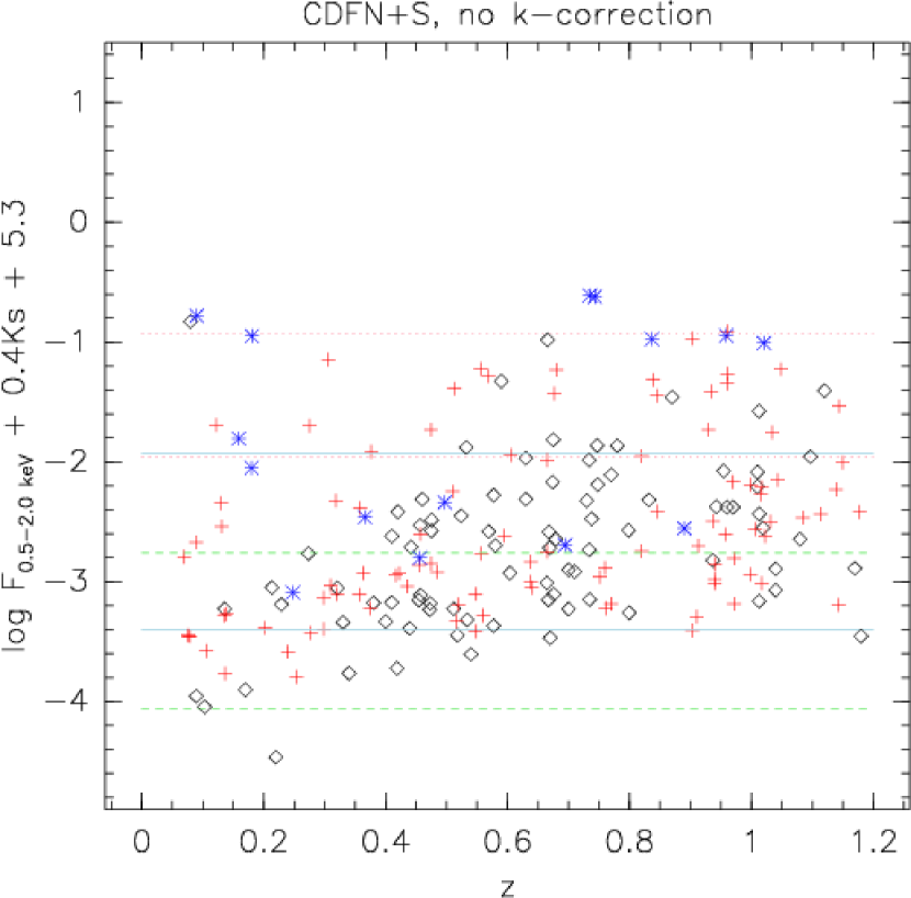
Figure 36.— The X-ray/$\rm K_{s}$-band flux ratio plotted as a function of redshift, including (left) and not including (right) k-corrections. Early-type, late-type and irregular/starburst SED sources are marked with (black) diamonds, (red) pluses, and (blue) asterisks, respectively. Horizontal lines are drawn showing the 1$\sigma$ probability intervals for the flux ratio for galaxies (green dashed lines), AGN1 (red dotted lines) and AGN2 (blue solid lines).

In the redshift versus flux ratio plots we show the 1$\sigma$ regions for the flux ratios, as in luminosity/flux ratio plots, except in this case the regions are simply marked with horizontal lines (i.e., since redshift is not a selection criterion). From these plots we conclude that any evolution in the flux ratios with redshift is dominated by the k-corrections and the scatter in the flux ratios. In other words, after k-correction, the flux ratios are consistent with no redshift dependence. This emphasizes the importance of k-correcting the data prior to utilizing flux ratios as a selection criterion. On the other hand there is clearly a luminosity dependence in the flux ratios. This is due in large part to the increased prevalence of AGN activity at higher X-ray luminosities (e.g., Fiore et al., 2003; Barger et al., 2005). The correlation between X-ray luminosity and the flux ratios mitigates the benefit of including both luminosity and the ratios as selection criteria. However, in practice there are a significant number of sources in the luminosity range $10^{41-42}$ ergs s^-1, consistent with either AGN or normal/starburst galaxies, where the X-ray/R-band and/or X-ray/$\rm K_{s}$-band flux ratio is within the 1$\sigma$ region for AGN2 galaxies. Thus, including the X-ray/optical and X-ray/K-band flux ratios as a selection criteria should improve the separation, and hence selection, of normal/starburst galaxies from type II AGN.

Table 11CDF-N X-ray Sample

XID	z	Flag	$F_{X}$	Class	log(odds1)	log(odds2)	$\log(L_{X})$	log($\rm F_{X}/F_{R}$)	log($\rm F_{X}/F_{K}$)	Type	OBXF ID	$z_{\rm G07}$
48	1.01	4	0.27	agn2	38.53	0.90	42.16	-1.97	-2.99	early
55	0.64	1	0.12		…	…	41.30	-2.78	-3.02	late
56	0.13	4	0.20	gal	14.16	0.51	39.94	-2.72	-2.30	late		0.08
57	0.38	2	0.15	gal	12.78	1.36	40.87	-3.21	-3.33	late	E (0.38)	0.33
60	0.42	4	0.05		…	…	40.54	-2.42	-2.52	early
62	0.22	4	0.03	gal	18.12	1.21	39.58	-4.56	-4.44	early	A (0.09)
67	0.64	1	0.14	gal	8.68	0.98	41.39	-2.87	-3.30	late		0.64
72	0.94	1	0.11		…	…	41.68	-2.36	-2.97	late
78	0.75	1	0.18	agn2	1.39	1.14	41.66	-1.72	-2.24	early		0.75
81	0.38	4	0.10	gal	10.92	0.84	40.70	-3.12	-3.28	early
82	0.68	1	0.14		…	…	41.44	-2.58	-2.87	early
87	0.14	1	0.12	gal	20.57	1.31	39.76	-3.39	-3.20	early	A (0.14)
90	1.14	1	0.16	agn2	13.13	0.84	42.06	-2.09	-2.88	late
93	0.28	1	5.08	agn2	1.80	2.12	42.08	-1.70	-1.75	late
101	0.45	1	0.08	gal	12.60	1.19	40.81	-3.08	-3.30	early	A (0.45)	0.45
103	0.97	2	0.28	agn2	1.51	0.66	42.13	-2.05	-2.62	late		0.81
105	0.33	4	0.03	gal	14.66	0.96	40.03	-3.31	-3.41	early
110	1.01	4	0.34	agn2	0.89	1.05	42.26	-1.98	-2.54	early
111	0.52	1	0.04	gal	13.33	1.15	40.64	-3.17	-3.57	late	E (0.52)	0.52
113	0.84	2	1.59	agn1	4.98	1.93	42.74	-1.29	-1.90	late		0.84
114	0.53	1	0.04	gal	17.54	0.65	40.63	-3.22	-3.53	early
115	0.68	1	4.67	agn1	5.48	1.43	42.98	-1.21	-1.38	late		0.68
119	0.47	1	0.08	gal	12.31	1.14	40.83	-3.11	-3.35	early	E (0.47)	0.47
120	0.69	1	0.09	gal	7.17	0.51	41.27	-2.78	-2.75	ir
126	0.77	4	0.03	gal	10.68	0.93	40.90	-3.01	-3.60	late		0.84
132	0.64	1	0.07	gal	11.36	0.67	41.06	-3.01	-3.26	late	E (0.65)	0.64
136	0.47	1	0.05	gal	13.55	1.16	40.65	-3.20	-3.37	early	A (0.47)	0.47
138	0.48	1	0.07	gal	10.81	0.80	40.80	-2.92	-3.05	late	E (0.48)	0.48
139	0.93	4	0.76	agn1	2.87	0.75	42.52	-1.60	-2.20	late		1.01
142	0.75	1	0.29	agn2	7.05	0.97	41.87	-2.02	-2.60	early
150	0.63	4	0.13	agn2	23.99	1.38	41.35	-1.85	-2.26	early
158	1.01	2	0.17	agn2	20.44	0.49	41.96	-2.16	-3.33	early
160	0.82	4	0.12		…	…	41.57	-2.73	-2.91	late
166	0.46	1	0.04		…	…	40.50	-2.78	-2.63	late		0.46
169	0.31	4	0.10	gal	13.84	1.10	40.48	-3.08	-3.09	late	A (0.84)
170	0.63	4	0.20	agn2	11.44	0.77	41.53	-2.13	-2.62	early
177	1.02	1	0.25	agn2	2.73	0.66	42.14	-2.07	-2.99	late		1.01
180	0.46	1	0.23	gal	9.37	1.05	41.25	-2.97	-3.35	early		0.46
187	0.94	4	0.04	gal	14.53	0.49	41.23	-2.80	-3.68	late
188	1.15	5	0.07	agn2	4.05	0.88	41.71	-1.93	-2.47	late
189	0.41	1	0.17		…	…	41.01	-2.57	-2.71	early
194	0.56	1	1.62	agn1	6.01	2.94	42.30	-1.19	-1.41	late		0.56
197	0.08	1	0.05	gal	28.79	0.90	38.90	-3.81	-3.43	late	E (0.08)	0.08
200	0.97	1	0.04		…	…	41.31	-2.72	-3.18	late
203	1.14	2	0.03	gal	10.14	0.98	41.27	-3.02	-3.96	late
209	0.51	2	0.23		…	…	41.36	-2.13	-2.47	late		0.51
210	0.70	4	0.09	gal	8.43	0.87	41.30	-2.71	-3.30	early
211	0.76	4	0.06	gal	8.76	0.51	41.23	-2.82	-3.10	late		0.85
212	0.94	1	0.13		…	…	41.77	-2.28	-2.76	early
214	1.04	4	0.03	gal	8.63	0.75	41.27	-2.93	-3.63	early
215	1.01	2	0.03		…	…	41.17	-2.22	-3.63	late
217	0.54	4	0.04	gal	24.31	0.79	40.63	-3.38	-3.97	early
218	0.09	1	0.10	gal	21.17	0.65	39.31	-3.05	-2.65	late	E (0.09)
219	0.70	4	0.03	gal	10.65	0.85	40.76	-3.02	-3.64	early
222	0.77	4	0.59	agn2	3.17	1.29	42.21	-1.88	-2.60	early		0.86
227	0.52	4	0.04	gal	13.17	1.03	40.57	-3.14	-3.34	late	E (0.56)	0.56
230	1.01	1	0.08	gal	9.67	1.11	41.62	-2.99	-3.80	early		1.01
234	0.45	1	0.09	gal	10.56	0.84	40.85	-2.89	-2.97	late		0.45
244	0.97	1	0.05	gal	9.90	0.91	41.36	-3.06	-3.67	late		0.97
245	0.32	1	0.02	gal	15.27	0.81	39.90	-3.32	-3.09	late	E (0.32)	0.32
249	0.47	2	0.24		…	…	41.30	-2.53	-2.71	early
251	0.14	1	0.07	gal	22.92	1.31	39.59	-3.59	-3.24	late	E (0.14)	0.14
256	0.60	1	0.09		…	…	41.10	-2.65	-2.72	late
257	0.09	1	0.04	gal	30.11	1.08	38.92	-4.09	-3.93	early	A (0.09)
258	0.75	1	0.04	gal	9.97	0.79	40.96	-2.83	-3.34	late		0.75
260	0.47	1	0.06	gal	10.82	0.86	40.71	-2.69	-3.13	late		0.47
262	0.87	4	0.67	agn1	4.47	1.93	42.39	-1.31	-1.91	early		0.81
264	0.32	1	0.05		…	…	40.25	-2.54	-2.29	late		0.32
265	0.41	1	0.09	gal	12.74	1.30	40.74	-3.03	-3.35	early	C (0.41)	0.41
266	1.08	4	0.04		…	…	41.38	-2.36	-3.67	early
269	0.36	2	0.05		…	…	40.36	-2.56	-2.42	late		0.36
274	0.32	1	0.24	gal	10.66	1.13	40.91	-3.01	-3.13	early	A (0.32)
278	1.02	2	0.03		…	…	41.24	-2.49	-3.16	late
279	0.89	2	0.03		…	…	41.07	-2.46	-2.92	ir
280	0.96	4	0.04		…	…	41.25	-2.23	-2.90	early
282	0.20	2	0.06	gal	18.94	1.10	39.87	-3.42	-3.42	late	E (0.20)	0.08
286	0.95	1	0.41	agn2	0.71	1.16	42.28	-1.92	-2.61	early		0.95
288	0.71	4	0.11	gal	8.51	0.88	41.38	-2.61	-3.54	early		0.79
291	0.52	1	0.04	gal	14.27	1.20	40.60	-3.35	-3.62	early
292	0.50	2	0.02		…	…	40.34	-2.27	-2.46	ir
294	0.47	2	0.31	agn2	1.29	1.50	41.42	-1.50	-1.93	late		0.47
295	0.85	1	0.06		…	…	41.31	-2.36	-2.68	late
296	0.66	1	0.07	gal	11.67	0.55	41.12	-2.89	-3.30	early
300	0.14	2	0.07	gal	25.94	1.48	39.54	-3.91	-3.75	late	E (0.14)	0.14
304	0.68	1	3.22	agn1	5.87	2.60	42.81	-1.30	-1.75	late
305	0.30	1	0.05	gal	17.69	1.30	40.15	-3.43	-3.47	late	E (0.30)	0.30
309	1.14	2	0.68	agn1	4.25	1.77	42.70	-1.37	-2.28	late		1.14
310	0.76	1	0.03	gal	11.44	1.02	40.91	-3.05	-3.64	late		0.76
311	0.91	1	0.05	gal	7.15	0.49	41.33	-2.56	-3.18	late		0.91
313	0.80	1	0.07	gal	9.70	0.88	41.30	-3.08	-3.71	early
320	0.14	1	0.05	gal	23.11	1.04	39.40	-3.53	-3.25	late	E (0.14)	0.14
323	0.51	1	6.48	agn2	11.69	3.65	42.82	-1.37	-1.55	late
326	0.36	2	0.05		…	…	40.29	-3.00	-3.24	late
332	0.56	1	0.04	gal	16.42	0.71	40.70	-3.13	-3.54	late
333	0.38	1	0.86	agn2	0.95	0.97	41.62	-1.96	-2.01	late		0.38
337	0.90	1	0.03	gal	12.22	0.90	41.04	-3.31	-3.79	late
339	0.25	1	0.05	gal	22.38	1.14	39.95	-3.82	-3.84	late	E (0.25)	0.25
344	0.09	4	15.70	agn1	4.26	0.99	41.50	-1.06	-0.78	ir
346	1.02	2	0.02	gal	7.37	0.69	40.98	-2.80	-3.76	late		1.02
349	1.12	4	0.53	agn1	3.71	1.23	42.56	-1.14	-2.45	early		1.25
351	0.94	1	0.09	gal	7.85	0.50	41.59	-2.64	-3.53	late		0.94
352	0.91	4	0.03	gal	17.62	0.69	41.13	-3.12	-3.84	late
353	0.42	1	0.10	gal	11.41	1.05	40.80	-2.97	-3.06	late	C (0.42)	0.42
354	0.57	2	0.09		…	…	41.05	-2.53	-2.70	early
367	0.78	4	0.17	agn2	2.27	1.19	41.68	-1.65	-2.41	early
373	0.48	1	0.15	agn2	22.40	0.52	41.11	-2.35	-2.68	early
378	1.08	2	0.04		…	…	41.40	-2.35	-2.98	late		1.08
383	0.17	4	0.05	gal	25.18	1.47	39.63	-4.05	-3.88	early	A (0.11)	0.11
384	1.02	2	0.09		…	…	41.70	-2.30	-3.39	early
387	0.97	4	0.08		…	…	41.59	-2.20	-2.99	early		1.01
389	0.56	1	0.05		…	…	40.79	-2.52	-3.15	late
392	0.40	4	0.05	gal	14.47	1.13	40.48	-3.24	-3.50	early	E (0.41)	0.41
401	0.94	1	0.07	gal	7.52	0.63	41.52	-2.63	-3.44	early
404	0.11	1	0.07	gal	25.62	1.11	39.27	-3.76	-3.56	late	A (0.11)
405	0.94	4	0.05		…	…	41.38	-2.80	-3.56	late
414	0.80	1	0.09		…	…	41.45	-2.46	-2.91	early
418	0.28	1	0.09	gal	17.04	1.26	40.34	-3.50	-3.47	late		0.28
426	0.16	2	0.08	agn2	12.68	0.75	39.75	-2.17	-1.80	ir
428	0.30	2	0.10	gal	14.84	1.05	40.47	-3.23	-3.13	late	E (0.30)
433	1.04	4	0.08	gal	7.72	0.69	41.66	-2.70	-3.61	early		1.02
437	0.82	4	0.85	agn1	2.18	0.54	42.44	-1.80	-2.37	late		0.84
453	0.73	4	0.38	agn2	2.17	0.59	41.96	-2.13	-2.74	early		0.84
454	0.46	4	0.39		…	…	41.48	-2.26	-2.45	early		0.46
458	0.07	1	0.31		…	…	39.57	-3.03	-2.78	late	(0.07)
462	0.51	1	0.03		…	…	40.44	-3.21	-3.36	early
466	0.44	1	0.09	gal	13.55	1.16	40.81	-3.15	-3.65	early
471	1.17	2	0.10	gal	7.89	0.64	41.90	-2.71	-3.71	early
473	0.31	1	24.90	agn1	7.71	3.56	42.88	-1.12	-1.25	late
477	0.44	1	0.10		…	…	40.86	-2.67	-2.82	early
478	0.08	4	2.27	agn2	4.40	2.84	40.55	-1.03	-0.82	early
480	0.46	1	0.20		…	…	41.19	-2.28	-2.77	early

Note. — XID is ID number from Alexander et al. (2003). z gives the adopted redshift. Flag describes the source and quality of the redshift: (1 = high-quality spectroscopic redshift, 2=unknown-quality spectroscopic redshift, 3=low-quality spectroscopic redshift, 4=high-quality photometric redshift, 5=low-quality photometric redshift). $F_{X}$ gives the 0.5-2.0 keV X-ray flux from Alexander et al. in units of $10^{-15}$ erg cm^-2 s^-1. Class gives the results of the Bayesian classification, if any. log(odds1) and log(odds2) give the logarithms of the Bayesian odds ratios for the alternate models (agn1 and agn2 in the case of galaxies, galaxies and agn2 in the case of agn1, and agn1 and galaxies in the case of agn2). $L_{X}$ is the 0.5-2.0 keV luminosity of the source in erg s^-1. log($F_{X}/F_{R}$) and log($F_{X}/F_{K}$) give the X-ray/R-band and X-ray/K-band flux ratios. Type gives the SED type computed in the photometric analysis. OBXF ID gives the spectral type and redshift of the sources found in Hornschemeier et al. (2003). $z_{\rm G07}$ gives the redshift from Georgakakis et al. (2007), if present.

Table 12CDF-S X-ray Sample

XID	z	Flag	$F_{X}$	Class	log(odds1)	log(odds2)	$\log(L_{X})$	log($\rm F_{X}/F_{R}$)	log($\rm F_{X}/F_{K}$)	Type
29	0.57	1	0.24	gal	7.12	0.81	41.51	-3.25	…	early
44	0.57	1	0.60		…	…	41.91	-2.96	…	early
53	0.67	1	0.14		…	…	41.43	-2.57	-2.95	early
60	0.54	1	0.23		…	…	41.44	-2.53	…	late
73	0.42	1	0.10	gal	13.41	1.22	40.78	-3.62	-3.81	early
75	1.00	1	0.08	gal	6.74	0.48	41.61	-2.81	-3.45	late
80	0.58	1	0.23	agn2	6.17	0.77	41.49	-2.21	-2.38	early
83	0.68	1	0.06	gal	9.35	0.76	41.11	-3.00	-3.39	early
84	1.03	1	0.15		…	…	41.93	-2.30	-3.28	late
88	0.60	1	2.48	agn2	21.15	2.29	42.58	-1.87	-2.12	late
94	0.12	1	0.73	agn2	30.05	2.26	40.45	-1.43	-1.69	late
103	0.68	1	1.76	agn1	3.64	1.47	42.54	-1.68	-2.06	early
106	0.67	1	0.27	agn2	1.67	0.50	41.72	-1.98	-2.45	early
113	0.52	1	0.09		…	…	40.97	-2.45	-2.49	early
115	0.34	1	0.06	gal	18.63	1.06	40.33	-3.66	-3.84	early
117	0.57	1	4.50	agn1	7.26	3.69	42.77	-1.19	-1.46	late
118	1.10	1	0.55	agn2	38.53	1.68	42.56	-1.80	-2.60	early
121	0.73	1	0.28	gal	6.78	0.80	41.84	-2.97	-3.38	early
122	0.18	1	0.36	agn2	5.20	2.97	40.52	-0.91	-0.98	ir
124	0.96	1	0.08		…	…	41.56	-2.51	-3.06	late
126	0.59	4	0.33	agn2	5.84	2.85	41.67	-1.17	-1.55	early
129	0.23	1	0.22	gal	14.37	1.15	40.54	-3.23	-3.19	early
134	0.60	1	0.07		…	…	41.00	-2.64	-3.13	early
146	0.73	1	0.09		…	…	41.33	-2.44	-3.26	early
149	0.13	1	0.23		…	…	40.02	-2.73	-2.50	late
152	0.25	1	0.06	gal	15.29	0.90	40.06	-3.36	-3.08	ir
155	0.53	1	1.85	agn1	3.26	1.37	42.32	-1.82	-1.88	early
158	0.36	1	0.09	gal	11.29	0.73	40.61	-2.94	-2.92	late
159	1.05	1	0.91	agn2	4.15	3.43	42.73	-1.00	-2.01	late
161	0.73	1	0.31		…	…	41.87	-3.09	…	late
162	1.04	1	0.08	agn2	8.43	0.78	41.65	-2.17	-2.54	late
167	0.58	1	0.09	gal	11.41	1.00	41.06	-3.28	-3.51	early
169	1.02	4	0.05		…	…	41.43	-3.65	…	late
171	1.03	1	0.18	agn2	0.64	1.56	42.00	-1.83	-1.72	late
176	0.73	1	0.61	agn2	6.11	1.71	42.17	-1.79	-2.31	early
179	0.66	1	0.49	agn2	30.04	1.77	41.97	-1.87	-2.13	late
181	0.74	1	0.25		…	…	41.79	-2.32	-2.61	early
182	0.21	1	0.67	gal	10.83	1.08	40.95	-3.13	-3.06	early
184	0.62	1	1.32		…	…	42.33	-2.86	…	early
185	0.18	4	0.06	agn2	11.38	0.60	39.74	-2.33	-1.98	ir
189	0.08	1	0.81	gal	21.22	2.08	40.06	-3.60	-3.42	late
190	1.02	1	0.06		…	…	41.48	-2.09	-2.70	late
192	0.08	1	0.57	gal	21.21	1.53	39.91	-3.56	-3.43	late
193	0.96	1	1.81	agn1	6.23	3.07	42.93	-1.27	-1.96	late
196	0.67	1	0.07		…	…	41.13	-2.74	-2.75	late
203	1.18	4	0.04	gal	6.08	0.72	41.54	-3.29	-4.12	early
207	0.10	1	0.18	gal	27.50	1.25	39.69	-4.09	-4.02	early
210	0.83	1	0.07		…	…	41.38	-2.18	-2.71	early
212	0.67	1	0.17		…	…	41.53	-2.52	-2.80	early
214	0.84	1	1.51	agn1	5.35	1.98	42.71	-1.22	-1.63	late
224	0.55	1	0.12	gal	9.46	0.88	41.14	-2.90	-3.31	late
225	0.55	1	0.06	gal	11.56	1.05	40.83	-3.21	-3.62	late
226	1.00	1	0.12		…	…	41.79	-2.19	-2.71	late
227	0.67	1	4.01	agn1	7.49	2.95	42.89	-0.90	-1.19	early
229	0.67	1	1.86	agn1	3.40	1.91	42.55	-1.59	…	late
236	0.46	1	0.08	gal	9.70	0.59	40.78	-2.84	-2.91	ir
238	0.24	1	0.06	gal	17.46	1.25	40.05	-3.42	-3.66	late
244	0.58	1	0.12		…	…	41.21	-2.54	-2.99	early
247	0.62	2	0.54	agn2	22.40	0.76	41.95	0.59	…	early
248	0.67	4	0.03	gal	10.45	1.02	40.83	-3.35	-3.74	early
256	0.74	1	3.66	agn1	9.56	4.09	42.96	-0.55	-0.88	ir
260	0.27	1	0.51	gal	7.85	0.95	41.08	-2.68	-2.82	early
262	0.42	1	0.13	gal	10.01	0.71	40.89	-2.91	-3.05	late
263	1.01	1	0.56	agn2	12.02	2.67	42.48	-1.53	-1.85	early
265	0.46	1	0.14	gal	9.69	0.88	41.04	-3.48	…	late
266	0.44	1	0.09	gal	10.56	0.81	40.80	-2.93	-3.13	late
267	0.10	1	0.11		…	…	39.45	-2.96	…	ir
269	0.66	1	0.22		…	…	41.63	-3.82	…	early
271	1.18	1	0.12		…	…	41.96	-2.32	-3.04	late
273	1.11	1	0.09		…	…	41.79	-2.30	-3.02	late
276	0.67	1	0.15		…	…	41.47	-2.99	-3.43	early
277	1.15	4	0.78	agn1	2.04	1.16	42.76	-0.31	…	late
292	0.37	1	0.22		…	…	41.01	-2.70	-2.42	ir
293	1.14	1	0.18	gal	8.46	0.49	42.13	-4.43	-2.47	early
303	0.25	1	2.70		…	…	41.71	-1.95	…	early

Note. — Columns are as in Table 11.

References

- Alexander et al. (2003) Alexander, D. M., Bauer, F. E., Brandt, W. N., Schneider, D. P., Hornschemeier, A. E., Vignali, C., Broos, P. S., Cowie, L. L., Garmire, G. P., Townsley, L. K., Bautz, M. W., Chartas, G., Feigelson, E. D., & Sargent, W. L. W. 2003, AJ, 126, 539
- Barger et al. (2005) Barger, A. J., Cowie, L. L., Mushotzky, R. F., Yang, Y., Wang, W. ., Steffen, A. T., & Capak, P. 2005, ApJ, 129, 578
- Bauer et al. (2004) Bauer, F. E., Alexander, D. M., Brandt, W. N., Schneider, D. P., Treister, E., Hornschemeier, A. E., & Garmire, G. P. 2004, AJ, 128, 2048
- Blanton et al. (2003) Blanton, M. R., Brinkmann, J., Csabai, I., Doi, M., Eisenstein, D., Fukugita, M., Gunn, J., Hogg, D., & Schlegel, D. 2003, AJ, 125, 2348
- Dahlen et al. (2005) Dahlen, T., Mobasher, B., Somerville, R., Moustakas, L., Dickinson, M., Ferguson, H., & Giavalisco, M. 2005, ApJ, 631, 126
- Fiore et al. (2003) Fiore, F., Brusa, M., Cocchia, F., Baldi, A., Carangelo, N., Ciliegi, P., Comastri, A., La Franca, F., Maiolino, R., Matt, G., Molendi, S., Mignoli, M., Perola, G., Severgnini, P., & Vignali, C. 2003, A&A, 409, 79
- Ford (2005) Ford, E. 2005, AJ, 129, 1706
- Ford (2006) —. 2006, ApJ, 642, 505
- Gehrels (1986) Gehrels, N. 1986, ApJ, 303, 336
- Gelman et al. (2004) Gelman, A., Carlin, J., Stern, H., & Rubin, D. 2004, Bayesian Data Analysis (New York: Chapman and Hall, 2004, Second Edition)
- Georgakakis et al. (2007) Georgakakis, A., Rowan-Robinson, M., Babbedge, T., & Georgantopoulos, I. 2007, MNRAS, in press, astro-ph/0702132
- Georgantopoulos et al. (2005) Georgantopoulos, I., Georgakakis, A., & Koulouridis, E. 2005, MNRAS, 360, 782
- Ghosh & White (2001) Ghosh, P. & White, N. E. 2001, ApJ, 559, L97
- Giavalisco et al. (2003) Giavalisco, M., Dickinson, M., Ferguson, H., Kretchmer, C., Madau, P., Moustakas, L. A., Ravindranath, S., Spinrad, H., Stern, D., Gardner, J. P., Daddi, E., Cristiani, S., Da Costa, L., Arnouts, S., & Vandame, B. 2003, ApJ submitted
- Ho et al. (2003) Ho, L. C., Filippenko, A. V., & Sargent, W. L. W. 2003, ApJ, 583, 159
- Hornschemeier et al. (2004) Hornschemeier, A. E., Alexander, D. M., Bauer, F. E., Brandt, W. N., Chary, R., Conselice, C., Grogin, N. A., Koekemoer, A. M., Mobasher, B., Paolillo, M., Ravindranath, S., & Schreier, E. J. 2004, ApJ, 600, L147
- Hornschemeier et al. (2003) Hornschemeier, A. E., Bauer, F. E., Alexander, D. M., Brandt, W. N., Sargent, W. L. W., Bautz, M. W., Conselice, C., Garmire, G. P., Schneider, D. P., & Wilson, G. 2003, AJ, 126, 575
- Hornschemeier et al. (2002) Hornschemeier, A. E., Brandt, W. N., Alexander, D. M., Bauer, F. E., Garmire, G. P., Schneider, D. P., Bautz, M. W., & Chartas, G. 2002, ApJ, 568, 82
- Isobe et al. (1986) Isobe, T., Feigelson, E., & Nelson, P. 1986, ApJ, 306, 490
- Kraft et al. (1991) Kraft, R. P., Burrows, D. N., & Nousek, J. A. 1991, ApJ, 374, 344
- Mobasher et al. (2004) Mobasher, B., Idzi, R., Benítez, N., Cimatti, A., Cristiani, S., Daddi, E., Dahlen, T., Dickinson, M., Erben, T., Ferguson, H. C., Giavalisco, M., Grogin, N. A., Koekemoer, A. M., Mignoli, M., Moustakas, L. A., Nonino, M., Rosati, P., Schirmer, M., Stern, D., Vanzella, E., Wolf, C., & Zamorani, G. 2004, ApJ, 600, L167
- Moran et al. (2002) Moran, E. C., Filippenko, A. V., & Chornock, R. 2002, ApJ, 579, L71
- Norman et al. (2004) Norman, C., Ptak, A., Hornschemeier, A., Hasinger, G., Bergeron, J., Comastri, A., Giacconi, R., Gilli, R., Glazebrook, K., Heckman, T., Kewley, L., Ranalli, P., Rosati, P., Szokoly, G., Tozzi, P., Wang, J., Zheng, W., & Zirm, A. 2004, ApJ, 607, 721
- Page & Carrera (2000) Page, M. J. & Carrera, F. J. 2000, MNRAS, 311, 433
- Park et al. (2006) Park, T., Kashyap, V., Siemiginowska, A., van Dyk, D., Zezas, A., Heinke, C., & Wargelin, B. 2006, The Astrophysical Journal, 652, 610
- Persic & Rephaeli (2003) Persic, M. & Rephaeli, Y. 2003, A&A, 399, 9
- Peterson et al. (2006) Peterson, K., Gallagher, S., Hornschemeier, A., Muno, M., & Bullard, E. 2006, AJ, in press, (astro-ph/0509702)
- Ptak (2001) Ptak, A. 2001, AIP Conf. Proc. 599: X-ray Astronomy: Stellar Endpoints, AGN, and the Diffuse X-ray Background, 599, 326
- Ptak et al. (2001) Ptak, A., Griffiths, R., White, N., & Ghosh, P. 2001, ApJ, 559, L91
- Russell et al. (2007) Russell, P., Ponman, T., & Sanderson, A. 2007, MNRAS in press, astro-ph/0703010
- Spergel (2007) Spergel, D. e. a. 2007, ApJ, in press, astro-ph/0603449
- Szokoly et al. (2004) Szokoly, G. P., Bergeron, J., Hasinger, G., Lehmann, I., Kewley, L., Mainieri, V., Nonino, M., Rosati, P., Giacconi, R., Gilli, R., Gilmozzi, R., Norman, C., Romaniello, M., Schreier, E., Tozzi, P., Wang, J. X., Zheng, W., & Zirm, A. 2004, ApJS, 155, 271
- Treister et al. (2004) Treister, E., Urry, C., Chatzichristou, E., Bauer, F., Alexander, D., Koekemoer, A., Van Duyne, J., Brandt, W., Bergeron, J., Stern, D., Moustakas, L., Chary, R.-R., Conselice, C., Cristiani, S., & Grogin, N. 2004, ApJ, 616, 123
- Trotta (2007) Trotta, R. 2007, MNRAS in press, astro-ph/0703063
- van Dyk et al. (2001) van Dyk, D., Connors, A., Kashyap, V., & Siemiginowska, A. 2001, ApJ, 548, 224
- Vanzella et al. (2006) Vanzella, E., Cristiani, S., Dickinson, M., Kuntschner, H., Nonino, M., Rettura, A., Rosati, P., Vernet, J., Cesarsky, C., Ferguson, H., et al. 2006, å, 454, 423
- Wirth et al. (2004) Wirth, G. D., Willmer, C. N. A., Amico, P., Chaffee, F. H., Goodrich, R. W., Kwok, S., Lyke, J. E., Mader, J. A., Tran, H. D., Barger, A. J., Cowie, L. L., Capak, P., Coil, A. L., Cooper, M. C., Conrad, A., Davis, M., Faber, S. M., Hu, E. M., Koo, D. C., Le Mignant, D., Newman, J. A., & Songaila, A. 2004, AJ, 127, 3121