Direct determination of the epicycle frequency in the galactic disk, and the derived rotation velocity $V_{0}$

Abstract

We present a method which allows a direct measurement of the epicycle frequency $\kappa$ in the galactic disk, using the large database on open clusters completed by our group. The observed velocity vector (amplitude and direction) of the clusters in the galactic plane is derived from the catalog data. In the epicycle approximation, this velocity is the sum of the circular velocity, described by the galactic rotation curve, and of a residual velocity, which has a direction that rotates with the frequency $\kappa$. If for some reason the clusters are formed with non-random initial perturbation velocity direction (measured for instance with respect to the direction of circular rotation), then a plot of the orientation angle of the residual velocity as a function of age reveals the epicycle frequency. The data analysis confirms that this is the case; due to the non-random initial velocities, it is possible to measure $\kappa$ for different galactic radii. Our analysis considers that the effect of the arms on the stellar orbits is small (the Galactic potential is mainly axis-symmetric); in this sense our results do not depend on any specific model of the spiral structure, like the existence of a given number of spiral arms, or on a particular choice of the radius of corotation. The values of $\kappa$ provide constraints on the rotation velocity of the disk and on its minimum beyond the solar radius; in particular, $V_{0}$ is found to be 226 $\pm$ 15 kms^-1 even if the short scale (R₀ = 7.5 kpc) of the galaxy is adopted. The mesured $\kappa$ at the solar radius is 42$\pm$4 kms^-1kpc^-1.

1 Introduction

Open clusters are ideal objects to study the dynamics of the spiral structure of the Galaxy. A large number of them have known distances and space velocities (proper motions and radial velocities), that are more precisely determined than those of individual stars. Another important parameter is their age, which is obtained by means of the HR diagrams. In a previous work, Dias & Lépine (2005, hereafter DL) integrated backwards the orbits of a sample of open clusters to find their birthplaces as a function of time, and obtained the velocity of the spiral arms. In a similar manner, by integrating the orbits, it is possible to determine the velocity (direction and amplitude) of the clusters at the time of their birth. Since the gas of the disk is known to present systematic perturbations with respect to circular rotation, or ”streaming motions” related to the spiral structure, it would not be surprising if the new born clusters also present some systematic deviations from circular motion. The study of initial velocities allows us to verify if the dominant process of star formation produces clusters with random velocities or, on the contrary, with velocities oriented in some preferential direction(s). The answer to this question will certainly be able to put restrictions to the mechanisms that trigger star formation.

One result of our investigation is the discovery that part of the open clusters have initial velocities in a constant narrow angle for long period of times. This property allowed us to develop a method for a direct determination of the epicycle frequency. According to the perturbation theory, if an open cluster was born with an initial velocity different from that of the circular velocity given by the rotation curve, it will follow an orbit that can be described by the epicycle approximation. The motion can be seen as the sum of the circular motion around the galactic center, plus a small amplitude rotation around the equilibrium point in the circular orbit. The epicycle frequency $\kappa$ is a function of the galactic rotation velocity $\Omega$ and of its derivative $d\Omega/dR$ only:

$$\kappa^{2}=4\Omega^{2}(1+\frac{1}{2}\frac{R}{\Omega}\frac{d\Omega}{dR})~{}~{}~{}~{}(1)$$

Based on this equation, the epicycle frequency is easily derived from any observed rotation curve. However, since there are uncertainties concerning the exact shape of the rotation curve, as several different curves are proposed in the literature, a direct measurement of the epicycle frequency, without passing through equation (1), is of great interest. Such a measurement, in turn, can help to select the best galactic parameters and rotation curve. We discuss in this work, in addition to the statistics of initial velocities of open clusters, the restrictions on the galactic parameters that can be derived from the measured epicycle frequency.

2 The Open Clusters Catalog

We make use of the New Catalogue of Optically visible Open Clusters and Candidates published by Dias et al. (2002) and updated by Dias et al. (2006) . This catalog updates the previous catalogs of Lyngä (1987) and of Mermilliod (1995). The present 2.7 version of the catalog contains 1756 objects, of which 850 have published ages and distances, 889 have published proper motions (most of them determined by our group, Dias et al. 2006 and references therein) and 359 have radial velocities. Recently, Pauzen and Nepotil (2006) compared statistically our catalog with averaged data from the literature and reached a result which is in favor of the data from the catalog.

3 The method

The main result of the perturbation theory of stellar orbits in a central potential, applied to the galactic disk, is that the motion of a star (or of an open cluster) can be described as the sum of a circular rotation around the galactic center, with angular velocity $\Omega(R)$, plus an epicycle perturbation, as illustrated in Figure 1 ( eg. Binney & Tremaine, 1987, hereafter BT87). The epicycle perturbation is an oscillation with frequency $\kappa$ around the unperturbed circular orbit, in both the radial direction and the direction of circular rotation:

$$r(t)=r_{0}+\xi(t),~{}~{}~{}with~{}\xi(t)=b~{}sin(\kappa t+\phi)~{}~{}~{}(2)$$

$$\theta(t)=\theta_{0}+\Omega t+\frac{\eta(t)}{r_{0}},~{}~{}~{}with~{}\eta(t)=a~{}cos(\kappa t+\phi)~{}~{}~{}(3)$$

($\xi$ and $\eta$ represent the displacements in the two directions, $b$ and $a$ the amplitudes in units of length, and $\phi$ the phase). In the frame of reference of the guiding center of the epicycle motion, rotating with angular velocity $\Omega$, the perturbed displacement describes an ellipse, with the ratio of the amplitudes $a/b=2\Omega/\kappa$ (BT87), which is approximately 1.5. Like in the case of a circular motion, the perturbed velocity rotates with the same frequency of the perturbed displacement. The velocity components are:

$$\xi^{\prime}=\frac{d\xi}{dt}=b~{}\kappa~{}cos(\kappa t+\phi)~{}~{}~{}(4)$$

$$\eta^{\prime}=\frac{d\eta}{dt}=-a~{}\kappa~{}sin(\kappa t+\phi)~{}~{}~{}(5)$$

The ratio of the velocity amplitudes is the same of the displacement amplitudes. The angle $\gamma$ between the perturbed velocity vector and the direction of circular rotation, taken as a reference (see Figure 2), is:

$$\gamma(t)=tan^{-1}(\frac{\xi^{\prime}}{\eta^{\prime}})=tan^{-1}[(b/a)tan(\kappa t+\varphi)]~{}(6)$$

We introduced a new symbol, $\varphi$, for the phase, because we want to adopt the direction of circular rotation as the origin for $\gamma$; the relation between the two phases is $\varphi=\phi+\pi/2$. In the figures, we represent the galactic rotation in the clockwise direction, while $\gamma$ increases in the counterclockwise direction. The situation $\gamma=0^{o}$ occurs when the cluster is at its minimum galactic radius, along the epicycle trajectory ($\phi=-\pi/2$, in Equation 2).

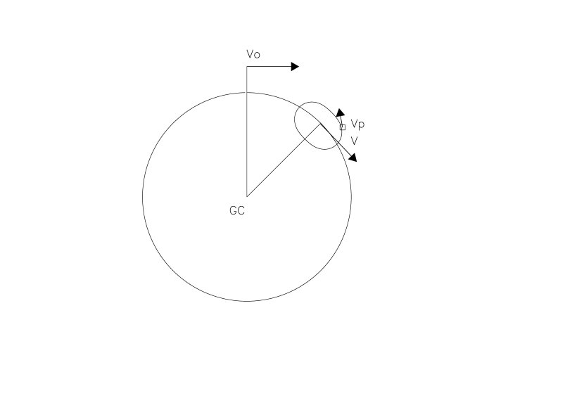
Figure 1: Epicycle orbit around an equilibrium point rotating with circular velocity V around the Galactic Center. V_p represents the perturbed velocity.

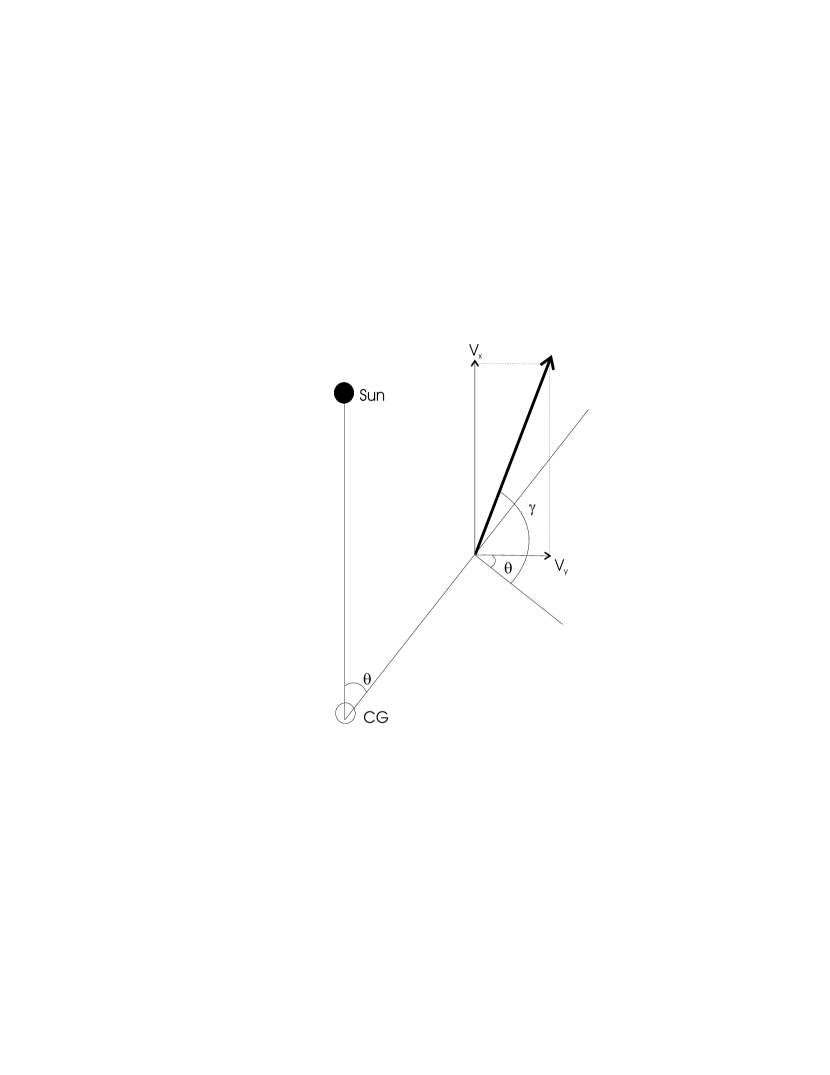
Figure 2: The geometry of the velocity vectors. We adopt a usual convention with the Y axis oriented along the circular rotation at the solar position, and the X axis in the galactic radial direction, oriented towards external regions. One can see that $\gamma=\theta+tan^{-1}(V_{x}/V_{y})$, with $\theta=sin^{-1}(y/R)$

In the hypothetic case $a=b$, $\gamma$ would increase linearly with time, with a slope $\kappa$. In the case $a/b$ = 1.5, $\gamma$ is a smooth increasing function of time, with a slope that on the average is equal to $\kappa$, since in a time $T=2\pi/\kappa$, $\gamma$ varies $360^{o}$. If all the clusters had a same starting angle, in a plot of $\gamma$ versus age of the clusters the slope of the fitted line would give directly the value of $\kappa$.

The present day velocity vector of an open cluster with respect to the Sun, projected on the galactic plane, is obtained from the data given in the catalog: it is the sum of the radial velocity projected on the plane, and of the velocity in the plane of the sky, derived from proper motion and distance, also projected on the galactic plane. We first convert the velocities to the Local Standard of Rest (LSR). Different sets of solar velocity components ($u,v,w$) with respect to the LSR are recommended in the literature, like the Standard Solar Motion, with ($u,v,w$) = (-10.4, 14.8, 7.3) (in kms^-1, Mihalas & Binney, 1981), (-10.4, 5.3, 7.3) from the analysis of the Hipparcos data by Dehnen et al. (1987), (-9.7, 5.2, 6.7) also based on Hipparcos data by Bienaymé (1999), or (-9.9, 12.1, 7.5) according to Abad et al.(2003), among others. Since differences of a few kms^-1 between the diverse systems only occur in the $v$ component, we varied it to verify how it affects our results. We finally adopted $v$ = 9.0 kms^-1, since this value corresponds to a minimum of the rms deviation of the adjusted points in the determination of the epicycle frequency. However, this choice is not critical for our results; almost the same values of epicycle frequencies were obtained with $v$ in the range 6 to 12 kms^-1. Interestingly, we have another argument based on the new ideas of the present paper in favor of this intermediate value of $v$ between the extreme ones, 5 and 15 kms^-1. The perturbation velocities are rotating, and since the clusters span a range of ages, even if their initial velocities had some preferential direction, the present direction must be almost random (or cover almost uniformly the range -180^∘ to 180^∘). However, if we adopt an artificially incorrect value for $v$, like 0 kms^-1 or 20 kms^-1, the present day distribution becomes either very concentrated around $\pm$ 180^∘ or around 0^∘. This experiment tells us that the correct $v$ must be near the center of the range 0 kms^-1- 20 kms^-1.

A further step in the treatment of the velocity vectors is their transformation to the local reference frame of each cluster, as illustrated in Figure 2. The new frame has an axis in the local direction of rotation and the other in the local radial direction. This step includes the corrections for differential rotation, described below. The local frame of the clusters at present time is the most convenient one to start numerical integration of orbits. However, for the other use of the velocity vectors, which is the direct determination of the epicycle frequency, a small correction is still required to place the velocity in the frame of reference of the guiding center, as later discussed.

In this work, we do not take into account the velocities perpendicular to the plane; only the velocity components projected on the galactic plane are investigated.

3.1 Corrections for differential rotation and local frame of reference

After electing a rotation curve, we subtract from the observed velocity of a cluster the velocity expected from pure circular rotation at its position; what is left is the perturbation velocity. This is not different from what DL called correction for differential rotation. The corrections can be made in different ways; the one that we adopted is to compute, for the longitude and distance of each cluster, the expected U and V velocity components, assuming that the cluster presents pure circular rotation, and subtracting the velocity components (0, V₀) of the LSR. Of course, the perturbation velocity vectors that we derive (observed - expected velocities) depend slightly on the choice of the galactic parameters $R_{0}$, $V_{0}$, $(dV/dR)_{0}$ (the radius of the solar orbit, the rotation velocity of the LSR around the galactic center, and the slope of the rotation curve, respectively). However, we are dealing with second order (or differential) effects; if we adopt a rotation curve that is too low or too high, the LSR velocity and the expected cluster velocity are affected in a similar way, and the computed perturbation velocity does not change too much. As already discussed, once a perturbation velocity vector is established, its angle $\gamma$ will be measured with respect to the local rotation direction.

Since the epicycle frequency depends strongly on the galactic radius (equation 1), we must select the clusters in a narrow range of radius, to be able to observe a well defined rotation of the perturbation velocity. We must make a compromise, since too narrow galactic radius ranges will contain only a few clusters. After a number of experiments, we found that a radial extent of the order of 0.6 - 1 kpc is convenient. A special radius range is the one that contains the Sun (let us say, the range $R_{0}\pm$ 0.4 kpc), because it is not affected by differential rotation; whatever the rotation curve we choose, the expected circular rotation velocity of the clusters is the same of LSR rotation around the galactic center.

3.1.1 Rotation curves

For radius ranges (or rings) relatively distant from $R_{0}$, the choice of the rotation curve is relevant. Our task is risky, since we are willing to observe perturbations of the order of 10 kms^-1 over a line-of-sight projection of rotation velocity of the order of 130 kms^-1. For instance, if the true rotation velocity of the Galaxy in a ring is larger than the one that we use for the corrections, the perturbation velocities are under-corrected in the direction of $\eta^{\prime}$ and the observed $\gamma$s will tend to be closer to zero than they should be. The effect is similar to the one that we described previously, concerning the $v$ component of the solar velocity. In principle, the fact that under-corrections or over-corrections tend to destroy the ”normal” distribution of present day angles of the velocity vectors could be used as a guide to select the correct rotation curve. But this is not the purpose of the present work.

Anyway, in order to check the effect of the differential rotation corrections on the derived epicycle frequency, we performed the calculations over a grid of rotation curves. We varied $R_{0}$ from 7.0 to 8.5 kpc, in steps of 0.5 kpc, and $V_{0}$ from 170 to 250 kms^-1, in steps of 10 kms^-1. The method is very similar to that of DL for the determination of the pattern rotation speed; for each point of the grid we make use of a rotation curve that passes at the corresponding ($R_{0}$, $V_{0}$) and fits the observed CO data taken from Clemens (1985); the same set of rotation curves of DL was used here. These are curves directly derived from observations, with the rotation velocities recomputed for each adopted ($R_{0}$, $V_{0}$). A simple and smooth analytical expression was fitted to each of these curves, in order to be able to compute the corresponding ”theoretical” epicycle frequency. We refer to these curves as CO-based curves or smooth curves. We also performed a number of experiments with constant velocity curves, or pure ”flat”curves.

Not all the points of this grid of rotation curves and radial ranges produce a valid measurement of the epicycle frequency. We later discuss in more detail an example with a specific choice of $R_{0}$, in order to clarify what we consider a valid measurement.

3.1.2 The reference frame of the guiding center

The equations 2 to 5 are valid in the reference frame of the guiding center of the epicycle motion, which does not coincide with the local reference frame at present epoch. A small correction to the angle $\gamma$, corresponding to a change of the velocity component in the $\eta$ direction, is required for this last frame conversion. The velocity shift only affects the direction of circular rotation, since the local frame and the the frame of the guiding center have the same (zero) radial velocity.

The expression for the correction is derived in Appendix A, based on the equations of motion derived by Makarov et al.(2004, hereafter MOT). It should be noted that the MOT’s equations are mainly intended to describe the positions of stars as a function of time. In the analysis of positions, a secular drift appears and is quite important, this being the reason for the stretching of open clusters. In the present work, we are not dealing with positions, but only with velocities (our analysis is based on plots of velocity directions as a function of age). Velocities are not affected by secular terms like positions are; this is why young associations that are considerably stretched (like Sco-Cen, and the stellar streams) are easily recognized through their common spatial velocities. In our particular case the present day position of the particles (clusters) coincide with the origin of the individual local frame. As we move towards the past or the future, the local frame rotates with a constant circular velocity and the particles move out from the origin.

It is shown in Appendix A that the amplitude of the correction $\delta\gamma$ to the present day angles, that we apply to each point on the graphs like figure 4, has an rms value about 15^∘, and is on the average equal to zero. Since the tolerance adopted in our analysis (section 3.3) for a point to be considered as belonging to a fitted line is 20^∘, and the fitted parameters ($\kappa$ and $\varphi$) depend on many points, the errors that would be introduced by not performing the $\delta\gamma$ correction would be small. For such a small correction, a first order estimation of it is largely sufficient. For this reason, the fact that the correction is based on a theory that makes use of the Oort’s constants, of which we do not know a priory the exact values, is not relevant. The use of different sets of Oort’s constants produces minor differences in the corrections (as illustrated in Appendix A), that do not affect the fitted parameters.

3.1.3 The modulus of the velocity perturbation

The histogram of the modulus of the velocity vectors, or residual velocities after correction for differential rotation, is presented in Figure 3. The peak of the distribution is at about 10 kms^-1. In parts of the following study we remove from the sample the clusters with modulus larger than 20 kms^-1. The reason is that if the amplitude of the perturbation is large, the simple epicycle approximation is not valid. However, when we are dealing with numerical integration of the orbits, which do not rely on the epicycle approximation, this restriction is not needed. We also remove from the sample the too small velocities ($\mid V\mid<$ 3 kms^-1 ), since the velocity components would be of the same order of the measurement errors, and the error on the angle $\gamma$ could be large.

Figure 3: Histogram of the modulus of the residual velocity vectors of the open clusters in the galactic plane, after subtracting the normal rotation velocity at that radius.

3.2 The case $R_{0}$=7.5 kpc, and clusters near galactic radius R₀

The measurement of the epicycle frequency gives us a link between $R_{0}$ and $V_{0}$, like the well known link between the same parameters given by the Oort’s constants A and B. If we fix one of these parameters, we can derive the other. Recent work often adopts R₀ = 7.5 kpc (Racine & Harris, 1989, Reid, 1993, and many others). This shorter galactic scale, compared to the IAU recommended 8.5 kpc scale, is supported by VLBI observations of H₂O masers associated with the Galactic center. The distance to the Galactic center derived from infrared photometry of bulge red clump stars (Nishiyama et al. 2006) is R₀=7.52 $\pm$0.10 kpc, while astrometric and spectroscopic observations of the star S2 orbiting the massive black hole in the Galactic center taken at the ESO VLT (Eisenhauer et al., 2005) gives 7.94 $\pm$ 0.42 kpc.

Figure 4 (a,b,c) are plots of the angle of the perturbed velocity vector with the direction of circular rotation, as a function of age. In these examples, the galactic positions of the clusters were computed considering that R₀ = 7.5 kpc, and the plots a, b, c, show clusters selected in different ranges of galactic radius. In particular, the range shown in Figure 4b is 7.1 $<R<$ 7.9 kpc. As we already mentioned, this is a special radius range, since the choice of the rotation curve has no influence on the fitted $\kappa$. The positions and velocities in the galactic plane of the same sample of clusters are shown in Figure 5. In Figure 4a and 4c, the two lines represent the function (6), for a same value of $\kappa$, but different values of $\varphi$. When a line reaches the maximum angle that can be measured ($180^{o}$), it starts again at $-180^{o}$. In Figure 4b only one line was plotted, as it seems to be a dominant one, fitting alone 12 clusters, considering that a cluster is fitted if it is situated within $\pm 20^{o}$, in the vertical direction, from the line. The points situated around this line are reproduced in Figure 6 without the folding at multiples of 180^∘; 2 points slightly off the $\pm 20^{o}$ limit were included. The rms deviation of the points from the line is 14^∘. It can be noted from Figure 4 that for ages larger than 50 Myr, no points considered as not belonging to the line are closer than about 130^∘(or 9$\sigma$) from it. This justifies our method of ”isolating” a line to fit the theoretical function. In the present case the fitted value of $\kappa$ is 42.0 $\pm$ 4 kms^-1kpc^-1; this is the epicycle frequency at the solar radius, one of the main results reported here. The initial angle is 61^∘, in the frame of the guiding center, or a little more, about 80^∘ in the local frame of the clusters. This initial angle is in good agreement with what is obtained from a totally different method (Figure 4e). The probability of the apparent alignment of points being a chance coincidence is discussed in the next section.

Figure 4: Left-side (a,b,c): angle $\gamma$ between the perturbed velocity and the direction of circular rotation as a function of the age of the clusters. The lines represent the function (6) for different values of $\varphi$. The clusters were selected in different ranges of galactic radius, indicated in each frame. The fitted values of $\kappa$ were 46, 42 and 45 kms^-1kpc^-1 respectively. The right side frames are the histograms of initial velocities for the corresponding radius ranges, obtained by numerical integration of the orbits (section 3.4)

Figure 5: Observed position and perturbation velocity vectors of the clusters in the range of galactic radius 7.1$<R<$ 7.9 kpc. The radius range is indicated by full lines and the solar radius by a dotted line. In the text we refer to this region as the R = 7.5 kpc ring. The galactic center is not contained in the figure.

Figure 6: Angle $\gamma$ between the perturbed velocity and the direction of circular rotation as a function of the age of the clusters, for the clusters situated around the line shown in Figure 4b, with the 180^∘ folding removed. The adjusted line gives $\kappa$ = 42.0 $\pm$ 4 kms^-1kpc^-1 and $\varphi$ = 70^∘, which corresponds to an initial angle 61^∘ (Equation 6).

The fact that a reasonable number of points fall on a same line (for instance, 12 clusters within $\pm$ 20^o of the line that begins at 61^o) reveals that some process confines the direction of the initial velocity of the clusters to a same angle with respect to the direction of circular rotation, for periods of time of more than 100 Myr. We postpone for the moment the discussion on the nature of such process.

3.3 Probabilities of alignment in a random process

In the case illustrated in Figures 4b, the sample contains 52 clusters. The probability of 12 clusters being fitted by a theoretical line, as it happens in this case, is small. The probability of a point falling on a given line which has a ”thickness” of 40^o is 40/360 = 1/9. The probability of 12 points being on a given line, out of 52 experiments, or 12 successes and 40 failures, is [52!/(12! 40!)](1/9)¹²(8/9)⁴⁰, $\approx$ 7$\times 10^{-3}$.

In the example of Figure 4a, with a sample of 40 points, 2 lines have been fitted, with a total of 16 points on them. In a random process, the probability of falling on one of the two lines is 2/9. If 40 points are randomly placed on the diagram, the probability of 16 points falling on any one of 2 given lines (15 successes and 21 failures) is [40!/ (16! 24!)](2/9)¹⁶(7/9)²⁴ $\approx 5\times 10^{-3}$.

In the first example, one could argue that the problem cannot be reduced to that of throwing 52 points on graph and computing the probability of 12 of them being within a given distance of a line, since the line was not previously present; we fitted their parameters so that they pass through a group of points that resulted to be aligned. This is equivalent to reduce the number of ”successes”, for instance, we can choose 2 points to define the phase and slope of the line. In this case we require only 12 successes and 40 failures; the probability is still only about 3$\%$. In reality, the probability of the observed alignments of points being spurious can be discarded, since the fitted value of $\kappa$ are always very close to the ones expected from theory, and the initial phases are confirmed by another method. Furthermore, there is a continuous variation of $\kappa$ from one ring to the other; for instance, the clusters in figures 4a and 4b are not the same, since the galactic rings do not overlap, but the fitted slope changes smoothly from one ring to the other. We note that the choice of the number of fitted lines is arbitrary; similar conclusions can be obtained with 1, 2, or 3 lines. We also verified that our conclusions do not depend strongly on the ”thickness” of the lines; if we decide that points at distances up to 15^o or 25^o from a line are fitted points, the number of fitted points varies, but the change in the probability of being on a line by chance tends to compensate the variation, in the calculation of probability.

The simple analysis of probabilities tells us that we are not dealing with random alignments, but also warns us that we should not attempt to draw conclusions from cases with a small number of aligned points, like for instance less than half of the total number of points being on 3 candidate lines, or less than one third of the points being on two lines, within a tolerance of 20^o. When the number of clusters decrease, or when the galactic parameters or rotation curves are different from the correct ones, we are sometimes confronted with situations in which very different values of $\kappa$ seem to fit the points with about the same quality of the fit. This limits the number of galactic rings and the range of parameters that can be explored.

3.4 Numerical integration of the orbits and histograms of initial directions

The approximation described in the previous sections is useful to provide an estimate of the epicycle frequency without depending on a precise knowledge of the rotation curve. A rough idea of the distribution of initial velocity directions is obtained simply by looking at the starting angles of the fitted lines (at age=0).

To obtain the distribution of initial angles, a second method is to perform a numerical integration of the stellar orbits. For this integration, a first step is to obtain the axis-symmetric potential of the Galaxy, by integrating the force $V(R)^{2}/R$ based on the adopted rotation curve. In this way, the potential does not depend on any assumption on the different components of the Galaxy (disk, bulge, etc.). The present day position and velocity of a cluster define a quadrivector q(t) containing the polar coordinates, the radial velocity and the angular momentum, which are the initial conditions of the integration. In the integration, at each time step, $q(t+dt)$ is deduced from $q(t)$ using a Runge-Kutta IV method. The value of $dt$ is chosen so as to have about 360 points along a circle around the Galactic center. The integration is performed backward in time, for a total time equal to the age.

If the adopted rotation curve is close to the true one, the two methods should produce similar initial velocity distributions. Therefore, the comparison between the results of the two methods is a tool to make a choice among different rotation curves. As examples of histogram of initial velocity directions, those obtained with the same samples used in Figure 4 (a,b,c), are shown in Figure 4 (d,e,f, respectively). Note that we expect to obtain similar, but not precisely the same distribution of initial velocities with the two methods, since the methods rely on different simplifying assumptions. For instance, the numerical integration takes into account the present day galactic radius of individual clusters, while the slope-fitting method considers intervals of galactic radius, and supposes that the equilibrium radius of the circular orbit is approximately the center of the radius range. It should be remembered that the initial angle in the slope-fitting method is in the frame of reference of the guiding centers (Section 3.1.2).

The agreement between the two methods is found to be quite satisfactory when rotation curves with high values of $V_{0}$ (220, 230 kms^-1kpc^-1) are used, but become poor with small $V_{0}$, like 180 kms^-1kpc^-1.

3.5 Possible sources of errors

A source of uncertainty in the value of $\kappa$ that we obtain, in the examples that we discussed, illustrated in Figure 4, is that $\kappa$ depends on the definition of the LSR. It may happen that we are not using the best set of solar velocity components for the LSR corrections, in the choice described in section 3. The ”correct” LSR would be the reference frame that rotates around the Galactic center with the velocity of the rotation curve at R₀. It can be seen from Figure 2 that if we add a correction to $V_{y}$ (in the direction of rotation), the computed value of $\gamma$ will change. A small change in the LSR definition produces a same $\delta V_{y}$ for all the clusters, but different angles $\gamma$ are affected in a different way, so that the slope of the fitted lines in Figure 4 may change. The arguments which led us to adopt $v$ = 9 kms^-1 are explained in section 3.0. We verified that typically, if we add 1 kms^-1 to the $V_{y}$ component of each cluster, to mimic the effect of an error on the $v$ component of the solar motion, the fitted $\gamma$ is changed about 1 kms^-1kpc^-1. The error on $\kappa$ introduced by the uncertainty in $v$ is about $\pm$3 kms^-1kpc^-1.

It was mentioned in Section 3 that the ratio a/b is approximately 1.5, but the precise value depends on the adopted $\Omega$ and $\kappa$. A number of tests showed that a small variation of this ratio (like for instance taking a/b = 1.4) does not produce any change in the fitted values of $\kappa$, so that it was not even necessary to use an iterative procedure to determine $\kappa$. Similarly, in section 3.1.2 we commented that the correction $\delta\gamma$ for the frame of reference of the guiding centers depend on the Oort’s constants, which in turn depends on the adopted rotation curve. In this case too, these are second order effects, and an iterative procedure is not required. In principle, when a line is fitted to the observed points like in Figure 6, the scattering of the points due to the errors in radial velocities and proper motions contained in the catalog, as well as the small effects that we just mentioned, are taken into account in the error on the slope given by the least-square fitting. We consider that our final errors on $\kappa$ are $\pm$4 kms^-1kpc^-1.

Other effects like the possible perturbation of the orbits by the spiral structure (see eg Lépine et al, 2003), or the effects of the local wiggles of the rotation curve (section 3.8) are not considered here as errors of measurements, but the cause of discrepancies between the measured $\kappa$ and theoretical values expected from too smooth rotation curves.

3.6 Detailed analysis and the derived value of $V_{0}$

We expect that if a rotation curve is a good approximation of the true one, it will produce a match between the theoretical and observed $\kappa$, not only near $R_{0}$, but at other galactic radii as well. In Figure 7 we present $\kappa$ as a function of radius, obtained from the same slope-fitting method illustrated in Figures 4(a,b,c). We remark that all the determinations of $\kappa$ rely on this method, the numerical integration is used only in the statistics of initial velocities. The method does not give reliable results between 8.0 and 8.9 kpc, because the number of clusters becomes too small, and in addition, the number of initial phases seem to be larger. Only at 8.9 kpc we found again a reliable result. Although the observed epicycle frequencies do not depart much from those predicted (based on Eq. 1) by a smooth rotation curve with $V_{0}$= 220 kms^-1, the slope of $\kappa$ as a function of radius is steeper than that of smooth rotation curves. The data in Figure 7 was also fitted by a smooth $V_{0}$ = 230 kms^-1 rotation curve modified by the addition of a Gaussian minimum centered at 7.8 kpc and peak value 6 kms^-1 , the corresponding value of $V_{0}$ being about 225 kms^-1. The existence of a minimum is further discussed in a next section. We do not intend to present a precise fitting of it, but only to illustrate that it could be an explanation for the anomalous slope of $\kappa$. Such a minimum is almost not perceptible in the rotation curve (Figure 10).

Figure 7: Epicycle frequency measured at different galactic radii. The dashed lines represent the theoretical $\kappa$ corresponding to smooth rotation curves with $V_{0}$ = 230 kms^-1(upper curve) and 220 kms^-1 (lower curve) both with $R_{0}$ = 7.5 kpc. The dotted line correspond to the theoretical $\kappa$ obtained with a smooth rotation curve with $V_{0}$ = 232 kms^-1, to which a Gaussian minimum centered at 7.8 kpc has been added.

Interesting results are obtained by varying the rotation curves with a fixed $R_{0}$. Figure 8 presents the theoretical and observed epicycle frequency as a function of the adopted $V_{0}$, for a fixed $R_{0}$= 7.5 kpc. What we call here the theoretical $\kappa$ is the value obtained from direct use of equation (1), with $\Omega(R)$ given by the adopted rotation curve; the observed $\kappa$ is obtained from the slopes of lines in plots similar to those shown in Figure 4. For each $V_{0}$, the same rotation curve is used to determine the theoretical frequency and for the differential rotation corrections. Figure 8 turns clear how the best value of $V_{0}$ can be derived, and how the uncertainty on $\kappa$ affects this $V_{0}$ value.

Let us first analyse the case of pure flat rotation curves (V($R$)=V($R_{0}$)= constant). For such curves, it can be derived from equation (1) that $\kappa$ = $\sqrt{2}\Omega$. At $R_{0}$, $\Omega$ = $V_{0}/R_{0}$; the dashed line in Figure 8 gives $\kappa$ as a function of $V_{0}$, for flat curves with R₀ = 7.5 kpc. This line cuts the line of observed $\kappa$ at 42 kms^-1kpc^-1 and V₀ = 226 kms^-1. In other words, if the rotation curve were a flat one, our measurement of $\kappa$ = 42 $\pm$ 4 kms^-1kpc^-1 would imply that V₀ is 226 $\pm$ 15 kms^-1.

Figure 8: The epicycle frequency as a function of $V_{0}$ for different rotation curves, all based on $R_{0}$ = 7.5 kpc. The full line with positive slope is the theoretical prediction for the series of CO-based rotation curves with different values of $V_{0}$ (see section 3.1.1). The dashed line is the theoretical $\kappa$ for pure flat curves with different $V_{0}$. The full line with negative slope shows the observed values of $\kappa$, based on angle versus age fitting, like in Figures 4(a,b,c). The theoretical and observed $\kappa$ intersect at at about 226 kms^-1.

Besides the pure flat (slope zero) curves, another family of curves that we consider is that of smooth curves, obtained by fitting the CO data with different values of $V_{0}$ (section 3.1.1). The line representing the theoretical $\kappa$ for this family of curves also cuts the observed line at 226 kms^-1. The coincidence of the two ”theoretical” lines intersecting at 226 kms^-1 is not surprising, since the smooth curves for $V_{0}$ about 220-230 kms^-1 are very close to flat ones (see Figure 10).

3.7 Rotation curves with $R_{0}$ = 7.5 kpc at different galactic radii

We present in Figure 9 the observed values of $\kappa$ (based on figures similar to Figure 4) and theoretical values of $\kappa$ (derived from the family of CO-based curves) for two distinct ranges of radius, one smaller than $R_{0}$, 5.9 $<R<6.5$ kpc (dashed lines), and the other larger than $R_{0}$, 8.2 $<R<9.8$ kpc (dotted-dashed lines). The lines with positive slope are the theoretical ones. The two lines corresponding to $R$ = 6.2 kpc intersect at about $V_{0}$ = 220 kms^-1; while the two lines corresponding to $R$ = 9.0 kpc intersect at about 235 kms^-1; both values have errors $\pm$ 10 kms^-1 and are in agreement with $V_{0}$ = 226 kms^-1, previously obtained from the clusters situated near $R$ = 7.5 kpc, in Figure 6.

Figure 9: Theoretical and observed values of $\kappa$ as a function of $V_{0}$ of the CO-based rotation curves (all with $R_{0}$ = 7.5 kpc), for two distinct galactic radii: 6.2 kpc (dashed lines) and 9.0 kpc (dashed-dotted lines). The positive slope lines are the theoretical ones, and the negative slope are the observed ones, like in Figure 8.

3.8 Rotation curves with $R_{0}$= 7.0 , 8.0 and 8.5 kpc

An analysis similar to that of the previous subsections has been performed, adopting $R_{0}$ = 7.0 kpc, $R_{0}$= 8.0 kpc and $R_{0}$= 8.5 kpc. For each adopted $R_{0}$, families of smooth rotation curves with different values of $V_{0}$ (as explained in section 3.1.1) were used to derive the theoretical $\kappa$ at the radius $R_{0}$. On the other hand, the angle of the observed velocity perturbation with respect to the direction of circular rotation have been plotted, using the samples of clusters in the radius range $R_{0}~{}\pm$ 0.4 kpc. The study was also made for rings that do not coincide with $R_{0}$; the width of the rings was always about $\pm$ 0.4 kpc. In all the cases the figures look similar to Figure 9, with a rising theoretical line and a decreasing line of ”observed” $\kappa$. The intersection of the two lines is considered as the best estimate of $V_{0}$ for the given $R_{0}$. The results are summarized in Table 1.

Table 1: Values of $V_{0}$ for which the observed and theoretical $\kappa$ are equal, for different adopted $R_{0}$ and different radii of the galactic ring.

$R_{0}$	ring radius	best $V_{0}$	$\kappa$
kpc	kpc	kms-1	kms-1kpc${-1}$
7.0	5.7	195	50
7.0	7.0	230	47
7.5	6.2	220	48
7.5	7.5	225	42
7.5	9.0	230	35
8.0	6.7	225	48
8.0	8.0	230	40
8.5	7.3	210	42
8.5	8.5	245	42

It can be seen that the observed $\kappa$ at $R$(ring)= $R_{0}$ is almost the same for the different adopted $R_{0}$ (the average of the $R$= $R_{0}$ rings in Table 1 is $\kappa$=43 ). This is an expected result since the samples of clusters are the same in these cases, as the positions of the clusters are given relative to the Sun. And, as we already mentioned, when we study a ring at $R_{0}$, the rotation curve has only a second order effect in the determination of $\kappa$. The fact that a same best estimate of $V_{0}$ is obtained for $R_{0}$= 7.0, 7.5 and 8.0 kpc is an indication that this value is a robust result. Furthermore, the fact that for $R_{0}$ = 7.5 and 8.0 kpc almost the same value of $V_{0}$ is obtained from two different rings is an indication that the smooth rotation curves that we are using in these cases are close to the real ones.

3.9 A wiggled rotation curve and the Oort’s constants

It is well accepted that the rotation curve presents irregularities in the solar neighborhood. According to Olling and Merrifield (1998), there is a minimum at about $R_{0}$ + 3 kpc, and a step to higher rotation velocities at about $R_{0}$ + 4 kpc. Honma and Sofue 1997) used the same method of Merrifield (1992), and both groups obtain a step-like increase of rotation velocity, but at different radius: about 1.2 $R_{0}$ (HS) or about 1.5 $R_{0}$ (M). Brand & Blitz (1993) found the deepest minimum at about 1.15 $R_{0}$, and the start of a step-like increase at about 1.3 $R_{0}$. Amaral et al. (1996), based on an analysis of OH/IR stars, found the minimum at 1.07 $R_{0}$. We propose the curve presented in Figure 10, which contains a minor wiggle represented by a Gaussian minimum centered at 7.8 kpc with a half-width of 1kpc, and depth 8 kms_-1. Such a wiggle produces a reasonable fit of the epicycle frequency (see Figure 7), and the general curve fits the Clemens (1985) data, excepting for the minimum at about 8.5 kpc. It should be noted that Clemens did not use the same VLSR transformation that we adopted in the present work, and that the we applied corrections for the different $R_{0}$ that are only strictly valid for the data inside the solar circle.

In most of the descriptions that we mentioned, the minimum is at 1.1 $R_{0}$ or beyond. So up to $R_{0}$ the curve is still quite flat, and we believe that our analysis of the sample of clusters near $R_{0}$ is not seriously affected by the wiggles. Indeed, when we plot the angle $\gamma$ as a function of age, like in Figure 4, but using our curve with aminor wiggle to perform the differential rotation correction, the result looks very similar to Figure 4, except that the best fit of the slope of the lines gives us 41 kms^-1kpc^-1, instead of 42 kms^-1kpc^-1. This difference is well within the error bars.

Figure 10: The rotation curve of the Galaxy for $R_{0}$ = 7.5 kpc. The line is a fit to the CO data, using the empirical expression V= 240 exp(-(3.6/r)²) + 350 exp(-r/3.5 -0.12/r); the units are km^-1 and kpc. A very small wiggle was added, represented by a Gaussian minimum -8 exp(-[(r-7.8)/1.0]²), in order to better fit the epicycle frequecy data (Figure 7). Including this term, $V_{0}$ = 226 kms^-1 precisely at $R_{0}$, but outside the minimum $V$ =230 kms^-1.

An important aspect of the minimum in the curve is that it could explain the apparent contradiction between our results and previous results based on the Oort’s constants. The value of $V_{0}$ that we obtain may seem too high, since it corresponds to $V_{0}/R_{0}$ = 30.1 (the units are kms^-1kpc^-1 in what follows). In a first order approximation, the parameters V₀ and R₀ are linked together through the Oort’s constants A and B, which are determined by observations (V₀/R₀ = A - B, (dV/dR)_R0 = -A-B ). A value of A-B which seemed to be well established is 26, confirmed by recent observations of a different nature (Kalirai et al., 2004) which give 25.3. Feast & Whitelock (1997) obtained 27.2 based on Hipparcos proper motions of Cepheids. However, Olling and Merrifield (1998) verified that the Oort’s constants A and B differ significantly from the general $V_{0}/R_{0}$ dependence, in the solar neighborhood. They attributed this effect to an anomaly in the local gas distribution. Olling & Dehnen (2004) showed that the most reliable tracers of the ”true” Oort’s constants are the red giants, and derived A-B = 33. Another previous determination with high value of A-B is that of Backer & Sramek (1999), who measured the proper motion of Sgr A, at the Galactic center, equal to 6.18 $\pm$ 0.19 mas yr^-1, equivalent to 29.2 $\pm$ 0.9. This is an interesting result since it does not depend on local wiggles. Branham (2002) obtains $\Omega$= 30.3, Fernández et al. (2001),$\Omega$ =30, and Miyamoto and Zu (1998), $\Omega$ = 31.5, all of them from the kinematics of OB stars. Meztger et al. (1998) obtained 31 from Cepheid kinematics, and Mendez et al. (1999) obtained 31.7 from the Southern Proper Motion Program. We conclude from this discussion that the value of $V_{0}$ that we obtain, and our choice $R_{0}$ = 7.5 kpc, are not in contradiction with the constraints of the Oort’s constants.

As we already mentioned, one of the main properties of the wiggles is a minimum at about 1.1-1.2 $R_{0}$, observed by different authors and using different tracers. We only insist here on the existence of the minimum because it has not always been recognized, possibly because there seems to be no obvious reason for it. The existence of this sharp (half-width about 1.0 kpc) minimum could possibly be related to corotation. This resonance is a frontier between two regions of the galactic disk, one in which the matter flows towards the center, and one in which the matter flows towards external regions. This tends to form a ”vacuum” around corotation, as confirmed by hydrodynamic simulations (eg. Lépine et al. 2001). If less gas is present, less stars form, and after a few billion year a ”gap” ring with a smaller stellar density forms.

3.10 Statistics of initial directions

Typically, a ring with a width about 0.8 kpc contains 3 or 4 main directions of initial velocity perturbation, seen as peaks in the histograms. A preliminary analysis of the position on the galactic plane where open clusters were born, indicates that at least two different directions can originate from a same position in the galactic plane, at a same epoch. It was shown by DL that the clusters were born in spiral arms. We can now say that a same spiral arm can produce star clusters going in different directions. However, this kind of analysis is difficult to perform, since the samples become very small when narrow bins of ages and initial positions are considered.

Different rings may have different main directions, but some general tendencies can be observed. Figures 11 to 13 present the distribution of initial velocities in the local (U,V) frame of each cluster, for different ranges of radius, obtained by numerical integration. One is the local region, from 7.1 to 7.9 kpc (Figure 11), which has already been studied in detail, and is supposed to include the corotation radius. Another region, from 5.0 to 7.1 kpc (Figure 12) is inside the corotation circle. We consider a large galactic radius interval to obtain better statistics. Finally, in Figure 13 we show the distribution for clusters in the radius range 8.1 to 12 kpc, external to the corotation circle. One can see some preferential or non-random directions, which are the basis of the present work, since they offer the possibility of measuring the epicycle frequencies. Although the statistics are poor, it does not seem that a description in terms of pure ellipsoids would be an adequate one.

Clear differences appear between the three regions, with dominant positive U velocities at large galactic radii, and dominant negative U velocities in the internal region. There seems to be a change of about 180^∘ in the main velocity direction in the comparison of internal and external regions (from -50^∘ to + 130^∘). This is in general agreement with the idea that outside corotation, the spiral arms tend to pull the galactic material towards the exterior, while inside corotation the arms pull the material towards the center.

In principle, we might expect that the clusters start their life traveling along the spiral arms, so that they would not leave the arms before the brightest stars reach the end of their life. This would contribute to the well defined visible aspect of the arms. DL showed that if we select clusters with ages smaller than 20 Myr, the spiral structure appears clearly, while for ages larger than 30 Myr, it almost disappears. This time scale is comparable to the time required for a velocity vector to change its direction by 90^∘, which is 1/4 of the epicycle period. Interestingly, the dominant initial directions for the internal regions of the Galaxy satisfy the condition above. If we consider the vector sum of the circular velocity and of the perturbation velocity, for instance a vector with modulus about 230 kms^-1 in the V direction plus a perturbation with modulus 15 kms^-1 in the direction -70^o or in the direction -140^o (main directions seen in Figure 12), the resulting velocity is approximately along the spiral arms, considering a typical pitch angle of about 14^o.

Figure 11: Distribution of initial velocities of clusters in the galactic radius range 7.1 to 7.9 kpc

Figure 12: Distribution of initial velocities of clusters in the galactic radius range 5.0 to 7.1 kpc

Figure 13: Distribution of initial velocities of clusters in the galactic radius range 8.1 to 12.0 kpc

4 Conclusions

The study of samples of open clusters situated in small intervals of galactic radius or rings with width $<$ 1 kpc, reveals the presence of several sequences of 4 to 12 clusters that have been formed with a same initial direction of the perturbation velocity, as measured with respect to the direction of circular rotation. The expected rotation of the perturbation velocity vector from the epicycle theory can be observed in plots of the angle versus age of the clusters. In such plots, the sequences of clusters along lines that correspond to a same initial angle span ranges of ages of about 40 to 150 Myr. In a given ring, usually 2, 3 or more such preferential directions are observed. Probably, the initial angles are dictated by the local hydrodynamics in the spiral arms. The observations suggest that portions of the shock waves associated with the arms are coherent, or keep the same characteristics, during period of times of more than 100 Myr. Therefore, the observations provide an argument in favor of star formation triggered directly by the spiral shocks, and not by secondary processes like the explosion of supernovae.

If we average the initial direction of the perturbation velocity over a relatively large range of galactic radius (a few kpc), the individual coherent groups become less prominent, or average out, but a broad general distribution of initial directions appears, with a peak at about -70^o, for galactic radii smaller than R₀ (or smaller than the corotation radius). This particular initial direction helps the arms to keep their sharply defined aspect, since the clusters do not move out from the arms before the bright short-lived stars reach the end of their life.

The property of the cluster formation mechanism of producing initial perturbation velocities in a given direction for groups of clusters spanning a range of ages allows us to perform a direct determination of the epicycle frequency $\kappa$ in the galactic disk. This measurement shows only a minor dependence on the rotation curve which is used to perform the corrections for differential rotation, to find the perturbation velocity. For a given rotation curve, there are two ways of obtaining the epicycle frequency at a radius $R$. One is to make direct use of the expression for $\kappa$ as a function of $\Omega$ and its derivative, and the other uses the plots of the angle versus age of the open clusters. We compared the results obtained using different rotation curves, based on different values of $R_{0}$ and of $V_{0}$. If we fix for instance $R_{0}$ and vary $V_{0}$, we can find a best value of $V_{0}$, for which the ”observed” and the ”theoretical” values of $\kappa$ coincide.

If $R_{0}$ = 7.5 kpc is adopted, using the sample of clusters in the range $7.1<R<7.9$ kpc, we find $V_{0}$= 226$\pm$15 kms^-1. The same value of $V_{0}$ is obtained when we adopt $R_{0}$ = 7.0 kpc or $R_{0}$ = 8.0 kpc. Therefore, $V_{0}$= 226$\pm$15 kms^-1 is a robust result, which does not depend on the precise choice of $R_{0}$, in the 7-8 kpc range.

We examined samples situated in rings with different galactic radii; for instance with mean radius between 6 and 8 kpc. The rotation curve $R_{0}$ = 7.5 kpc , $V_{0}$= 226 kms^-1, with a minimum at 7.8 kpc is found to be a satisfactory one, since it predicts values of $\kappa$ that are consistent with the observed ones, not only at $R_{0}$, but also at these different galactic radii. The ratio $V_{0}/R_{0}$ that we recommend is 30.1 kms^-1kpc^-1, which is larger than that ”classical” value obtained from the Oor’s constants (A-B), 25 kms^-1kpc^-1. However, as we discussed in a previous section, there are many recent measurements that result in $V_{0}/R_{0}$ close to 30 kms^-1kpc^-1, including a method that does not depend on local irregularities of the rotation curve. The method to determine $V_{0}$ that we proposed is a new one, which is something much needed in view of the conflicting results that have been published in the last decade, almost always based on analyses of Oort’s constants.

5 Appendix A

The present paper deals with open clusters that are spread over distances distances of several kpc, so that it is convenient to use an individual frame of reference for each cluster, to describe their motion. The local frame is chosen to rotate around the galactic center with the velocity of the rotation curve at the radius where the cluster is at present epoch. In such a reference frame, in which $\xi_{0}$ = 0 and $\eta_{0}$ =0, the MOT’s equations of motion (see section 3.1.2) reduce to:

$$\xi=\frac{\eta_{0}^{\prime}}{2B}+\frac{\eta_{0}^{\prime}}{2B}cos(\kappa t)+\frac{\xi_{0}^{\prime}}{\kappa}sin(\kappa t)$$

$$\eta=\frac{\xi_{0}^{\prime}}{2B}-\frac{\xi_{0}^{\prime}}{2B}cos(\kappa t)+\eta_{0}^{\prime}\frac{A}{B}t$$

$$+\eta_{0}^{\prime}\frac{A-B}{\kappa B}sin(\kappa t)$$

where A and B are the Oort’s constants. Taking the derivative:

$$\xi^{\prime}=\frac{\eta_{0}^{\prime}\kappa}{2B}sin(\kappa t)+\xi_{0}^{\prime}cos(\kappa t)$$

$$\eta^{\prime}=\frac{\xi_{0}^{\prime}\kappa}{2B}sin(\kappa t)+\eta_{0}^{\prime}\frac{A}{B}-\eta_{0}^{\prime}\frac{A-B}{B}cos(\kappa t)$$

The only non-harmonic term is $\eta_{0}^{\prime}\frac{A}{B}$, a term that does not increase with time and represents a shift in velocity, which corresponds to the change from the local frame to the frame of the guiding center (the frame in which the motion is described by pure harmonic functions in both axes). At the instant t=0 the velocity in the local frame is ($\xi_{0}^{\prime},\eta_{0}^{\prime}$) and in the frame of the guiding center ($\xi_{0}^{\prime},\eta_{0}^{\prime}[1-\frac{A}{B}]$).

The initial angle $\gamma$ in the frame of reference of the guiding center is:

$$\gamma_{0GC}=atan(\frac{\xi_{0}^{\prime}}{\eta_{0}^{\prime}[1-\frac{A}{B}]})$$

so that:

$$\delta\gamma=atan(C\times tan[\gamma_{0}])-\gamma_{0}$$

where $\delta\gamma$ is the correction to $\gamma_{0}$ needed to convert it from the local reference frame to that of the guiding center. The constant $C$ obtained using the classical values of the constants A =15 kms^-1kpc^-1 and B= -11 kms^-1kpc^-1 (Mihalas & Binney, 1981, chapter 8) is 0.42; using the Oort’s constants adopted by MOT, A= 12 kms^-1kpc^-1 and B= -15 kms^-1kpc^-1, $C$= 0.55. since only an order of magnitude is needed, we can adopt $C$= 0.5. The function $\delta\gamma$ is illustrated in Figure A1; its average is zero, its maximum about 24^o and rms value 15^o in the worst case ($C$= 0.42).

Figure 14: Correction to the angle $\gamma$ to move it to the reference frame of the guiding center of the epicycle motion, as a funtion of $\gamma$. The dashed line is with $C$=0.55, full line with $C$=0.42 (see Appendix).

References

- (1)
- (2) Amaral, L.H., Ortiz, R., Lépine, J.R.D., Maciel, M., 1996, MNRAS 281, 339
- (3)
- (4) Backer, D.C., Sramek, R.A., 1999, ApJ 524, 805
- (5)
- (6) Bienaymé, 1999, A&A 341, 86
- (7)
- (8) Binney, J., Tremaine, S., 1987, Galactic Dynamics, Princeton University Press, Princeton, New Jersey.
- (9)
- (10) Brand, J., Blitz, L., 1993, Atron. Astrophys. 275, 67
- (11)
- (12) Branham Jr., R.L., 2002, ApJ 570, 190
- (13)
- (14) Clemens D. P., 1985, ApJ 295, 422
- (15)
- (16) Dias, W. S., Assafin, M., Lépine, J.R.D., Alessi, B. S., 2002, A&A 388, 168
- (17)
- (18) Dias, W. S., Assafin, M., Florio, V., Alessi, B. S., Libero, V., 2006, A&A 446, 949
- (19)
- (20) Dias, W. S., Lépine, J.R.D., 2005, ApJ 629, 825
- (21)
- (22) Dias, W. S., Lépine, J.R.D., Alessi, B. S., 2001, A&A 376, 441
- (23)
- (24) Dias, W. S., Lépine, J.R.D., Alessi, B. S., 2002, A&A 388, 168
- (25)
- (26) Eisenhauer,F., Genzel, R., Alexander, T, + 18 authors, 2005, ApJ, 628, 246
- (27)
- (28) Feast, M., Whitelock, P., 1997, MNRAS 291, 683
- (29)
- (30) Fernández, D., Figueras, F., & Torra, J., 2001, A&A 372, 833.
- (31)
- (32) Honma, M.,& Sofue, Y., 1997, Publ. Astron. Soc. Japan 49, 453
- (33)
- (34) Kalirai, J.S., et al., 2004, ApJ 601, 277
- (35)
- (36) Lépine, J.R.D., Acharova, I.A. , Mishurov, Yu.N., 2003, ApJ 589, L210
- (37)
- (38) Lépine, J.R.D., Mishurov, Yu.N., & Dedikov, S.Yu., 2001, ApJ 546, 234.
- (39)
- (40) Lynga, G., 1987, Computer Based Catalogue of Open Cluster Data, 5th ed., (Strasbourg; CDS)
- (41)
- (42) Makarov, V.V., Olling, R.P., Teuben, P.J., 2004, MNRAS 352, 1199
- (43)
- (44) Méndez, R.A., Platais, I., Girard, T.M., Kozhurina-Platais, V., van Altena, W.F.,1999, ApJ 524, L39
- (45)
- (46) Mermilliod, J. C., 1995, in Information and On-Line Data in Astronomy, ed. D. Egret & M.A. Albrecht (Dordrecht: Kluwer), 127
- (47)
- (48) Merrifield, M.R., 1992, AJ 103 (5), 1552
- (49)
- (50) Metzger, M. R., Cadwell, J.A.R., Schechter, P.L., 1998, ApJ 115, 635
- (51)
- (52) Mihalas, D., Binney, J.J., 1981, Galactic Astronomy, 2nd ed. San Francisco: Freeman
- (53)
- (54) Miyamoto, M., Zhu, Z., 1998, ApJ 115, 1483
- (55)
- (56) Nishiyama, S., Nagata, T., Sato, S., et al., 2006, ApJ 647, 1093
- (57)
- (58) Olling, R.P., Merrifield, M.R., 1998, MNRAS 297, 943
- (59)
- (60) Olling, R.P., Dehnen, W., 2003, ApJ 599, 275
- (61)
- (62) Paunzen, E.; Netopil, M., 2006, MNRAS 371, 1641
- (63)
- (64) Racine, R.; Harris, W. E., 1993, AJ 98, 1609
- (65)
- (66) Reid, M.J., 1993, ARA&A, 31, 345
- (67)