Role of the $\rho$ meson in the description of
pion electroproduction experiments at JLab

Abstract

We study the $p(e,e^{\prime}\pi^{+})n$ reaction in the framework of an effective Lagrangian approach including nucleon, $\pi$ and $\rho$ meson degrees of freedom and show the importance of the $\rho$-meson $t$-pole contribution to $\sigma_{T}$, the transverse part of cross section. We test two different field representations of the $\rho$ meson, vector and tensor, and find that the tensor representation of the $\rho$ meson is more reliable in the description of the existing data. In particular, we show that the $\rho$-meson $t$-pole contribution, including the interference with an effective non-local contact term, sufficiently improves the description of the recent JLab data at invariant mass $W\lesssim$ 2.2 GeV and $Q^{2}\lesssim$ 2.5 GeV${}^{2}/c^{2}$. A “soft” variant of the strong $\pi NN$ and $\rho NN$ form factors is also found to be compatible with these data. On the basis of the successful description of both the $\sigma_{L}$ and $\sigma_{T}$ parts of the cross section we discuss the importance of taking into account the $\sigma_{T}$ data when extracting the charge pion form factor $F_{\pi}$ from $\sigma_{L}$.

I Introduction.

The motivation of many experiments Brauel:1979zk ; Bebek:1977pe ; Volmer:2000ek ; Huber:2003kg ; Horn:2006tm ; Tadevosyan:2007yd on forward pion electroproduction at large $Q^{2}$ is the study (through measurements close to the pion mass shell) of the pion charge form factor $F_{\pi}(Q^{2})$. For values of the $s$-channel $p+\gamma^{*}$ energy $W$ above the resonance region and for small momentum -k ($k^{2}=t$) transfered to the nucleon spectator the longitudinal part $\sigma_{L}$ of the cross section is dominated by the $t$-channel quasi-elastic mechanism (see Fig. 1). In this case the $\pi NN$ strong form factor $F_{\pi{\scriptscriptstyle NN}}^{2}(t)\approx 1$ is a slowly varying function at $|t|\approx M_{\pi}^{2}$ and

$$\sigma_{L}\sim\frac{|t|F_{\pi{\scriptscriptstyle NN}}^{2}(t)}{(t-M_{\pi}^{2})^{2}}\sigma_{e\pi}^{\rm free}\,,\quad\quad\sigma_{e\pi}^{\rm free}\sim F_{\pi}^{2}(Q^{2})\,,$$ (1)

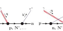
(a)                                         (b)                                           (c)

Figure 2: (color online). Feynman diagrams (“Born approximation”) for the pion electroproduction off the nucleon.

where $\sigma_{e\pi}^{\rm free}$ is the free $e\pi$ cross section. However, with currently available data Brauel:1979zk ; Bebek:1977pe ; Volmer:2000ek ; Huber:2003kg ; Horn:2006tm ; Tadevosyan:2007yd on the Rosenbluth separation of $\sigma=\sigma_{L}+\sigma_{T}$ the situation is not so simple. For comparison of data to theoretical predictions one should calculate both $\sigma_{L}$ and $\sigma_{T}$ parts of the cross section at least on the basis of a sum of the $s(u)$- and $t$-pole diagrams depicted in Fig. 2. It should be noted that the $s(u)$-channel contributions (Figs. 2(b) and 2(c)) to the forward pion cross section are suppressed Speth:1995er only at considerably high $Q^{2}$, i.e. in the region $Q^{2}\gtrsim$ 2 - 3 GeV²/c², where the product of corresponding vertex form factors and propagators drop faster in $Q^{2}$ ($\sim Q^{-n}$, $n\gtrsim$4) as compared to the $\sim Q^{-2}$ behavior of the pion form factor $F_{\pi}(Q^{2})$. In this $Q^{2}$ region the forward pion cross section is not as large as for smaller $Q^{2}\lesssim$ 1 GeV²/c² studied earlier Brauel:1979zk ; Volmer:2000ek , and until recently the available data on Rosenbluth separation were too poor Volmer:2000ek ; Huber:2003kg to be a reliable basis for the evaluation of $F_{\pi}(Q^{2})$.

The high quality data recently obtained at JLab Horn:2006tm ; Tadevosyan:2007yd for $Q^{2}=$ 1.6 and 2.45 GeV²/c² can considerably aid in the study of $F_{\pi}(Q^{2})$. However, at the values $W=$ 1.95 and 2.2 GeV characteristic of the high $Q^{2}$ JLab data (old and new) the kinematical limit for the momentum transfer $t_{c}\approx-(0.1-0.15)$ GeV²/c² is not so close to the pion pole position as is the case for low $Q^{2}\lesssim$ 1 GeV²/c². Thus the vertex dependence on $t$ for all the diagrams in Fig. 2 becomes very important for the extraction of the pion form factor $F_{\pi}(Q^{2})$ from the data on $\sigma_{L}$.

In this context the existing data on $\sigma_{L}$ and $\sigma_{T}$ available now Volmer:2000ek ; Horn:2006tm ; Tadevosyan:2007yd for a large region of momentum transfers $0.05\lesssim-t\lesssim 0.5$ GeV²/c² can also be used for the study of the strong meson-nucleon form factors $F_{\pi{\scriptscriptstyle NN}}(t)$, $G_{\rho{\scriptscriptstyle NN}}(t)$ and $F_{\rho{\scriptscriptstyle NN}}(t)$ in parallel to the study of $F_{\pi}(Q^{2})$. The direct measurement of these form factors would be very useful for both meson-exchange models of the nuclear force Machleidt:1987hj and of exchange currents in nuclei Riska:1989bh . Cutoff parameters $\Lambda_{{\scriptscriptstyle MNN}}$ ($M=\pi$ or $\rho$) used in the monopole parametrization

$$F_{\pi{\scriptscriptstyle NN}}(t)=\frac{F_{\pi{\scriptscriptstyle NN}}(0)}{1-t/\Lambda_{\pi{\scriptscriptstyle NN}}^{2}}\,,\quad F_{\rho{\scriptscriptstyle NN}}(t)=\frac{F_{\rho{\scriptscriptstyle NN}}(0)}{1-t/\Lambda_{\rho{\scriptscriptstyle NN}}^{2}}$$ (2)

are presently known only indirectly from data and values of $\Lambda_{{\scriptscriptstyle MNN}}$ are varying in a wide interval of $M_{\rho}\lesssim\Lambda_{{\scriptscriptstyle MNN}}\lesssim 2M_{\rho}$ (exchange currents in nuclei are usually fitted with soft form factors with $\Lambda_{{\scriptscriptstyle MNN}}\approx M_{\rho}$, while the nucleon-nucleon interaction models require harder form factors with $\Lambda_{{\scriptscriptstyle MNN}}\approx$ (1.5 - 2)$M_{\rho}$). On the other hand, in the constituent quark model (CQM) LeYaouanc:1972ae ; Ackleh:1996yt ; Neudatchin:2004pu the cutoff parameter $\Lambda_{{\scriptscriptstyle MNN}}$, at least for form factors at small values of $-t\lesssim$ 0.3 GeV²/c², is determined by the radius $b$ of the three-quark system and for realistic values $b\approx$ 0.5 - 0.6 fm one obtains $\Lambda_{{\scriptscriptstyle MNN}}^{2}\approx$ 0.5 - 0.7 GeV²/c².

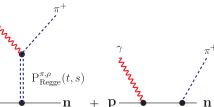
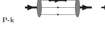
Figure 3: (color online). Factorization of the amplitude of pion electroproduction off the nucleon in the Regge model Vanderhaeghen:1997ts .

(a)                                         (b)                                     (c)

Figure 4: (color online). Microscopic interpretation of $t$- and $s$-channel processes within the quark model. Thick lines indicate the propagation of a large photon momentum $q$ through separate partons inside the nucleon.

In Refs. Neudatchin:2004pu ; Obukhovsky:2005sa it was shown that the recent JLab data on forward pion electroproduction Volmer:2000ek are compatible with a soft $\pi NN$ form factor. However, in Ref. Volmer:2000ek the data were described on the basis of a Regge model modified by introducing a common electromagnetic form factor $F_{\pi}(Q^{2})$ for both $t$-channel and “reggeized” $s$-channel amplitudes Vanderhaeghen:1997ts as is schematically shown in Fig. 4. In this model proposed by Vanderhaeghen, Guidal and Laget (VGL) there are no constraints on the maximum value of $|t|$ as the $t$-dependence of the cross section is determined by the $t$- (and $s$-) behavior of the $\pi$- and $\rho$-Regge trajectories. The model of VGL offers a satisfactory explanation of both photo- and electroproduction data for pions in a large interval of $t$ including the longitudinal part of the forward pion cross section $\sigma_{L}$ measured at JLab, but fails in explaining the transverse part $\sigma_{T}$. The prediction for $\sigma_{T}$ is about an order of magnitude smaller than measured values. At small $|t|\lesssim$ 0.3 GeV²/c² a conventional model predicts, on the basis of the $t$-pole contribution, the same results starting from the form factors (2) motivated by the CQM. This was shown in our previous work Obukhovsky:2005sa by comparison of predictions for $\sigma_{L}$ made in both models. The situation for $\sigma_{T}$ is also similar (see below), i.e. at small $t$, an approach using strong vertex form factors based on the CQM is equally good in the explanation of $\sigma_{L}$, but also fails for $\sigma_{T}$.

In both models the $\rho$ exchange has little influence on $\sigma_{L}$ for small values of $-t$, while $\sigma_{T}$ is rather sensitive to this contribution. Hence, a comprehensive analysis of the role of the $\rho$ meson for describing the transverse cross section $\sigma_{T}$ is required. Since the introduction and discovery of the vector meson resonances their special role was recognized in phenomena both in nuclear and particle physics Sakurai:1967jj ). Essential properties of vector mesons (e.g. the $\rho$ meson) such as universality and dominance in electromagnetic hadronic form factors had a large impact on the understanding of the electromagnetic structure of hadrons. Since the early sixties attempts to include the vector mesons in the formalism of quantum field theory have been initiated (see Sakurai:1967jj and references therein) including effective chiral Lagrangian approaches Schwinger:1967tc -Schindler:2005ke . A detailed investigation of different ways to include massive vector mesons in the effective low-energy Lagrangians have been performed in Ref. Ecker:1989yg . In particular, it was shown that the pure tensor representation of vector mesons is most natural for constructing their coupling to pseudoscalar mesons and photons (the extension onto the baryon sector was done in Ref. Borasoy:1995ds ) consistent with chiral symmetry, vector meson dominance (VMD) and asymptotic QCD behavior. However, the conventional vector representation of vector mesons is in conflict with VMD and the asymptotic properties of QCD Ecker:1989yg . In Ref. Ecker:1989yg for the example of the pion electromagnetic form factor, it was demonstrated in the context of chiral perturbation theory (ChPT) Weinberg:1978kz ; Gasser:1983yg how to remedy the shortcomings of the vector representation: an appropriate local term of order of $O(p^{4})$ has to be introduced in addition. The corresponding coupling of the local term was fixed to achieve a complete agreement between the two schemes based on the tensor and vector field representations of the vector mesons.

Chiral symmetry plays an important role in the low-energy domain (below 1 GeV) of quantum chromodynamics: it governs the strong interaction between hadrons. All known low-energy approaches (effective field theories, different types of quark models, etc.) in the study of the properties of light hadrons have to incorporate the concept of at least an approximate chiral symmetry to get reasonable agreement with data. In our case, contrary to what might be naively expected for the high energy process $p(e.e^{\prime}\pi)n$, the $t$-channel contribution [Fig. 2(a)] to the quasi-elastic pion knockout corresponds to a transfer of low energy $k_{0}=t/2m_{\scriptscriptstyle N}$ and momentum $|{\bf k}|=\sqrt{k_{0}^{2}-t}$ to the nucleon spectator, and thus a low-energy approach to the $t$-channel terms might well be substantiated.

However, in practice we have the interplay of two energy regimes: on the one hand the low-energy dynamics of nucleons with low-momentum $\pi$- and $\rho$-mesons in the $t$-channel, and on the other hand the initial photon with a large Euclidean momentum transfer squared $Q^{2}\gtrsim$ 1 - 2 GeV²/c² and the final pion with a large energy $E_{\pi}\gtrsim$ 2 GeV. The diagrams contributing to the pion electroproduction in the relevant kinematical regime are displayed in Fig. 2: $t$-channel resonance diagrams with $\pi$ and $\rho$ exchange in Fig. 2(a), $s$- and $u$-pole diagrams with the intermediate nucleon and a tower of nucleon resonances in Fig. 2(b) and the contact $\gamma\pi NN$ diagram (the Kroll-Ruderman term) of Fig. 2(c).

On the basis of these Feynman diagrams the main objective of the present work is to study how the predictions for $\sigma_{L}$ and $\sigma_{T}$ depend on the $\rho$ meson representation. In our calculations we accept the following strategy.

First, we consider the transverse cross section $\sigma_{T}$ and show that it can be well described by taking the $\rho$ meson-exchange diagram only. The quality of the description is valid up to $Q^{2}\simeq 2$ GeV². To our knowledge this is the first successful description of $\sigma_{T}$ including the special role of the intermediate $\rho$ meson. We test both representations of the $\rho$ meson: tensor and vector. Our result is that the tensor representation gives a sufficiently better description of $\sigma_{T}$. Of course, both representations can be put in equivalence following the idea of Ref. Ecker:1989yg by adding an appropriative local term to the Lagrangian of the vector representation. We do not resort to this procedure, instead we argue that the pure tensor variant is more appropriate from a phenomenological point of view and constraints dictated by VMD and the asymptotic QCD behavior.

Second, we consider the longitudinal cross section $\sigma_{L}$ and show that this quantity asks for a more sophisticated interplay of different diagrams from the set of Fig.2. Any description of the $s(u)$-channel contributions to $\sigma_{L}$ in terms of nucleon resonances would be rather complicated and might lead to doubtful results. Here we follow the results of our recent work Obukhovsky:2005sa . On the basis of a quark model it was shown that in the region of intermediate $Q^{2}$ ($\gtrsim$ 1 - 2 GeV²/c²) the effective description of $s(u)$-channel and contact-term contributions might be reduced to a renormalization of the Kroll-Ruderman contact term modified by strong and electromagnetic form factors. The renormalization constant is the sole free parameter which we fit to the $\sigma_{L}$ data.

Our main finding is that a realistic description of both $\sigma_{L}$ and $\sigma_{T}$ can be obtained in a $t$-channel $\pi+\rho$ approach with standard values of coupling constants and cutoff parameters, if: i) we use the tensor representation for the $\rho$ meson leading to the reproduction of data on the transverse cross section; ii) we approximate the sum of all the $s$-channel diagrams in Figs. 2(b) and 2(c) by a single effective contact term of type Fig. 2(c) with a phenomenological form factor. For simplicity and to reduce the number of possible free parameters we choose the cutoff parameter in this form factor to be close to the one used e.g. in the $\rho\pi\gamma$ form factor. The normalization of this term is fitted to the $\sigma_{L}$ data.

In the present manuscript we proceed as follows. First, in Section II we discuss the basic notions of our approach. We derive the effective Lagrangian for the description of pion electroproduction off the nucleon. We discuss different field representations of the $\rho$ meson. Then we discuss the contributions of different Born diagrams to the amplitude of pion electroproduction. In Section III we discuss the choice of hadronic form factors parametrizing finite size effects due to hadronic interactions including the photons. In Section IV our results are presented in comparison to the JLab data and to the predictions of the VGL model. Finally, in Section V we give a short summary of our results and discuss the importance of taking into account the $\sigma_{T}$ data when extracting $F_{\pi}$ values from the data on $\sigma_{L}$.

II Effective Lagrangian and Matrix Elements

Our considerations for the pion electroproduction are based on an effective Lagrangian approach. It involves nucleon, pion, $\rho$ meson and photon degrees of freedom. The finite size effects of hadronic interactions are parametrized by corresponding form factors.

II.1 Inclusion of nucleons, pions and photons

The part of the full Lagrangian including the doublet of nucleons $N=(p,n)$, the triplet of pions $\vec{\pi}$ and the electromagnetic field $A_{\mu}$ is motivated by chiral perturbation theory (ChPT) Weinberg:1978kz ; Gasser:1983yg ; Gasser:1987rb and has the standard form:

$${\cal L}_{\rm eff} = \bar{N}(\not\!\!D-m_{N})N+\frac{1}{2}[D_{\mu}\vec{\pi}D^{\mu}\vec{\pi}-M_{\pi}^{2}\vec{\pi}^{2}]$$ (3)

$$- \frac{g_{A}}{2F_{\pi}}\bar{N}D_{\mu}\vec{\pi}\vec{\tau}\gamma^{\mu}\gamma^{5}N-\frac{1}{4}F_{\mu\nu}F^{\mu\nu}+\cdots$$

where $\pi^{\pm}=-(\pi_{1}\mp i\pi_{2})/\sqrt{2}$, $\pi^{0}=\pi_{3}$, $F_{\mu\nu}=\partial_{\mu}A_{\nu}-\partial_{\nu}A_{\mu}$ is the stress tensor of the electromagnetic field, $g_{A}$ is the nucleon axial charge, $F_{\pi}$ is the leptonic decay constant, $m_{N}\equiv m_{p}=938.27$ MeV and $M_{\pi}\equiv M_{\pi^{\pm}}=139.57$ MeV are nucleon and pion masses. The symbol $\cdots$ denotes terms of higher order not needed in our consideration. In the numerical calculations we express $g_{A}/(2F_{\pi})=g_{\pi NN}/(2m_{N})$ through the strong $\pi NN$ coupling constant using the Goldberger-Treiman relation with $g_{\pi NN}=13.5$. The covariant derivative $D_{\mu}$, containing the electromagnetic field and acting on proton and charged pion fields, is defined as: $D_{\mu}p=(\partial_{\mu}-ieA_{\mu})p\,$ and $D_{\mu}\pi^{\pm}=(\partial_{\mu}\mp ieA_{\mu})\pi^{\pm}\,,$ where $e$ is the proton charge. For neutral fields (neutron and $\pi^{0}$) $D_{\mu}$ coincides with ordinary derivative. The inclusion of the $\rho$ meson and the addition of strong and electromagnetic form factors in the effective Lagrangian (3) will be discussed below. Note, in addition to the more convenient pseudovector (PV) coupling of the pion to nucleons (the third term in r.h.s. of Eq. (3)) we also consider the pseudoscalar (PS) coupling: ${\cal L}_{\pi NN}^{PS}\,=\,g_{\pi NN}\,\bar{N}\,i\gamma^{5}\,\vec{\pi}\vec{\tau}\,N\,.$

II.2 Inclusion of vector mesons

For the $\rho$ meson we use two different field representation: tensor and vector. Here we follow Refs. Gasser:1983yg ; Ecker:1988te ; Ecker:1989yg ; Borasoy:1995ds ; Kubis:2000zd . In the tensor representation the triplet of $\rho$ mesons is written in terms of antisymmetric tensor fields: $\rho_{\mu\nu}^{W}=-\rho_{\nu\mu}^{W}=(\vec{\rho}^{\,W}\,\vec{\tau})_{\mu\nu}/\sqrt{2}$. The free Lagrangian of vector mesons in the tensor representation is written in the form

$${\cal L}_{\rho}^{W}=-\frac{1}{2}\partial^{\mu}\rho_{\mu\nu}^{Wa}\partial_{\alpha}\rho^{W\alpha\nu}_{a}+\frac{M_{\rho}^{2}}{4}\rho_{\mu\nu}^{Wa}\rho^{W\mu\nu}_{a}.$$ (4)

The $\rho$-meson propagator in the tensor representation has the form

$$G_{W;\mu\nu,\alpha\beta}^{ab}(x-y)=\langle 0|T\{\rho_{\mu\nu}^{Wa}(x),\rho_{\alpha\beta}^{Wb}(y)\}|0\rangle\\ =-\frac{\delta^{ab}}{M_{\rho}^{2}}\int\frac{d^{4}k}{(2\pi)^{4}i}\frac{e^{ik\cdot(x-y)}}{M_{\rho}^{2}-k^{2}-i\epsilon}[g_{\mu\alpha}g_{\nu\beta}(M_{\rho}^{2}-k^{2})\\ +g_{\mu\alpha}k_{\nu}k_{\beta}-g_{\mu\beta}k_{\nu}k_{\alpha}-(\mu\leftrightarrow\nu)]\,,$$ (5)

where the terms in the square brackets proportional to $(M_{\rho}^{2}-k^{2})$ will generate contact terms in the vector-meson exchange interaction.

Now we turn to a discussion of the vector representation of $\rho$ mesons, i.e. in terms of the vector fields $\rho_{\mu}$. The corresponding free Lagrangian has the form:

$${\cal L}_{\rho}^{V}=-\frac{1}{4}\rho_{\mu\nu}^{Va}\rho^{Va\mu\nu}+\frac{M_{V}^{2}}{2}\rho_{\mu}^{a}\rho^{a\mu},$$ (6)

where $\rho_{\mu\nu}^{Va}=\partial_{\mu}\rho_{\nu}^{a}-\partial_{\nu}\rho_{\mu}^{a}$. For the sake of comparison between the two different representation it is convenient to write down the propagator in the vector representation as a $T$-product of $\rho^{V}_{\mu\nu}$:

$$G_{V;\mu\nu,\alpha\beta}^{ab}(x-y)=\langle 0|T\{\rho^{Va}_{\mu\nu}(x),\rho^{Vb}_{\alpha\beta}(y)\}|0\rangle$$ (7)

$$= -\frac{\delta^{ab}}{M_{V}^{2}}\int\frac{d^{4}k}{(2\pi)^{4}i}\frac{e^{ik\cdot(x-y)}}{M_{V}^{2}-k^{2}-i\epsilon}$$

$$\times [g_{\mu\alpha}k_{\nu}k_{\beta}-g_{\mu\beta}k_{\nu}k_{\alpha}-(\mu\leftrightarrow\nu)]\,.$$

As was stressed in Ref. Ecker:1989yg the propagators $G_{W;\mu\nu,\alpha\beta}^{ab}$ and $G_{V;\mu\nu,\alpha\beta}^{ab}$ differ by the contact term contained in the tensorial propagator:

$$G_{W;\mu\nu,\alpha\beta}^{ab}(x)=G_{V;\mu\nu,\alpha\beta}^{ab}(x)\\ +\frac{i}{M_{V}^{2}}[g_{\mu\alpha}g_{\nu\beta}-g_{\mu\beta}g_{\nu\alpha}]\,\delta^{ab}\,\delta^{4}(x)\,.$$ (8)

Therefore, the use of the two different representations leads to a different off-shell behavior of vector meson-exchange diagrams. As we already mentioned in Introduction, a detailed analysis of vector and tensor schemes was performed in Ref. Ecker:1989yg for the example of the electromagnetic pion form factor. The tensor representation was found to be fully consistent with constraints of chiral symmetry, VMD and the asymptotic behavior of QCD. To get equivalence of the two representations a certain inclusion of an additional local term was required. In our analysis we find that the tensor representation for the vector mesons is more reliable and leads to an understanding of the transverse cross section of the pion electroproduction in the considered kinematical situation. In particular, the additional contact term in the propagator of the tensor representation considerably modifies the $\rho$-exchange contribution to the cross section.

According to Borasoy:1995ds ; Kubis:2000zd , a chirally invariant Lagrangian for the couplings of the tensor field $\rho^{W}_{\mu\nu}$ to baryons can be written in the general form containing couplings which can be related to the ones of the commonly used vector representation. Therefore, we further proceed using the vector representation for the $\rho NN$ couplings:

$${\cal L}_{\rho NN}=\frac{1}{2}\bar{N}\left(G_{\rho NN}\vec{\rho}_{\mu}\gamma^{\mu}-\frac{F_{\rho NN}}{2m_{\scriptscriptstyle N}}\sigma^{\mu\nu}\partial_{\nu}\vec{\rho}_{\mu}\right)\,\vec{\tau}\,N\,.$$ (9)

The anomalous $\rho\pi\gamma$ coupling is defined as

$${\cal L}^{V(W)}_{\rho\pi\gamma}\,=\,\frac{eM_{\rho}}{4}\,g_{\rho\pi\gamma}\,\varepsilon^{\mu\nu\alpha\beta}\,F_{\mu\nu}\,\vec{\rho}_{\alpha\beta}^{\,V(W)}\,\vec{\pi}\,.$$ (10)

The coupling constant $g_{\rho\pi\gamma}=0.728$ GeV^-1 is fixed from the $\rho\to\pi\gamma$ decay width:

$$\Gamma(\rho\to\pi\gamma)=\frac{\alpha}{24}\,g_{\rho\pi\gamma}^{2}\,M_{\rho}^{3}\,\biggl{[}1-\frac{M_{\pi}^{2}}{M_{\rho}^{2}}\biggr{]}^{3}\,,$$ (11)

where $\alpha=1/137.036$ is the fine-structure constant. In our convention the isospin symmetric hadron masses of the iso-multiplets are identified with the masses of the charged partners:

$$m_{\scriptscriptstyle N}=m_{p}=938.27\ {\rm MeV}\,,\ \ M_{\pi}=M_{\pi^{\pm}}=139.57\ {\rm MeV}\,,$$

$$M_{\rho}=M_{\rho^{\pm}}=775.5\ {\rm MeV}\,.$$ (12)

II.3 Born diagrams contributing to the pion electroproduction

In the calculation of the amplitude for the pion electroproduction off the nucleon we restrict to the Born approximation. At the order of accuracy we are working in we include t-channel diagrams with $\rho$ and $\pi$ exchange [Fig.2(a)], $s$- and $u$-channel diagrams with intermediate nucleons [Fig.2(b)] and in the case of the pseudovector coupling of pions to nucleons we have the extra diagram [Fig.2(c)], the so-called Kroll-Ruderman term, describing the contact coupling of the photon to two nucleons and one pion.

II.3.1 Contribution of the $\rho$-meson exchange diagram

We start with the discussion of the $\rho$-meson exchange diagram. Despite the difference between the propagators and between the $\rho\pi\gamma$ couplings in the respective representations the final expression has a common universal form. For the $\rho$-meson exchange diagram contribution to the pion electroproduction amplitude [Fig. 2(a)] for both the $W$ and $V$ variants we have

$$T_{\rho}^{\bigg{\{\!\!\begin{array}[]{c}{\scriptstyle V}\\[-4.0pt] {\scriptstyle W}\end{array}\!\!\bigg{\}}}}(\lambda,s,s^{\prime}) = \frac{e}{2\sqrt{2}}\,g_{\rho\pi\gamma}\varepsilon_{\mu\nu}^{(\lambda)}(q)\bar{u}_{n}(p^{\prime},s^{\prime})\biggl{\{}\biggl{[}G_{\rho{\scriptscriptstyle NN}}+\frac{\bigg{\{}\!\!\begin{array}[]{c}{\scriptstyle k^{2}}\\[-4.0pt] {\scriptstyle M_{\rho}^{2}}\end{array}\!\!\bigg{\}}}{4m_{\scriptscriptstyle N}^{2}}F_{\rho{\scriptscriptstyle NN}}\biggr{]}\frac{2m_{\scriptscriptstyle N}}{M_{\rho}^{2}\!-\!k^{2}}\sigma^{\mu\nu}\gamma_{5}$$ (17)

$$- \frac{2m_{\scriptscriptstyle N}}{M_{\rho}^{2}\!-\!k^{2}}\biggl{[}G_{\rho{\scriptscriptstyle NN}}\frac{P^{\mu}\gamma^{\nu}\!-\!P^{\nu}\gamma^{\mu}}{2m_{\scriptscriptstyle N}}-F_{\rho{\scriptscriptstyle NN}}\frac{P^{\mu}k^{\nu}\!-\!P^{\nu}k^{\mu}}{4m_{\scriptscriptstyle N}^{2}}\biggr{]}i\gamma_{5}\biggr{\}}u_{p}(p,s)\,,$$ (18)

where $P=p+p^{\prime}$, $k=p-p^{\prime}$ and $s,s^{\prime}$ denote the spin projections of the initial proton and final neutron, respectively; $\varepsilon_{\mu\nu}^{(\lambda)}(q)=q_{\mu}\epsilon^{(\lambda)}_{\nu}(q)-q_{\nu}\,\epsilon^{(\lambda)}_{\mu}(q)$. Here $\epsilon_{\mu}^{(\lambda)}(q)$, with $\lambda{=}0,\pm 1$, are basis vectors of circular polarization for the virtual photon quantized along the momentum ${\bf q}$, i.e. they are defined as

$$\epsilon^{(\lambda\!=0)\mu}(q)=\biggl{\{}\frac{|{\bf q}|}{Q},0,0,\frac{q_{0}}{Q}\biggr{\}},\\ \epsilon^{(\lambda\!=\pm 1)\mu}(q)=\biggl{\{}0,\mp\frac{1}{\sqrt{2}},\frac{-i}{\sqrt{2}},0\biggr{\}},\quad Q=\sqrt{-q^{2}}\,.$$ (19)

The vectors $\epsilon_{\mu}^{(\lambda)}(q)$ satisfy the conventional orthogonality, normalization and completeness conditions Budnev:1975de

$$q^{\mu}\epsilon_{\mu}^{(\lambda)}(q)=0\,,\quad\epsilon^{(\lambda)\mu}(q){\epsilon^{(\lambda^{\prime})}_{\mu}}^{\ast}(q)=(-1)^{\lambda}\delta^{\lambda\lambda^{\prime}},$$

$$\sum_{\lambda\!=0,\pm 1}(-1)^{\lambda}\epsilon^{(\lambda)}_{\mu}(q){\epsilon^{(\lambda)}_{\nu}}^{\ast}(q)=g_{\mu\nu}-\frac{q_{\mu}q_{\nu}}{q^{2}}\,.$$ (20)

In Eq. (18) the factor $\{\!\!\begin{array}[]{c}{\scriptstyle k^{2}}\\[-4.0pt] {\scriptstyle M_{\rho}^{2}}\end{array}\!\!\}$ in the first square brackets should be taken equal to $k^{2}$ for the vector $V$-variant and equal to $M_{\rho}^{2}$ for the tensor $W$-variant. From Eq. (18) one can conclude that the results for the $W$ and $V$ variants are degenerate when $k^{2}\to M_{\rho}^{2}$, but in the region $(M_{\rho}^{2}-k^{2})\approx m_{N}^{2}$ characteristic of the JLab data Volmer:2000ek ; Huber:2003kg ; Horn:2006tm ; Tadevosyan:2007yd they are considerably different. The corresponding $\rho$-induced $\gamma\pi NN$ “contact” interaction arising in the tensor variant can be defined as

$$T_{\rho}^{W}\,-\,T_{\rho}^{V} = \frac{e}{4m_{\scriptscriptstyle N}\sqrt{2}}\,g_{\rho\pi\gamma}\,F_{\rho{\scriptscriptstyle NN}}\,\epsilon_{\mu\nu}^{(\lambda)}(q)$$ (21)

$$\times \bar{u}_{n}(p^{\prime},s^{\prime})\sigma^{\mu\nu}\gamma_{5}u_{p}(p,s)\,.$$

It should be noted that the difference encoded in the pion electroproduction amplitude in the contact term (21) is sufficient to get a good description of the transverse cross section $\sigma_{T}$.

II.3.2 Contribution of the $\pi$-meson exchange diagram

The pion $t$-pole diagram [Fig.2(a)] gives the following contribution to the amplitude

$$T_{\pi}(\lambda,s,s^{\prime}) = e\sqrt{2}g_{\pi\scriptscriptstyle NN}\frac{\epsilon^{(\lambda)}(q)\cdot(k+k^{\,\prime})}{M_{\pi}^{2}\!-\!k^{2}}$$ (22)

$$\times \bar{u}_{n}(p^{\,\prime},s^{\prime})i\gamma_{5}u_{p}(p,s)\,,$$

where $k=p-p^{\,\prime}\,,\$ $t=k^{2}\,,\$ $k^{\,\prime}=k+q\,,\$ ${k^{\prime}}^{2}=M_{\pi}^{2}$ and $q^{2}=-Q^{2}$.

II.3.3 Nucleon $s$- and $u$-pole diagrams

The sum of the nucleon $s$- and $u$-pole diagram contributions to the total amplitude is

$$T_{{\scriptscriptstyle N}(s\!+\!u)}(\lambda,s,s^{\prime}) = -\,e\sqrt{2}g_{\pi\scriptscriptstyle NN}\epsilon^{(\lambda)}_{\mu}(q)\bar{u}(p^{\prime},s^{\prime})\biggl{[}\biggl{\{}\!\!\!\begin{array}[]{c}i\gamma_{5}\\[2.84526pt] \frac{i\not k^{\,\prime}\gamma_{5}}{2m_{\scriptscriptstyle N}}\end{array}\!\!\!\biggr{\}}\frac{\not\!p+\!\not\!q\!+\!m_{\scriptscriptstyle N}}{W^{2}-m_{\scriptscriptstyle N}^{2}}\biggl{(}F_{1p}\gamma^{\mu}+F_{2p}\frac{i\sigma^{\mu\nu}q_{\nu}}{2m_{\scriptscriptstyle N}}\biggr{)}$$ (25)

$$- \biggl{(}F_{1n}\gamma^{\mu}+F_{2n}\frac{i\sigma^{\mu\nu}q_{\nu}}{2m_{\scriptscriptstyle N}}\biggr{)}\frac{\not\!p-\!\not\!k^{\prime}\!+\!m_{\scriptscriptstyle N}}{W^{2}\!+\!Q^{2}+t-M_{\pi}^{2}\!-\!m_{\scriptscriptstyle N}^{2}}\biggl{[}\biggl{\{}\!\!\!\begin{array}[]{c}i\gamma_{5}\\[2.84526pt] \frac{i\not k^{\,\prime}\gamma_{5}}{2m_{\scriptscriptstyle N}}\end{array}\!\!\!\biggr{\}}\biggr{]}u(p,s)\,,$$ (28)

where $s=(p+q)^{2}=W^{2}$ and $u=(q-p^{\prime})^{2}=-W^{2}-Q^{2}-t+2m_{\scriptscriptstyle N}^{2}+M_{\pi}^{2}$. Here the factors $i\gamma_{5}$ or $\frac{\not ki\gamma_{5}}{2m_{\scriptscriptstyle N}}$ in the column $\{\cdots\}$ correspond to the pseudoscalar (PS) or pseudovector (PV) $\pi NN$ coupling respectively. The coupling constants $F_{iN}$ equal

$$F_{1p}=1\,,\hskip 8.5359ptF_{1n}=0\,,\hskip 8.5359ptF_{2p}=\mu_{p}-1\,,\hskip 8.5359ptF_{2n}=\mu_{n}\,,$$ (29)

where $\mu_{p}$ and $\mu_{n}$ are magnetic moments of proton and neutron.

II.3.4 The $\gamma\pi NN$ contact diagram

The $\gamma\pi NN$ contact diagram of Fig.2(c) only shows up for the case of the PV variant. The corresponding amplitude is (we denote it by the subscript $CPV$, that is contact pseudovector coupling):

$$T_{\scriptscriptstyle CPV}(\lambda,s,s^{\prime}) = -\,\frac{e\sqrt{2}g_{\pi{\scriptscriptstyle NN}}}{2m_{\scriptscriptstyle N}}$$ (30)

$$\times \bar{u}(p^{\prime},s^{\prime})\not\!\epsilon^{\,(\lambda)}(q)\,i\gamma_{5}\,u(p,s)\,.$$

Finally, we make a comment concerning the interference of the $\rho$-exchange amplitude with other contributions in the calculation of the cross section. In the vector variant the interference term between the $T_{\pi}$ - and $T_{\rho}^{V}$ - pole diagrams does not contribute to the $\sigma_{L}$ and $\sigma_{T}$ cross sections. However, in the tensor variant the interference term between the $T_{\pi}$ - and $T_{\rho}^{W}$ - pole diagrams is not negligible (see below) and thus we should consider the interference terms for all the potentially important diagrams including the $s(u)$-channel diagrams [Fig. 2(b)].

III Form factors

III.1 General consideration

Up to now we deal with diagrams generated by the effective Lagrangian involving nucleons, pions, the $\rho$ meson and the photon (see discussion in previous section). It can be easily checked that the sum of Born diagrams (Fig.2) is gauge invariant. E.g. the hadronic electromagnetic current $\langle p^{\prime}s^{\prime}|J^{\mu}_{\rm Born}|ps\rangle$ defined as

$$\epsilon^{(\lambda)}_{\mu}\langle p^{\prime}s^{\prime}|J^{\mu}_{\rm Born}|ps\rangle=T_{\rho}(\lambda,s,s^{\prime})+T_{\pi}(\lambda,s,s^{\prime})\\ +T_{n(s+u)}(\lambda,s,s^{\prime})+T_{\scriptscriptstyle CPV}(\lambda,s,s^{\prime})\,$$ (31)

satisfies current conservation $q_{\mu}\langle p^{\prime}s^{\prime}|J^{\mu}_{\rm Born}|ps\rangle=0.\ \$ Note, that the $\rho$-meson exchange and pion-pole diagrams satisfy current conservation separately, while $s(u)$-pole and contact Kroll-Ruderman term are separately do not satisfy this condition (i.e. only in sum).

Now we are in the position to modify the vertices describing strong and electromagnetic interactions of hadrons - by introducing hadronic form factors. The idea of such a modification is clear: we would like to include finite size effects. The introduction of form factors into the interaction Lagrangian and, therefore, into the Born amplitudes leads to a violation of gauge invariance. To restore gauge invariance one can use different methods (see e.g. discussion in Refs. Gross:1987bu -Anikin:1995cf ). One of the methods is based on the Gross-Riska procedure Gross:1987bu , which does the following modification in matrix elements: every term containing form factor $F$ which is multiplied with $\gamma$-matrix and vector $P^{\mu}$ with open Lorentz index $\mu$ coinciding with the index of the photon polarization vector is modified as Gross:1987bu :

$$\gamma^{\mu}F\to\gamma^{\mu}F+q^{\mu}\frac{\not\!q}{q^{2}}(1-F)=\gamma^{\mu}_{\perp}F+q^{\mu}\frac{\not\!q}{q^{2}}\,,$$

$$P^{\mu}F\to P^{\mu}F+q^{\mu}\frac{Pq}{q^{2}}(1-F)=P^{\mu}_{\perp}F+q^{\mu}\frac{Pq}{q^{2}}\,,$$ (32)

where $\gamma^{\mu}_{\perp}=\gamma^{\mu}-q^{\mu}\!\!\not\!\!\!q/q^{2}$ and $P^{\mu}_{\perp}=P^{\mu}-q^{\mu}Pq/q^{2}$ are the Dirac matrix and momentum which are orthogonal to photon momentum and are obtained from original quantities by multiplying with the projector $g_{\mu\nu}^{\perp}=g_{\mu\nu}-q_{\mu}q_{\nu}/q^{2}$. Note that idea suggested in Gross:1987bu was extended to pion electroproduction in Nozawa:1989pu and was extensively used in Refs. Scherer:1991cy ; Bos:1992qs . In particular, the Gross-Riska procedure leads to the correct low-energy theorems and guarantees that the partial conservation of axial current (PCAC) constraint for the pion electroproduction amplitude is satisfied Scherer:1991cy .

In this paper we use the similar method of restoring electromagnetic gauge invariance which is fully equivalent to the Gross-Riska prescription Gross:1987bu when we fulfil the additional conditions (20), i.e. use the circular polarization for the virtual photon field. In particular, our modification of matrix elements reads as:

$$\gamma^{\mu}F\to\gamma^{\mu}_{\perp}F\,,$$

$$P^{\mu}F\to P^{\mu}_{\perp}F\,.$$ (33)

An advantage of our method is that each diagram is separately satisfy the current conservation by construction, due to $q_{\mu}\gamma^{\mu}_{\perp}=0$ and $q_{\mu}P^{\mu}_{\perp}$. It is sufficient in our consideration while instead of sum of the $s(u)$-pole and local Kroll-Ruderman term we will use the modified Kroll-Ruderman term with form factor (see discussion below), which should satisfy the current conservation separately.

When introducing form factors, in the fit to data we intend to deal with a minimal amount of free parameters which should be common for both variants of the $\rho$ representation. For this purpose we use a common form factor of a simple monopole form (2) for all the strong meson-nucleon vertices with the same cutoff parameter $\Lambda_{\rm str}$:

$$g_{\pi NN}\to g_{\pi NN}(t)=g_{\pi NN}F_{\rm str}(t)\,,$$

$$G_{\rho NN}\to G_{\rho NN}(t)=G_{\rho NN}F_{\rm str}(t)\,,$$

$$F_{\rho NN}\to F_{\rho NN}(t)=F_{\rho NN}F_{\rm str}(t)\,,$$

$$F_{\rm str}(t)=\frac{1}{1-t/\Lambda^{2}_{\rm str}}\,.$$ (34)

We vary the parameter $\Lambda_{\rm str}^{2}$ in the region 0.5 - 0.7 GeV²/c² (which is close to the CQM predictions) to fit the JLab data on $\sigma_{L}$.

The form factors for the electromagnetic vertices are known with better accuracy, both for the pion and the nucleon. We use a monopole parametrization for the pion

$$e\to eF_{\pi}(Q^{2})\,,\hskip 14.22636ptF_{\pi}(Q^{2})=\frac{1}{1+Q^{2}/\Lambda_{\pi}^{2}},$$ (35)

where $\Lambda_{\pi}^{2}$ should be close to its mean value of $\Lambda_{\pi}^{2}\approx$ 0.54 GeV²/c², and the dipole parametrization for the electromagnetic Sachs form factors of nucleons.

The form factor of the $\rho\pi\gamma$ vertex is the most uncertain since at this vertex two variables, $t$ and $Q^{2}$, are off-shell (for the $\pi\pi\gamma$ vertex, where the situation is similar, we neglect the $t$ dependence, since for the forward pion electroproduction $t$, as a rule, is close to its on-mass shell value of $t=M_{\pi}^{2}$). For reasons motivated by the CQM we modify the $\rho\pi\gamma$ vertex as

$$g_{\rho\pi\gamma}\to g_{\rho\pi\gamma}(t,Q^{2})=g_{\rho\pi\gamma}F_{\rho\pi\gamma}(t,Q^{2})$$ (36)

where for the form factor $F_{\rho\pi\gamma}(t,Q^{2})$ we take the combined expression

$$F_{\rho\pi\gamma}(t,Q^{2})=\frac{1}{1+(M_{\rho}^{2}-t)/(4M_{\rho}^{2})}\,\frac{1}{1+Q^{2}/\Lambda_{\rm eff}^{2}}.$$ (37)

We consider only two possibilities for the $Q^{2}$ behavior:

• $\Lambda_{\rm eff}=\Lambda_{\pi}$, the “soft” variant,

• $\Lambda_{\rm eff}\gtrsim 2\Lambda_{\pi}$, the “hard” variant.

In the “hard” variant $\Lambda_{\rm eff}$ is considered as a free parameter close to the usual values of $\Lambda_{\rho}\approx$ 1 - 1.2 GeV/c Vanderhaeghen:1997ts ; Horn:2006tm . We will fit $\Lambda_{\rm eff}$ to the JLab data on $\sigma_{T}$.

In conclusion we shortly formulate/repeat a common rule for all the vertices where a pion is created or annihilated. In the Born expression for such a vertex

• $eF_{\pi}(Q^{2})$ should be substituted for the charge $e$,

• $g_{\pi{\scriptscriptstyle NN}}(t)$ should be substituted for $g_{\pi{\scriptscriptstyle NN}}$.

This rule is extended to the contact term (30) as well (see below). The modification of the $s$- and $u$-channel contributions including the contact (Kroll-Ruderman) term will be discussed in the next subsection.

Some remarks on the $t$-dependence of Eq. (37) should be added. We use a “hard” cutoff parameter 2$M_{\rho}$ for the $t$-dependence of the $\rho\pi\gamma$ vertex in both the time-like $t>$ 0 and space-like $t<$ 0 regions. In the space-like region the strong hadron form factors have been evaluated in many works (see e.g. Machleidt:1987hj ; Riska:1989bh ) on the basis of a rich data base on $NN$ scattering and exchange currents in nuclei, in which case the value of the cutoff parameter varies between $M_{\rho}$ and 2$M_{\rho}$. But our task is to evaluate the form factor in the time-like region on the basis of the $\sigma_{T}$ data. Our efforts to describe $\sigma_{T}$ with the soft cutoff parameter $\sim M_{\rho}$ fail since in this case the effective value of the $\rho\pi\gamma$ coupling in the region near $t\sim$ 0 is suppressed by the factor $[1+(M_{\rho}^{2}-t)/M_{\rho}^{2}]^{-1}\sim 1/2$. This probably indicates that in the time-like region the cutoff parameter should be hard, and thus here we use the large value 2$M_{\rho}$. We further do not vary this parameter to simplify handling other free parameters when fitting the cross section.

III.2 An effective description of ${\bf s}$- and ${\bf u}$-channel contributions

The only exclusion from the rules $(i)$ - $(ii)$ is the $\pi NN$ vertex in the nucleon s- and u-pole diagrams [Fig. 2(b)], where the pion is on its mass-shell (${k^{\prime}}^{2}=M_{\pi}^{2}$), but the intermediate nucleon, after absorption of a large $Q^{2}\gtrsim m_{\scriptscriptstyle N}^{2}$ is severely off its mass shell. For this vertex we formally introduce a form factor $F_{\rm eff}(t,Q^{2})$, but do not really use it in calculations since such a form factor should include contributions of all the excited baryon states compatible with a large virtual mass $W$ in the $s$-channel.

Since a description in terms of baryon poles would be very complicated and in practice is beyond reach we turn from the hadron picture of the $s$-channel process to the quark model consideration following our recent work Obukhovsky:2005sa . Such a consideration gives at least qualitative insight into the relevant processes when a large $Q^{2}$, induced by electroproduction of pions, is propagating through the three-quark system (Fig. 4). In the quark models three mechanisms are implied. The first one [Fig. 4(a)] corresponds to the $t$-channel hadron mechanism considered above with a small momentum transfer to the nucleon spectator. The other two mechanisms [Figs. 4(b) and 4(c)] generate amplitudes which differ in the power $n$ of the large $Q^{2}$ behavior ($\sim Q^{-n}$). For the diagram of Fig. 4(c) the amplitude has asymptotic behavior with $n\gtrsim$ 4, while for the other one [Fig. 4(b)] $n$ should be smaller and similar to the one of the pion form factor with $n=$ 2.

Starting from this observation we discussed the above quark mechanisms in Ref. Obukhovsky:2005sa in terms of a naive ${}^{3}P_{0}$-model LeYaouanc:1972ae ; Ackleh:1996yt on the basis of a harmonic oscillator quark model. Our evaluation had shown that in this approximation the corresponding effective amplitude $T_{\rm eff}$ becomes proportional to the contact term (30) times the product of two form factors, the electric pion and strong $\pi NN$, i.e. $T_{\rm eff}\sim T_{\scriptscriptstyle CPV}F_{\pi}(Q^{2})F_{\pi{\scriptscriptstyle NN}}(t)$ (see Ref. Obukhovsky:2005sa for detail). The resulting amplitude is perfectly in line with the above formulated empirical rules $(i)$ and $(ii)$.

However, at large $Q^{2}$ the ${}^{3}P_{0}$-model cannot be reliable in predictions for the $Q^{2}$ behavior of the amplitudes and thus, instead of the pion form factor $F_{\pi}(Q^{2})$, we use the more general phenomenological form factor of the form

$$F_{\rm eff}(Q^{2})=\frac{1}{1+Q^{2}/\Lambda_{\rm eff}^{2}}.$$ (38)

For simplicity we use the same cutoff parameter $\Lambda_{\rm eff}$ for all the effective $Q^{2}$-dependent terms (see, for example, the analogous effective $\rho\pi\gamma$ form factor of Eq. (37)) .

From the above discussion follows that the effective description of $s(u)$-channel and contact-term contributions to the pion electroproduction amplitude at intermediate values of $Q^{2}$ might be reduced to a renormalization of the contact term modified by electric $F_{\rm eff}$ and strong $F_{\rm str}$ form factors

$$\left\{T_{{\scriptscriptstyle N}(s\!+\!u)}+T_{\scriptscriptstyle CPV}\right\}_{\rm eff}\approx ZF_{\rm eff}(Q^{2})F_{\rm str}(t)T_{\scriptscriptstyle CPV}.$$ (39)

In a simplified model here we consider this possibility by fitting the free parameter $Z$ to the data on $\sigma_{L}$. Hence, the total amplitude is written in the form

$$T=T_{\pi}+T_{\rho}+ZF_{\rm eff}(Q^{2})F_{\rm str}(t)T_{\scriptscriptstyle CPV},$$ (40)

where $T_{\scriptscriptstyle CPV}$ is the Born amplitude (30), while $T_{\rho}$ and $T_{\pi}$ are the amplitudes (18) and (22) modified by strong and electromagnetic form factors.

IV Results

In this section we discuss result of our calculation of the transverse and longitudinal cross sections.

The differential cross section for the $p(e,e^{\prime}\pi^{+})n$ reaction integrated over the azimuthal angle $\phi_{e^{\prime}}$ of the electron in the one-photon approximation is usually defined revews as

$$\int_{0}^{2\pi}\frac{d^{5}\sigma}{dE_{e^{\prime}}d\Omega_{e^{\prime}}d\Omega_{\pi^{\prime}}^{\ast}}d\phi_{e^{\prime}}\,=\,2|{\bf q}^{\ast}||{{\bf k}^{\prime}}^{\ast}|\,2\pi\Gamma_{t}\biggl{\{}\varepsilon\frac{d\sigma_{L}}{dtd\phi_{\pi^{\prime}}^{\ast}}\\ +\frac{d\sigma_{T}}{dtd\phi_{\pi^{\prime}}^{\ast}}+\varepsilon\frac{d\sigma_{TT}}{dtd\phi_{\pi^{\prime}}^{\ast}}+\sqrt{2\varepsilon(1+\varepsilon)}\frac{d\sigma_{LT}}{dtd\phi_{\pi^{\prime}}^{\ast}}\biggr{\}},$$ (41)

where $\varepsilon$ is the invariant parameter used for the Rosenbluth separation of cross sections

$$\varepsilon=\left[1+\frac{2{\bf q}^{2}}{Q^{2}}\tan^{2}\frac{\theta_{e^{\prime}}}{2}\right]^{-1}=\left[1+\frac{2{{\bf q}^{\ast}}^{2}}{Q^{2}}\tan^{2}\frac{\theta^{\ast}_{e^{\prime}}}{2}\right]^{-1}$$ (42)

and $\Gamma_{t}$ is the “virtual-photon flux factor”. In Eq. (41) and below the variables defined in the center-of-mass reference frame are denoted by $\ast$, while in the lab frame they are used without $\ast$, e.g.,

$$|{\bf q}|=\sqrt{\left(\frac{W^{2}\!-\!m_{\scriptscriptstyle N}^{2}+Q^{2}}{2m_{\scriptscriptstyle N}}\right)^{2}+Q^{2}},\quad|{\bf q}^{\ast}|=\frac{m_{\scriptscriptstyle N}}{W}|{\bf q}|\,,$$

$$|{\bf q}_{r}^{\ast}|=|{\bf q}^{\ast}|_{Q^{2}\!=\!0}=\frac{W^{2}\!-\!m_{\scriptscriptstyle N}^{2}}{2W}.$$ (43)

The final expressions for the longitudinal and transverse cross sections in the approximation of the lowest order $t-$, $s-$ and $u-$channel diagrams (IV) read

$$\frac{d\sigma_{L}}{dt}={\cal N}_{\sigma}\frac{1}{4\pi}\overline{\bigg{|}T(\lambda\!=\!0)\biggr{|}^{2}}\,,$$

$$\frac{d\sigma_{T}}{dt}={\cal N}_{\sigma}\frac{1}{2}\sum_{\lambda\!=\pm 1}\frac{1}{4\pi}\overline{\biggl{|}T(\lambda)\bigg{|}^{2}}\,,$$

$$\frac{d\sigma_{TT}}{dt}={\cal N}_{\sigma}\biggl{\{}-\,\frac{1}{2}\sum_{\lambda\!=\pm 1}\frac{1}{4\pi}\overline{T(\lambda)T(\!-\!\lambda)^{\ast}}\biggr{\}}\,,$$ (44)

$$\frac{d\sigma_{LT}}{dt}=$$

$${\cal N}_{\sigma}\biggl{\{}-\,\frac{1}{2}\sum_{\lambda\!=\pm 1}\lambda\biggl{(}\frac{\overline{T(0)T(\lambda)^{\ast}}+\overline{T(\lambda)T(0)^{\ast}}}{4\pi\sqrt{2}}\biggr{)}\biggr{\}}\,,$$

where $T(\lambda)$ is the pion electroproduction amplitude, which describe the $\pi$-, $\rho$-, nucleon-poles- and contact-term contributions to the hadron current

$$\langle p^{\prime},s^{\prime}|\epsilon^{(\lambda)}_{\mu}J^{\mu}|p,s\rangle\equiv T(\lambda,s,s^{\prime})=T_{\pi}(\lambda,s,s^{\prime})$$

$$+ T_{\rho}^{\mbox{w(v)}}(\lambda,s,s^{\prime})+T_{{\scriptscriptstyle N}(s\!+\!u)}(\lambda,s,s^{\prime})+T_{\scriptscriptstyle CPV}(\lambda,s,s^{\prime})\,.$$

The common kinematical factor ${\cal N}_{\sigma}/4\pi$ is defined by the standard expression

$${\cal N}_{\sigma}=\frac{1}{\sqrt{(W^{2}-m_{\scriptscriptstyle N}^{2}+Q^{2})^{2}+4m_{\scriptscriptstyle N}^{2}Q^{2}}}\,\frac{1}{W^{2}-m_{\scriptscriptstyle N}^{2}}.$$ (46)

The sum over spin projections

$$\overline{\left|T(\lambda)\right|^{2}}=\frac{1}{2}\sum_{s,s^{\prime}}\left|T(\lambda,s,s^{\prime})\right|^{2}\,$$ (47)

in Eq. (44) can be calculated by the standard trace technique, and the calculation results in an universal formula for all the cross sections listed in Eq. (44). In Appendices we list the full analytical results for both longitudinal $\sigma_{L}$ and transverse $\sigma_{T}$ parts given for all the diagonal and interference terms.

For the results we have tested two approximations to the $s(u)$-channel amplitudes:

• the naive or “exact” representation (IV) which makes use of the proper Feynman amplitudes (28) and (30) with an intermediate virtual nucleon;

• the effective representation (40) [with two variants, “soft” $(a)$ and “hard” $(b)$, discussed in Sect. III below Eq. (37)] taking into account intermediate hadron states through quark diagrams giving the main contribution to the “$s$-channel part” of the cross section at large $Q^{2}$.

Here we furthermore use both the tensor ($W$) and vector ($V$) representation of the $\rho$-exchange amplitude.

Our calculation shows that approximation (i) is extremely unrealistic. The interference terms between the $t$-pole amplitudes and the “exact” $T_{{\scriptscriptstyle N}(s\!+\!u)}+T_{\scriptscriptstyle CPV}$ amplitudes are too large. The resulting longitudinal cross section is in rather poor agreement with the observed data on $\sigma_{L}$. Only the diagonal terms without the $s(u)$-pole contributions give qualitative agreement with the $\sigma_{L}$ data.

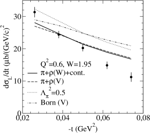
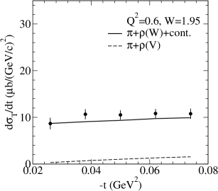
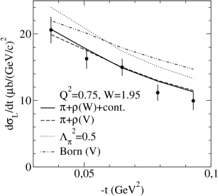
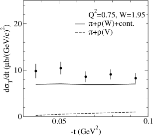
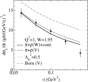
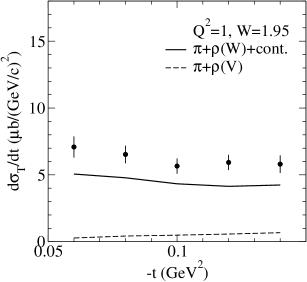
Figure 5: Longitudinal and transverse cross sections for the $p(e,e^{\prime}\pi^{+})n$ reaction at small $Q^{2}\lesssim$ 1 GeV². The unscaled $F\pi 1$ data are centered at $Q^{2}$ of 0.6, 0.75 and 1.GeV². Interference terms between $\pi$-pole, $\rho$-pole and contact $\pi\gamma NN$ amplitudes are taken into account. Results obtained in the $t$-pole approximation with the standard vector (V) $\rho$-meson field are shown by dashed lines. Results for the tensor variant (W) of the $\rho$-meson field (the contact diagram is included) are shown by solid lines (by dotted lines for the fixed value of $\Lambda_{\pi}^{2}=$ 0.5 GeV²/c²). Note that the proper values of $W$ and $Q^{2}$ for each -$t$ bin are different and they differ from the average values shown in the figure legends (see Horn:2006tm ; Tadevosyan:2007yd for detail). For comparison the proper Born approximation results (i.e. without the strong vertex form factors) are shown by double-dot dashed lines.

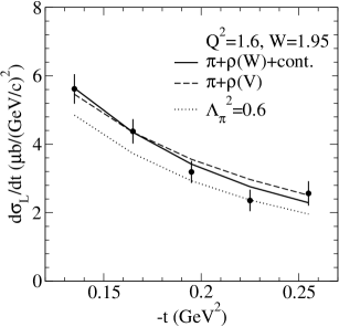
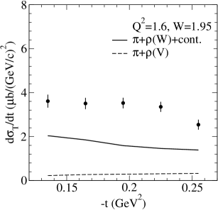
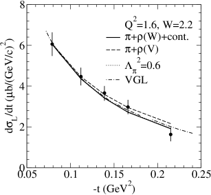
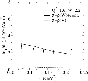
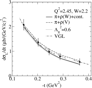
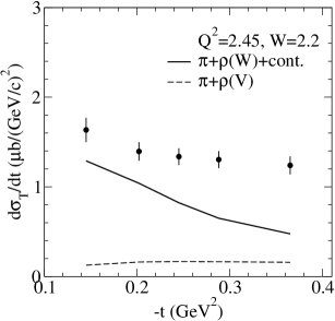
Figure 6: Longitudinal and transverse cross sections at larger values of $Q^{2}$: 1.6 GeV²/c² for the $F\pi$1 data and 1.6 and 2.45 GeV²/c² for the $F\pi$2 data. The same notation as in Fig. 5. The dotted lines correspond to the fixed value of $\Lambda_{\pi}^{2}=$ 0.6 GeV²/c². Here for comparison the VGL model results (adapted from Ref. Horn:2006tm ) are shown by dash-dotted lines.

The approximation (ii) is more realistic. Results of this approximation are displayed in Figs. 5 and 6. By varying the free parameter $Z$ one can obtain a good description of both cross sections $\sigma_{L}$ and $\sigma_{T}$ for the tensor variant of the $\rho$-exchange amplitude ($W$). For the vector variant ($V$) only $\sigma_{L}$ can be described in agreement with experimental data. However, the “soft” variant $(a)$ with $\Lambda_{\rm eff}\approx\Lambda_{\pi}$ used in the form factors $F_{\rho\pi\gamma}(t,Q^{2})$ and $F_{\rm eff}(Q^{2})$ is less suitable for describing the existing data in a large interval of $Q^{2}$ from 0.6 to 2.45 GeV²/c², since it fails to describe the slow $Q^{2}$ dependence of $\sigma_{T}$ in the full interval. The experimental ratio $\sigma_{T}(Q^{2}{=}0.6)/\sigma_{T}(Q^{2}{=}2.45)$ is about 6, while the corresponding ratio of form factors squared $F_{\rho\pi\gamma}^{2}(Q^{2}{=}0.6)/F_{\rho\pi\gamma}^{2}(Q^{2}{=}2.45)$ multiplied by the kinematical factor ${\cal N}_{\sigma}$ (46) is several times larger.

Only the “hard” variant $(b)$ with $\Lambda_{\rm eff}\gtrsim 2\Lambda_{\pi}$ is suitable in describing the data. Taking the value $\Lambda_{\rm eff}=$ 1.2 GeV/c, which is close to the conventional values $\Lambda_{\rho}\approx$ 1 - 1.2 used in literature for the $\rho\pi\gamma$ form factor (see e.g. Horn:2006tm ), and taking the standard “soft” value $\Lambda_{\rm str}^{2}=$ 0.7 GeV²/c² for the common strong form factor (34) we obtain a satisfactory description of both $\sigma_{L}$ and $\sigma_{T}$ cross sections in a wide interval of $Q^{2}$.

The values of the $\rho NN$ coupling constants were fixed to $G_{\rho{\scriptscriptstyle NN}}(0)=$ 4 and $F_{\rho{\scriptscriptstyle NN}}(0)=$ 26 close to the recommended in the ChPT approach Kubis:2000zd of $G_{\rho{\scriptscriptstyle NN}}(0)=$ 4 and $F_{\rho{\scriptscriptstyle NN}}(0)/G_{\rho{\scriptscriptstyle NN}}(0)=$ 6.1 (since the value of $\sigma_{T}$ directly depends on $F_{\rho{\scriptscriptstyle NN}}$ we slightly corrected the conventional value of $F_{\rho{\scriptscriptstyle NN}}(0)$ to obtain the best description of the recent data Horn:2006tm on $\sigma_{T}$ for $Q^{2}=$ 1.6 GeV²/c²). In our calculation we only have one free parameter $Z$ introduced in Eq. (40) as a phenomenological constant, which formally corresponds to a renormalization of the Born contact term $T_{\scriptscriptstyle CPV}$ in the full amplitude (40); in essence the term $ZF_{\rm eff}(Q^{2})F_{\rm str}(t)T_{\scriptscriptstyle CPV}$ amounts to a phenomenological description of the $s$-channel contributions, which otherwise cannot be calculated from first principles. Based on general considerations (see Sect. III) we can only expect that such contributions are suppressed at large $Q^{2}$, and thus a small value of the phenomenological constant $Z$ would be expected.

By varying $Z$ one can improve the description of only one of the cross section component (on account of the another), $\sigma_{L}$ or $\sigma_{T}$. To compare our results to the VGL model predictions Vanderhaeghen:1997ts , which are only realistic for $\sigma_{L}$, we fit the value of $Z$ to the $\sigma_{L}$ data in the full interval 0.6 $<Q^{2}<$ 2.45 GeV²/c². With a value of $Z=$ 0.11 we obtain a description of $\sigma_{L}$ which practically coincides (see Figs. 5 and 6) with the results of the recent Regge-model motivated description of the data Horn:2006tm ; Tadevosyan:2007yd .

The small value of $Z$ correlates well with the quark mechanism proposed in Section IIIB for description of $s$-channel contributions [Figs. 4(b) and 4(c)] to the cross section. In accordance with this picture, only a part of all the possible quark diagrams [Fig. 4(b)] survives at large $Q^{2}$, while the most part of diagrams [of the Fig. 4(c) type] is suppressed because of a high degree $n$ of $\sim Q^{-n}$ behavior (it can be assumed that the value of $Z$ corresponds to the weight $\sim$1/3 of the surviving part of quark diagrams). On the other hand, it would be very difficult to describe this situation at large $Q^{2}$ starting from the interference of many baryon-resonance diagrams depicted in Fig. 2(b). Therefore, the smallness of $Z$ can be considered as an argument in favor of the quark-model motivated representation of the transition amplitude in Eq. (40) and against the naive hadron representation in Eq. (IV).

Following Refs. Horn:2006tm ; Tadevosyan:2007yd , we use different values for the cutoff parameters $\Lambda_{\pi}$ in the $F_{\pi}$ form factor for sets of data centered at different values of $Q^{2}$. In Table 1 we compare the values of $F_{\pi}$ (and correspondingly $\Lambda_{\pi}$) obtained by such a method to the values $F_{\pi}$ obtained in Refs. Horn:2006tm ; Tadevosyan:2007yd on the basis of the VGL model. The coupling constants and cutoff parameters used in the calculation are listed in Table 2.

In the case of the vector variant $V$, which (as is also the case for the VGL model) describes only $\sigma_{L}$ and fails for $\sigma_{T}$, the extracted values of $F_{\pi}$ are close to the results of Refs. Horn:2006tm ; Tadevosyan:2007yd . For the tensor variant $W$ our values for $F_{\pi}$ differ from the ones of Ref. Horn:2006tm ; Tadevosyan:2007yd , but in this case we obtain a satisfactory description of $\sigma_{T}$ as a byproduct of our approach.

It is evident that the proper form factor $F_{\pi}$ cannot fluctuate sharply in magnitude from one $Q^{2}$ to another and the same is true for $\Lambda_{\pi}$ used for its parametrization. However, after smoothing out the fluctuations one can see that there are two $Q^{2}$ regions, $Q^{2}\lesssim$ 1 GeV²/c² and $Q^{2}\gtrsim$ 1 GeV²/c², with different mean values for $\Lambda_{\pi}$. For our $W$ variant we take $\Lambda_{\pi}^{2}=$ 0.5 GeV²/c² in the region of smaller $Q^{2}\leq$ 1 GeV²/c² and $\Lambda_{\pi}^{2}=$ 0.6 GeV²/c² in the $Q^{2}$ region of the recent JLab experiment (in this case in the full interval the mean value of $\Lambda_{\pi}^{2}$ is about 0.54 GeV²/c²) and recalculate the cross section $\sigma_{L}$ (in practice $\sigma_{T}$ does not depend on small $F_{\pi}$ variations). The dotted lines in Figs. 5 and 6 show how $\sigma_{L}(W)$ behaves for these averaged values of $F_{\pi}$. For comparison, the predicted values of $\Lambda_{\pi}^{2}$ for a variety of theoretical approaches are shown in Table 3.

V Summary and conclusions

We analyzed pion electroproduction $p(e,e^{\prime}\pi^{+})n$, which was intensively studied at JLab in the quasi-elastic regime Volmer:2000ek ; Huber:2003kg ; Horn:2006tm ; Tadevosyan:2007yd for the original purpose of directly measuring the pion charge form factor $F_{\pi}(Q^{2})$. Our framework is based on an effective Lagrangian approach involving nucleon, pion, $\rho$ meson and photon degrees of freedom. In the description of the $\rho$ meson we test two possibilities: the so-called vector ($V$) and tensor ($W$) variants. For the standard vector variant $V$ the transverse part $\sigma_{T}$ of the cross section is considerably underestimated, whether it is the Regge model motivated approach VGL Vanderhaeghen:1997ts or the traditional Born one Gutbrod:1973qr modified by strong form factors and contact terms Neudatchin:2004pu ; Obukhovsky:2005sa . Here we have shown that the problem of underestimating $\sigma_{T}$ might be solved by taking into account specific contact terms in the $\rho$ meson propagator that can be most naturally obtained in terms of the tensor variant $W$ of the $\rho$ meson description Ecker:1988te ; Kubis:2000zd .

Based on these findings the uniqueness of the $F_{\pi}$ data extracted from the $\sigma_{L}$ cross section appears doubtful without taking into account the associated data on $\sigma_{T}$. The modified Born approach presented here is successful in the description of both the $\sigma_{L}$ and $\sigma_{T}$ cross sections, thus present a new possibility for the discussion of this problem.

First it should be noted that our results obtained for the standard variant $V$ (the dashed lines in Figs. 5 and 6 for $d\sigma_{L}/dt$) obviously contradict the claim that the Born (i.e. the Feynman tree diagrams) approach is completely unsuited for the description of the forward pion electroproduction process. In our opinion a refined version of this statement would be more adequate: the Born approach is only unsuited for the photoproduction ($Q^{2}=$ 0) and for the low $Q^{2}$ region of electroproduction, but at intermediate and high $Q^{2}$ this approach becomes suitable. This statement is substantiated by a series of previous works Neudatchin:2004pu ; Obukhovsky:2005sa ; Yudin:1998bz ; Neudatchin:2001ex and in particular, by the present detailed evaluation. It seems likely that with growing $Q^{2}$ the full sum (not the isolated terms) of $s(u)$-channel contributions is decreasing most and while the $t$-pole contributions remain. However, any description of such $Q^{2}$ behavior in terms of many baryon poles would be rather complicated and, as a result, very doubtful. We can only use physical arguments based on the comparison of $d\sigma_{L}/dt$ data to the respective $t$-pole contributions depicted in Figs. 5 and 6 for variant $V$ (the dashed line). One can see that starting at $Q^{2}=$ 0.75 GeV²/c² the $t$ behavior of the measured $d\sigma_{L}/dt$ is in a good agreement with predictions given by the $t$-pole contributions (but the agreement breaks down for $Q^{2}=$ 0.6 GeV²/c² and for smaller $Q^{2}$ as our evaluation shows).

Second, the present successful description of $\sigma_{T}$ on the basis of the tensor variant $W$ raises another issue that finally remains to be resolved. Namely, for the variant $V$, which is very similar in results to the VGL model predictions, there is no $\pi$-$\rho$ interference contribution to $\sigma_{L}$ since the corresponding spin average term vanishes (see Appendices). But in the more realistic variant $W$ this term does not vanish and cannot be neglected. In other words, in a realistic variant of the description of both $\sigma_{L}$ and $\sigma_{T}$ the $\rho$-exchange term influences not only $\sigma_{T}$ but $\sigma_{L}$ as well. Hence, the procedure of extracting $F_{\pi}$ values from the $\sigma_{L}$ data alone can, in principle, not be independent from a parallel description of the $\sigma_{T}$ data. We evaluated such a possible indirect influence of the $\sigma_{T}$ data on the final $F_{\pi}$ values extracted from the recent JLab data (see last two rows in Table 1). In our simplified model for the $W$ variant, including a phenomenological contact term (proportional to the free parameter $Z$), we obtained values for $F_{\pi}$ which differ from previous ones (extracted without taking into account the $\sigma_{T}$ data) by about 10 - 15% at $Q^{2}\gtrsim$ 1.6 GeV²/c². This deviation is traced to the $\rho$ - $\pi$ interference, which cannot be neglected. It counts rather in favor of the value $\Lambda_{\pi}^{2}\approx$ 0.6 GeV²/c² obtained in our approach than in favor of the value $\Lambda_{\pi}^{2}\approx$ 0.5 GeV²/c² obtained on the basis of the VGL model. However, now we cannot obtain trustworthy values for the uncertainties $\pm\Delta\Lambda_{\pi}^{2}$ because of the considerable model dependence of the $s$-channel contributions to $\sigma_{L}$.

In future we intent to extend our formalism to the study of kaon electroproduction in connection with the recent JLAB experiment E93-018 Mohring:2002tr .

Appendix A Longitudinal (L) and transverse (T) cross sections

We consider the cross sections $d\sigma_{L,\,T}/dt$ integrated over the azimuthal angle of the emitted pion $\phi_{\pi^{\prime}}^{\ast}$

$$\frac{d\sigma_{L}}{dt} = \int_{0}^{2\pi}\frac{d\sigma_{L}}{dtd\phi_{\pi^{\prime}}^{\ast}}d\phi_{\pi^{\prime}}^{\ast}$$ (48)

$$= \frac{2\pi}{2|{\bf q}^{\ast}||{\bf q}_{r}^{\ast}|}\,\frac{1}{(8\pi W)^{2}}\frac{Q^{2}}{{\bf q}^{2}}\,\overline{J_{0}J_{0}^{\dagger}},$$

$$\frac{d\sigma_{T}}{dt} = \int_{0}^{2\pi}\frac{d\sigma_{T}}{dtd\phi_{\pi^{\prime}}^{\ast}}\,d\phi_{\pi^{\prime}}^{\ast}$$ (49)

$$= \frac{2\pi}{2|{\bf q}^{\ast}||{\bf q}_{r}^{\ast}|}\,\frac{1}{(8\pi W)^{2}}\,\overline{\left(\frac{J_{x}J_{x}^{\dagger}\!+\!J_{y}J_{y}^{\dagger}}{2}\right)}\,.$$

For the cross sections $d\sigma_{TT}/dtd\phi_{\pi^{\prime}}^{\ast}$ and $d\sigma_{LT}/dtd\phi_{\pi^{\prime}}^{\ast}$, which are proportional to $\cos 2\phi_{\pi^{\prime}}^{\ast}$ and $\cos\phi_{\pi^{\prime}}^{\ast}$ respectively, the integral vanishes, and thus the corresponding $d\sigma_{TT,LT}/dt$ values are defined through $d\sigma_{TT,LT}/dtd\phi_{\pi^{\prime}}^{\ast}$ at a fixed angle $\phi_{\pi^{\prime}}^{\ast}=$ 0 times 2$\pi$ in analogy to Eq. (49):

$$\frac{d\sigma_{TT}}{dt}=\left.2\pi\frac{d\sigma_{TT}}{dtd\phi_{\pi^{\prime}}^{\ast}}\right|_{\phi_{\pi^{\prime}}^{a}st\!=0}\\ =\frac{2\pi}{2|{\bf q}^{\ast}||{\bf q}_{r}^{\ast}|}\,\frac{1}{(8\pi W)^{2}}\,\overline{\left(\frac{J_{x}J_{x}^{\dagger}\!-\!J_{y}J_{y}^{\dagger}}{2}\right)}_{\phi_{\pi^{\prime}}^{\ast}\!=0},$$ (50)

$$\frac{d\sigma_{LT}}{dt}=\left.2\pi\frac{d\sigma_{LT}}{dtd\phi_{\pi^{\prime}}^{\ast}}\right|_{\phi_{\pi^{\prime}}^{\ast}\!=0}\\ =\frac{2\pi}{2|{\bf q}^{\ast}||{\bf q}_{r}^{\ast}|}\,\frac{1}{(8\pi W)^{2}}\,\frac{Q}{|{\bf q}|}\,\overline{\left(-\,\frac{J_{0}J_{x}^{\dagger}\!+\!J_{x}J_{0}^{\dagger}}{2}\right)}_{\phi_{\pi^{\prime}}^{\ast}\!=0}\,,$$ (51)

The hadron current tensor $J_{\mu}J_{\nu}$ averaged and summed over nucleon spin projections $s,\,s^{\prime}$

$$\overline{J_{\mu}J_{\nu}^{\dagger}}=\frac{1}{2}\sum_{s,s^{\prime}}\langle p^{\prime},s^{\prime}|J_{\mu}|p,s\rangle\,[\langle p^{\prime},s^{\prime}|J_{\nu}|p,s\rangle]^{\ast}$$ (52)

can be calculated on the basis of the Feynman matrix elements (22), (18), (28) and (30) [see, e.g., Eq. (IV)] which describe the $\pi$-, $\rho$-, nucleon-poles- and contact-term contributions to the hadron current

It is important that the Decart (non-invariant) components of the hadron tensor, $J_{x}J_{x}^{\dagger}$, $J_{0}J_{x}^{\dagger}$, etc., are presented in Eqs. (48) – (51) in a special coordinate frame with the axes $z$ and $y$ directed along the momenta ${\bf q}$ and ${\bf q}\times{\bf k}^{\prime}$, respectively. Any boost along the $z$-axis does not affect the $x$- and $y$-components of the current and, as a result, the transverse components of the hadron tensor become invariant with respect to a change of the reference frame (e.g., from the c.m. system to the lab. system) with

$$\frac{J_{x}J_{x}^{\dagger}\pm J_{y}J_{y}^{\dagger}}{2}=\frac{(J_{x}J_{x}^{\dagger})^{\ast}\pm(J_{y}J_{y}^{\dagger})^{\ast}}{2}\,.$$ (53)

Moreover, in the given coordinate frame $\{xyz\}$ there are further invariants:

$$\frac{Q^{2}}{{\bf q}^{2}}\,J_{0}J_{0}^{\dagger}=\frac{Q^{2}}{{{\bf q}^{\ast}}^{2}}\,(J_{0}J_{0}^{\dagger})^{\ast}\,,$$

$$\frac{Q}{|{\bf q}|}\,[J_{0}J_{x}^{\dagger}+J_{x}J_{0}^{\dagger}]=\frac{Q}{|{\bf q}^{\ast}|}\,[(J_{0}J_{x}^{\dagger})^{\ast}+(J_{x}J_{0}^{\dagger})^{\ast}]\,.$$ (54)

Using the equation

$$\frac{Q}{|{\bf q}|}J_{0}=J^{\mu}\epsilon_{\mu}^{(\lambda\!=0)}(q)\,,$$ (55)

which is valid for a conserved current ($q_{\mu}J^{\mu}=$ 0) one can write the following invariant expressions for all the components of the hadron tensor of interest:

$$\frac{Q^{2}}{{\bf q}^{2}}J_{0}J_{0}^{\dagger}=J^{\mu}\epsilon_{\mu}^{(\lambda\!=0)}\,[J^{\nu}\epsilon_{\nu}^{(\lambda\!=0)}]^{\dagger}\,,$$

$$\frac{J_{x}J_{x}^{\dagger}\pm J_{y}J_{y}^{\dagger}}{2}=\pm\frac{1}{2}\sum_{\lambda\!=\pm 1}J^{\mu}\epsilon_{\mu}^{(\lambda)}\,[J^{\nu}\epsilon_{\nu}^{(\pm\lambda)}]^{\dagger}\,,$$

$$\frac{Q}{|{\bf q}|}\biggl{(}\frac{J_{0}J_{x}^{\dagger}\!+\!J_{x}J_{0}^{\dagger}}{2}\biggr{)}=$$

$$- \frac{1}{2}\sum_{\lambda\!=\pm 1}\frac{\lambda}{\sqrt{2}}\biggl{\{}J^{\mu}\epsilon_{\mu}^{(0)}\,[J^{\nu}\epsilon_{\nu}^{(\lambda)}]^{\dagger}+J^{\mu}\epsilon_{\mu}^{(\lambda)}\,[J^{\nu}\epsilon_{\nu}^{(0)}]^{\dagger}\biggr{\}}\,.$$

Eqs. (44) - (46) of Section IV give the final expressions for the longitudinal and transverse cross sections in the approximation of the lowest order $t-$, $s-$ and $u-$channel diagrams (IV). The sum over spin projections (47) calculated by the standard trace technique results in an universal formula for all the cross sections listed in Eq. (44). Each cross section is expressed through individual dynamical factors $\Phi^{\Gamma,\Gamma^{\prime}}_{pp}(t,Q,W)$, $\Phi^{\Gamma,\Gamma^{\prime}}_{pk}(t,Q,W),\dots$ etc. dependent only on the invariants $t$, $Q^{2}$, $s(=W^{2})$ and the polarization factors $(p\cdot\epsilon^{(\lambda)})$, $(k\cdot\epsilon^{(\lambda)})$, $(\epsilon^{(\lambda)}\cdot{\epsilon^{(\lambda)}}^{\ast})$ common to all the cross sections. This can be illustrated for the example of $d\sigma_{T}/dt$. The transverse cross section is decomposed into a sum of partial ones

$$\frac{d\sigma_{T}}{dt}=\sum_{\scriptscriptstyle\Gamma\Gamma^{\prime}}\frac{d\sigma_{T}^{\scriptscriptstyle\Gamma,\Gamma^{\prime}}}{dt}\,,\ \frac{d\sigma_{T}^{\scriptscriptstyle\Gamma,\Gamma^{\prime}}}{dt}=\frac{1}{2}\sum_{\lambda\!=\!\pm 1}\frac{{\cal N}_{\sigma}}{4\pi}\overline{T_{\scriptscriptstyle\Gamma}(\lambda)T_{\scriptscriptstyle\Gamma^{\prime}}(\lambda)^{\ast}}$$ (57)

where $\Gamma,\Gamma^{\prime}=\pi,\,\rho$, $N(s+u)$, $CPV$ refers to the respective components $T_{\scriptscriptstyle\Gamma}$ and $T^{\ast}_{{\scriptscriptstyle\Gamma}^{\prime}}$ of the full amplitude (IV) taken for calculation of the given partial cross section $d\sigma_{T}^{\scriptscriptstyle\Gamma,\Gamma^{\prime}}/dt$. For $\Gamma=\Gamma^{\prime}$ one obtains the diagonal contribution of the given mechanism “$\Gamma$” to the cross section, while in the case of $\Gamma\neq\Gamma^{\prime}$ the partial cross section $d\sigma_{T}^{\Gamma,\Gamma^{\prime}}/dt$ corresponds to the interference of the amplitudes $T_{\Gamma}$ and $T_{\Gamma^{\prime}}$. The representation of the final result is of the form

$$\frac{d\sigma_{\scriptscriptstyle T}}{dt}=\frac{1}{2}\sum_{\lambda\!=\!\pm 1}\sum_{\Gamma\Gamma^{\prime}}\biggl{\{}(p\cdot\epsilon^{(\lambda)})(p\cdot\epsilon^{(\lambda)\ast})\Phi^{\Gamma,\Gamma^{\prime}}_{pp}\\ +\biggl{[}(p\cdot\epsilon^{(\lambda)})(k\cdot\epsilon^{(\lambda)\ast})+(p\cdot\epsilon^{(\lambda)\ast})(k\cdot\epsilon^{(\lambda)})\biggr{]}\Phi^{\Gamma,\Gamma^{\prime}}_{pk}\\ +(k\cdot\epsilon^{(\lambda)})(k\cdot\epsilon^{(\lambda)\ast})\Phi^{\Gamma,\Gamma^{\prime}}_{kk}+(\epsilon^{(\lambda)}\cdot\epsilon^{(\lambda)\ast})\Phi^{\Gamma,\Gamma^{\prime}}_{ee}\biggr{\}}\,,$$ (58)

$$\frac{d\sigma_{\scriptscriptstyle L}}{dt}=\sum_{\Gamma\Gamma^{\prime}}\biggl{\{}(p\cdot\epsilon^{(0)})(p\cdot\epsilon^{(0)\ast})\Phi^{\Gamma,\Gamma^{\prime}}_{pp}\\ +\biggl{[}(p\cdot\epsilon^{(0)})(k\cdot\epsilon^{(0)\ast})+(p\cdot\epsilon^{(0)\ast})(k\cdot\epsilon^{(0)})\biggr{]}\Phi^{\Gamma,\Gamma^{\prime}}_{pk}\\ +(k\cdot\epsilon^{(0)})(k\cdot\epsilon^{(0)\ast})\Phi^{\Gamma,\Gamma^{\prime}}_{kk}+(\epsilon^{(\lambda)}\cdot\epsilon^{(0)\ast})\Phi^{\Gamma,\Gamma^{\prime}}_{ee}\biggr{\}}\,,$$ (59)

containing separately the polarization components $(\kappa\cdot\epsilon^{(\lambda)}(q))(\kappa^{\prime}\cdot\epsilon^{(\lambda)\ast}(q))$ and the dynamical ones $\Phi^{\Gamma,\Gamma^{\prime}}_{\kappa\kappa^{\prime}}$. In Appendices B, C and D we list the full analytical results for both $\sigma_{L}$ and $\sigma_{T}$ parts given for all the diagonal and interference terms.

Appendix B Polarization factors

To further symplify formulas some new dimensionless, invariant variables are specified,

$$\eta=\frac{-t}{4m_{\scriptscriptstyle N}^{2}},\quad\xi_{s}\equiv\frac{p\cdot q}{m_{\scriptscriptstyle N}Q}=\frac{Q^{2}+W^{2}-m_{\scriptscriptstyle N}^{2}}{2m_{\scriptscriptstyle N}Q},\quad\xi_{t}\equiv\frac{k\cdot q}{m_{\scriptscriptstyle N}Q}=\frac{Q^{2}-t+M_{\pi}^{2}}{2m_{\scriptscriptstyle N}Q}.$$ (60)

Longitudinal factors :

$$(p\cdot\epsilon^{(\lambda\!=\!0)})(p\cdot\epsilon^{(\lambda\!=\!0)\,\ast})_{\rm lab}=m_{\scriptscriptstyle N}^{2}(1+\xi_{s}^{2}),\quad(k\cdot\epsilon^{(\lambda\!=\!0)})(k\cdot\epsilon^{(\lambda\!=\!0)\,\ast})_{\rm lab}=\frac{m_{\scriptscriptstyle N}^{2}}{1+\xi_{s}^{2}}(-2\eta+\xi_{s}\xi_{t})^{2},$$

$$\left[(p\cdot\epsilon^{(\lambda\!=\!0)})(k\cdot\epsilon^{(\lambda\!=\!0)\,\ast})+(p\cdot\epsilon^{(\lambda\!=\!0)\,\ast})(k\cdot\epsilon^{(\lambda\!=\!0)})\right]_{\rm lab}=2m_{\scriptscriptstyle N}^{2}(-2\eta+\xi_{s}\xi_{t})\,,$$

$$(\epsilon^{(\lambda\!=\!0)}\cdot\epsilon^{(\lambda\!=\!0)})=1\,.$$ (61)

Transverse factors:

$$\frac{1}{2}\sum_{\lambda=\pm 1}(p\cdot\epsilon^{(\lambda)})(p\cdot\epsilon^{(\lambda)\,\ast})_{\rm lab}=0\,,\quad\frac{1}{2}\sum_{\lambda=\pm 1}\left[(p\cdot\epsilon^{(\lambda)})(k\cdot\epsilon^{(\lambda)\,\ast})+(p\cdot\epsilon^{(\lambda)\,\ast})(k\cdot\epsilon^{(\lambda)})\right]_{\rm lab}=0\,,$$

$$\frac{1}{2}\sum_{\lambda=\pm 1}(k\cdot\epsilon^{(\lambda)})(k\cdot\epsilon^{(\lambda)\,\ast})_{\rm lab}=\frac{-t}{2(1+\xi_{s}^{2})}(1+\eta+\xi_{s}^{2}+\xi_{t}^{2}-\xi_{s}\xi_{t})=\frac{1}{2}{\bf k}_{\rm lab}^{2}\,\sin^{2}\theta_{k}^{\rm lab},$$

$$\frac{1}{2}\sum_{\lambda=\pm 1}(\epsilon^{(\lambda)}\cdot\epsilon^{(\lambda)\,\ast})=-1\,.$$ (62)

Here $\theta_{k}^{\rm lab}$ is the angle between the vectors ${\bf k}$ and ${\bf q}$ in the lab. frame:

$$|{\bf k}_{\rm lab}|\cos\theta_{k}^{\rm lab}=\frac{m_{\scriptscriptstyle N}}{\sqrt{1+\xi_{s}^{2}}}(-2\eta\xi_{s}-\xi_{t})\,,\qquad|{\bf k}_{\rm lab}|\equiv|{\bf k}|=\sqrt{-t\left(1-\frac{t}{4m_{\scriptscriptstyle N}^{2}}\right)}.$$ (63)

Appendix C Diagonal contributions to the cross section

C.1 The diagonal ${\pi}$-meson $t$-pole part

$$\frac{1}{4\pi}\overline{|T_{\pi}(\lambda)|^{2}} = 8\alpha F_{\pi}^{2}(Q^{2})\frac{g_{\pi{\scriptscriptstyle NN}}^{2}(t)}{(M_{\pi}^{2}-t)^{2}}\biggl{\{}(p\cdot\epsilon^{(\lambda)})(p\cdot\epsilon^{(\lambda)\,\ast})P_{pp}+(k\cdot\epsilon^{(\lambda)})(k\cdot\epsilon^{(\lambda)\,\ast})P_{kk}$$ (64)

$$+ \left[(p\cdot\epsilon^{(\lambda)})(k\cdot\epsilon^{(\lambda)\,\ast})+(p\cdot\epsilon^{(\lambda)\,\ast})(k\cdot\epsilon^{(\lambda)})\right]P_{pk}+(\epsilon^{(\lambda)}\cdot\epsilon^{(\lambda)\,\ast})P_{ee}\biggr{\}}\,,$$

Invariant factors $P_{\kappa\kappa^{\prime}}\,(\equiv\Phi^{\pi\pi}_{\kappa\kappa^{\prime}}(t,Q,W)\,)$ are the same for PS and PV couplings:

$$P_{kk}=-t,\qquad P_{pp}=P_{pk}=P_{ee}=0\,.$$ (65)

C.2 The diagonal ${\rho}$-meson $t$-pole part

$$\frac{1}{4\pi}\overline{|T_{\rho}^{V(W)}(\lambda)|^{2}} = \frac{\alpha}{2}\frac{g_{\rho\pi\gamma}^{2}(t,Q^{2})}{(M_{\rho}^{2}-t)^{2}}m_{\scriptscriptstyle N}^{2}\biggl{\{}(p\cdot\epsilon^{(\lambda)})(p\cdot\epsilon^{(\lambda)\,\ast})R_{pp}^{V(W)}+(k\cdot\epsilon^{(\lambda)})(k\cdot\epsilon^{(\lambda)\,\ast})R_{kk}^{V(W)}$$ (66)

$$+ \biggl{[}(p\cdot\epsilon^{(\lambda)})(k\cdot\epsilon^{(\lambda)\,\ast})+(p\cdot\epsilon^{(\lambda)\,\ast})(k\cdot\epsilon^{(\lambda)})\biggr{]}R_{pk}^{V(W)}+(\epsilon^{(\lambda)}\cdot\epsilon^{(\lambda)\,\ast})R_{ee}^{V(W)}\biggr{\}}\,.$$

Invariant factors $R^{V(W)}_{\kappa\kappa^{\prime}}\,(\equiv\Phi^{\rho\rho}_{\kappa\kappa^{\prime}}(t,Q,W)\,)$:

$$R_{pp}^{V} = 4Q^{2}\biggl{[}-(\xi_{t}^{2}-4\eta)\biggl{(}G_{\rho}^{2}+\eta F_{\rho}^{2}\biggr{)}\biggr{]}\,,$$ (67)

$$R_{pp}^{W} = R_{pp}^{V}+4Q^{2}\biggl{(}\frac{M_{\rho}^{2}-t}{m_{\scriptscriptstyle N}^{2}}\biggr{)}\biggl{(}\frac{1}{2}\xi_{t}^{2}+\frac{M_{\rho}^{2}+t}{4m_{\scriptscriptstyle N}^{2}}\biggr{)}F_{\rho}^{2}\,,$$ (68)

$$R_{pk}^{V} = 4Q^{2}\biggl{[}(\xi_{s}\xi_{t}-2\eta)\biggl{(}G_{\rho}^{2}+\eta F_{\rho}^{2}\biggr{)}\biggr{]}\,,$$ (69)

$$R_{pk}^{W} = R_{pk}^{\mbox{v}}+4Q^{2}\biggl{(}\frac{M_{\rho}^{2}-t}{m_{\scriptscriptstyle N}^{2}}\biggr{)}\biggl{[}-\frac{1}{2}\biggl{(}\xi_{s}\xi_{t}+\frac{M_{\rho}^{2}+t}{4m_{\scriptscriptstyle N}^{2}}\biggr{)}\biggr{]}F_{\rho}^{2}\,,$$ (70)

$$R_{kk}^{V} = 4Q^{2}\biggl{[}-\xi_{s}^{2}\biggl{(}G_{\rho}^{2}+\eta F_{\rho}^{2}\biggr{)}+2\eta G_{\rho}F_{\rho}-(1-\eta)G_{\rho}^{2}\biggr{]}\,,$$ (71)

$$R_{kk}^{W} = R_{kk}^{\mbox{v}}+4Q^{2}\biggl{(}\frac{M_{\rho}^{2}-t}{m_{\scriptscriptstyle N}^{2}}\biggr{)}\biggl{[}\frac{1}{2}(\xi_{s}^{2}F_{\rho}^{2}-G_{\rho}F_{\rho})\biggr{]}\,,$$ (72)

$$R_{ee}^{V} = 4Q^{2}m_{\scriptscriptstyle N}^{2}\biggl{\{}\biggl{[}\xi_{t}^{2}-4\eta\xi_{s}(\xi_{s}-\xi_{t})\biggr{]}\biggl{(}G_{\rho}^{2}+\eta F_{\rho}^{2}\biggr{)}-\eta\xi_{t}^{2}(G_{\rho}+F_{\rho})^{2}-4\eta(G_{\rho}-\eta F_{\rho})^{2}\biggr{\}}\,,$$ (73)

$$R_{ee}^{W} = R_{ee}^{V}+4Q^{2}m_{\scriptscriptstyle N}^{2}\biggl{(}\frac{M_{\rho}^{2}-t}{m_{\scriptscriptstyle N}^{2}}\biggr{)}\biggl{\{}-\,\frac{M_{\rho}^{2}+t}{4m_{\scriptscriptstyle N}^{2}}\biggl{[}\xi_{s}(\xi_{s}-\xi_{t})+\eta\biggr{]}F_{\rho}^{2}+\frac{1}{2}(\xi_{t}^{2}-4\eta)G_{\rho}F_{\rho}\biggr{\}}\,.$$ (74)

Here for simplicity we define $G_{\rho}=G_{\rho NN}(t)$ and $F_{\rho}=F_{\rho NN}(t)$.

C.3 The diagonal nucleon ($s$- and $u$-pole) part

$$\frac{1}{4\pi}\overline{|T_{{\scriptscriptstyle N}(s+u)}(\lambda)|^{2}} = 2\alpha\frac{g_{\pi{\scriptscriptstyle NN}}^{2}F_{\rm eff}^{2}(t,Q^{2})}{(W^{2}-m_{\scriptscriptstyle N}^{2})^{2}}\biggl{\{}(p\cdot\epsilon^{(\lambda)})(p\cdot\epsilon^{(\lambda)\,\ast})U_{pp}+(k\cdot\epsilon^{(\lambda)})(k\cdot\epsilon^{(\lambda)\,\ast})U_{kk}$$ (75)

$$+ \biggl{[}(p\cdot\epsilon^{(\lambda)})(k\cdot\epsilon^{(\lambda)\,\ast})+(p\cdot\epsilon^{(\lambda)\,\ast})(k\cdot\epsilon^{(\lambda)})\biggr{]}U_{pk}+(\epsilon^{(\lambda)}\cdot\epsilon^{(\lambda)\,\ast})U_{ee}\biggr{\}}\,.$$

Invariant factors $U_{\kappa\kappa^{\prime}}\,(\,\equiv\Phi^{\scriptscriptstyle NN}_{\kappa\kappa^{\prime}}(t,Q,W)\,)$:

$$U_{pp} = 4m_{\scriptscriptstyle N}^{2}\biggl{\{}-\frac{M_{\pi}^{2}}{m_{\scriptscriptstyle N}^{2}}\biggr{[}(F_{1p}-\widetilde{F}_{1n})^{2}+\frac{Q^{2}}{4m_{\scriptscriptstyle N}^{2}}(F_{2p}-\widetilde{F}_{2n})^{2}\biggr{]}+\frac{Q^{2}}{m_{\scriptscriptstyle N}^{2}}\biggl{(}\xi_{t}-\frac{Q}{m_{\scriptscriptstyle N}}\biggr{)}^{2}F_{2p}\widetilde{F}_{2n}\biggr{\}}\,,$$ (76)

$$U_{pk} = 4m_{\scriptscriptstyle N}^{2}\biggl{\{}\frac{Q}{m_{\scriptscriptstyle N}}\biggl{(}\xi_{s}-\frac{Q}{2m_{\scriptscriptstyle N}}\biggr{)}\biggl{[}(F_{1p}-\widetilde{F}_{1n})^{2}+\frac{Q^{2}}{4m_{\scriptscriptstyle N}^{2}}(F_{2p}-\widetilde{F}_{2n})^{2}-\frac{Q}{m_{\scriptscriptstyle N}}\biggl{(}\xi_{t}-\frac{Q}{m_{\scriptscriptstyle N}}\biggr{)}F_{2p}\widetilde{F}_{2n}\biggr{]}$$ (77)

$$- \biggl{(}\frac{Q}{m_{\scriptscriptstyle N}}\xi_{t}-4\eta\biggr{)}\biggl{[}(F_{1p}-\widetilde{F}_{1n})\widetilde{F}_{1n}+\frac{Q^{2}}{4m_{\scriptscriptstyle N}^{2}}(F_{2p}-\widetilde{F}_{2n})\widetilde{F}_{2n}\biggr{]}\biggr{\}}\,,$$

$$U_{kk} = 4m_{\scriptscriptstyle N}^{2}\biggl{\{}\frac{2Q}{m_{\scriptscriptstyle N}}\xi_{s}\biggl{[}(F_{1p}-\widetilde{F}_{1n})\widetilde{F}_{1n}+\frac{Q^{2}}{4m_{\scriptscriptstyle N}^{2}}(F_{2p}-\widetilde{F}_{2n})\widetilde{F}_{2n}\biggr{]}+4\eta\biggl{(}\widetilde{F}_{1n}^{2}+\frac{Q^{2}}{4m_{\scriptscriptstyle N}^{2}}\widetilde{F}_{2n}^{2}\biggr{)}$$ (78)

$$+ \frac{Q^{2}}{m_{\scriptscriptstyle N}^{2}}\biggr{[}\biggl{(}\xi_{s}^{2}-\frac{Q}{m_{\scriptscriptstyle N}}\xi_{s}+1\biggr{)}F_{2p}\widetilde{F}_{2n}+(F_{1p}\widetilde{F}_{2n}+\widetilde{F}_{1n}F_{2p})\biggr{]}\biggr{\}}\,,$$

$$U_{ee} = 4m_{\scriptscriptstyle N}^{2}Q^{2}\biggl{\{}\biggl{[}\frac{Q}{2m_{\scriptscriptstyle N}}\biggl{(}\xi_{t}-\frac{Q}{2m_{\scriptscriptstyle N}}\biggr{)}-\eta\biggl{(}\xi_{s}-\frac{Q}{2m_{\scriptscriptstyle N}}\biggr{)}^{2}\biggr{]}(F_{2p}-\widetilde{F}_{2n})^{2}$$ (79)

$$+ \xi_{s}(\xi_{t}-\xi_{s})(F_{1p}-\widetilde{F}_{1n})^{2}-\biggl{[}\frac{Q}{2m_{\scriptscriptstyle N}}(2\xi_{s}-\xi_{t})-\xi_{s}\xi_{t}\biggr{]}(F_{1p}-\widetilde{F}_{1n})(F_{2p}-\widetilde{F}_{2n})$$

$$- 2\biggl{[}\frac{Q}{2m_{\scriptscriptstyle N}}(2\xi_{s}-\xi_{t})-\xi_{s}\xi_{t}+\frac{1}{2}\xi_{t}^{2}\biggr{]}\biggl{[}(F_{1p}-\widetilde{F}_{1n})-\eta(F_{2p}-\widetilde{F}_{2n})\biggr{]}\widetilde{F}_{2n}$$

$$- \,(1+\eta)\left(\xi_{t}-\frac{Q}{m_{\scriptscriptstyle N}}\right)^{2}F_{2p}\widetilde{F}_{2n}-\eta(F_{1p}-\widetilde{F}_{1n}+F_{2p}-\widetilde{F}_{2n})^{2}\biggr{\}}\,,$$

where $F_{1p}$, $F_{2p}$, $F_{1n}$ and $F_{2n}$ are the Dirac nucleon form factors and we denote for simplicity

$$\widetilde{F}_{in}=\frac{W^{2}-m_{\scriptscriptstyle N}^{2}}{W^{2}-m_{\scriptscriptstyle N}^{2}+Q^{2}+t-M_{\pi}^{2}}{F}_{in},\quad F_{ip}=F_{ip}(Q^{2}),\quad F_{in}=F_{in}(Q^{2}),\quad i=1,\,2.$$ (80)

C.4 The diagonal part of the contact term contribution

$$\frac{1}{4\pi}\overline{|T_{\scriptscriptstyle CPV}(\lambda)|^{2}} = \alpha F_{\pi}^{2}(Q^{2})\frac{g_{\pi{\scriptscriptstyle NN}}^{2}(t)}{2m_{\scriptscriptstyle N}^{2}}\biggl{\{}(p\cdot\epsilon^{(\lambda)})(p\cdot\epsilon^{(\lambda)\,\ast})C_{pp}+(k\cdot\epsilon^{(\lambda)})(k\cdot\epsilon^{(\lambda)\,\ast})C_{kk}$$ (81)

$$+ \biggl{[}(p\cdot\epsilon^{(\lambda)})(k\cdot\epsilon^{(\lambda)\,\ast})+(p\cdot\epsilon^{(\lambda)\,\ast})(k\cdot\epsilon^{(\lambda)})\biggr{]}C_{pk}+(\epsilon^{(\lambda)}\cdot\epsilon^{(\lambda)\,\ast})C_{ee}\biggr{\}}$$

Invariant factors $C_{\kappa\kappa^{\prime}}\,(\equiv\Phi^{\pi\gamma{-}\pi\gamma}_{\kappa\kappa^{\prime}}(t,Q,W)\,)$:

$$C_{pp}=4,\qquad C_{pk}=-2,\qquad C_{kk}=0,\qquad C_{ee}=-4m_{\scriptscriptstyle N}^{2}(1+\eta).$$ (82)

Appendix D Interference terms

D.1 Interference terms for the ${\bm{\pi}}$- and ${\bm{\rho}}$-meson poles

$$\frac{1}{4\pi}\overline{\biggl{[}T_{\pi}(\lambda)T_{\rho}^{V(W)\ast}(\lambda)+T_{\rho}^{V(W)}(\lambda)T_{\pi}^{\ast}(\lambda)\biggr{]}}=$$ (83)

$$= \alpha m_{\scriptscriptstyle N}F_{\pi}(Q^{2})\frac{g_{\pi{\scriptscriptstyle NN}}(t)}{M_{\pi}^{2}-t}\frac{g_{\rho\pi\gamma}(t,Q^{2})}{M_{\rho}^{2}-t}\biggl{\{}(p\cdot\epsilon^{(\lambda)})(p\cdot\epsilon^{(\lambda)\,\ast})T_{pp}^{V(W)}+(k\cdot\epsilon^{(\lambda)})(k\cdot\epsilon^{(\lambda)\,\ast})T_{kk}^{V(W)}$$

$$+ \biggl{[}(p\cdot\epsilon^{(\lambda)})(k\cdot\epsilon^{(\lambda)\,\ast})+(p\cdot\epsilon^{(\lambda)\,\ast})(k\cdot\epsilon^{(\lambda)})\biggr{]}T_{pk}^{V(W)}+(\epsilon^{(\lambda)}\cdot\epsilon^{(\lambda)\,\ast})T_{ee}^{V(W)}\biggr{\}}\,.$$

Invariant factors $T^{V(W)}_{\kappa\kappa^{\prime}}\,(\equiv\Phi^{\pi\rho}_{\kappa\kappa^{\prime}}(t,Q,W)\,)$ are the same for PS- and PV couplings:

$$T_{pk}^{W}=-\,2Qm_{\scriptscriptstyle N}\biggl{(}\frac{M_{\rho}^{2}-t}{m_{\scriptscriptstyle N}^{2}}\biggr{)}\xi_{t}F_{\rho}(t)\,,\qquad T_{kk}^{W}=4Qm_{\scriptscriptstyle N}\biggl{(}\frac{M_{\rho}^{2}-t}{m_{\scriptscriptstyle N}^{2}}\biggr{)}\xi_{s}F_{\rho}(t)\,,$$

$$T_{pp}^{V}=T_{pk}^{V}=T_{kk}^{V}=T_{ee}^{V}=0,\hskip 54.06006ptT_{pp}^{W}=T_{ee}^{W}=0\,.$$ (84)

D.2 Interference terms for the ${\bm{\pi}}$-meson ($t$) and nucleon ($s+u$) poles

$$\frac{1}{4\pi}\overline{\biggl{[}T_{\pi}(\lambda)T_{{\scriptscriptstyle N}(s+u)}^{\ast}(\lambda)+T_{{\scriptscriptstyle N}(s+u)}(\lambda)T_{\pi}^{\ast}(\lambda)\biggr{]}}=$$ (85)

$$= -2\alpha F_{\pi}(Q^{2})\frac{g_{\pi{\scriptscriptstyle NN}}(t)}{M_{\pi}^{2}-t}\frac{g_{\pi{\scriptscriptstyle NN}}F_{\rm eff}(t,Q^{2})}{W^{2}-m_{\scriptscriptstyle N}^{2}}\biggl{\{}(p\cdot\epsilon^{(\lambda)})(p\cdot\epsilon^{(\lambda)\,\ast})N_{pp}+(k\cdot\epsilon^{(\lambda)})(k\cdot\epsilon^{(\lambda)\,\ast})N_{kk}$$

$$+ \biggl{[}(p\cdot\epsilon^{(\lambda)})(k\cdot\epsilon^{(\lambda)\,\ast})+(p\cdot\epsilon^{(\lambda)\,\ast})(k\cdot\epsilon^{(\lambda)})\biggr{]}N_{pk}+(\epsilon^{(\lambda)}\cdot\epsilon^{(\lambda)\,\ast})N_{ee}\biggr{\}}$$

Invariant factors $N_{\kappa\kappa^{\prime}}\,(\equiv\Phi^{\pi{\scriptscriptstyle N}}_{\kappa\kappa^{\prime}}(t,Q,W)\,)$ are different for PS and PV couplings

1) PS coupling:

$$N_{pp}=N_{ee}=0\,,\qquad\qquad N_{pk}=-4m_{\scriptscriptstyle N}^{2}\biggl{(}4\eta-\frac{Q}{m_{\scriptscriptstyle N}}\xi_{t}\biggr{)}\biggl{(}F_{1p}-\widetilde{F}_{1n}\biggr{)},$$

$$N_{kk}=-8m_{\scriptscriptstyle N}^{2}\biggl{[}4\eta\widetilde{F}_{1n}+\frac{Q}{m_{\scriptscriptstyle N}}\xi_{s}(F_{1p}-\widetilde{F}_{1n})+\frac{Q^{2}}{2m_{\scriptscriptstyle N}^{2}}(F_{2p}+\widetilde{F}_{2n})\biggr{]}$$ (86)

2) PV coupling:

$$N_{pp} = N_{ee}\,=\,0\,,$$ (87)

$$N_{pk} = -4m_{\scriptscriptstyle N}^{2}\biggl{[}4\eta(F_{1p}-\widetilde{F}_{1n})-\frac{Q}{m_{\scriptscriptstyle N}}\xi_{t}\biggl{(}(F_{1p}-\widetilde{F}_{1n})-\frac{Q^{2}}{4m_{\scriptscriptstyle N}^{2}}(F_{2p}-\widetilde{F}_{2n})\biggr{)}$$ (88)

$$- \frac{Q^{2}}{2m_{\scriptscriptstyle N}^{2}}\xi_{t}\biggl{(}\xi_{s}(F_{2p}+\widetilde{F}_{2n})-\xi_{t}\widetilde{F}_{2n}\biggr{)}\biggr{]}\,,$$

$$N_{kk} = -8m_{\scriptscriptstyle N}^{2}\biggl{[}(4\eta-\frac{Q}{m_{\scriptscriptstyle N}}\xi_{t})\,\widetilde{F}_{1n}-\frac{Q}{m_{\scriptscriptstyle N}}\xi_{s}\frac{Q^{2}}{4m_{\scriptscriptstyle N}^{2}}(F_{2p}-\widetilde{F}_{2n})$$ (89)

$$+ \frac{Q^{2}}{2m_{\scriptscriptstyle N}^{2}}\xi_{s}\biggl{(}\xi_{s}(F_{2p}+\widetilde{F}_{2n})-\xi_{t}\widetilde{F}_{2n}\biggr{)}+\frac{Q^{2}}{2m_{\scriptscriptstyle N}^{2}}(F_{1p}+\widetilde{F}_{1n}+F_{2p}+\widetilde{F}_{2n})\biggr{]}\,.$$

D.3 Interference term for the ${\bm{\pi}}$-meson pole and the contact ${\bm{\gamma}}{\bm{\pi}}{\bf NN}$ vertex

$$\frac{1}{4\pi}\overline{\biggl{[}T_{\pi}(\lambda)T_{\scriptscriptstyle CPV}^{\ast}(\lambda)+T_{\scriptscriptstyle CPV}(\lambda)T_{\pi}^{\ast}(\lambda)\biggr{]}}=$$ (90)

$$= \alpha F_{\pi}^{2}(Q^{2})\frac{g_{\pi{\scriptscriptstyle NN}}^{2}(t)}{2m_{\scriptscriptstyle N}^{2}\,M_{\pi}^{2}-t}\biggl{\{}(p\cdot\epsilon^{(\lambda)})(p\cdot\epsilon^{(\lambda)\,\ast})P_{pp}+\biggl{[}(p\cdot\epsilon^{(\lambda)})(k\cdot\epsilon^{(\lambda)\,\ast})+(p\cdot\epsilon^{(\lambda)\,\ast})(k\cdot\epsilon^{(\lambda)})\biggr{]}P_{pk}$$

$$+ (k\cdot\epsilon^{(\lambda)})(k\cdot\epsilon^{(\lambda)\,\ast})P_{kk}+(\epsilon^{(\lambda)}\cdot\epsilon^{(\lambda)\,\ast})P_{ee}\biggr{\}}$$

Invariant factors $P_{\kappa\kappa^{\prime}}\,(\equiv\Phi^{\pi{-}{\scriptscriptstyle CPV}}_{\kappa\kappa^{\prime}}(t,Q,W)\,)$:

$$P_{pp}=P_{pk}=P_{ee}=0,\qquad P_{kk}=16m_{\scriptscriptstyle N}^{2}\,.$$ (91)

D.4 Interference terms for the ${\bm{\rho}}$-meson ($t$) and nucleon ($s+u$) poles

$$\frac{1}{4\pi}\overline{\biggl{[}T_{{\scriptscriptstyle N}(s+u)}(\lambda)T_{\rho}^{V(W)\ast}(\lambda)+T_{\rho}^{V(W)}(\lambda)T_{{\scriptscriptstyle N}(s+u)}^{\ast}(\lambda)\biggr{]}}=$$ (92)

$$= -\alpha m_{\scriptscriptstyle N}\frac{g_{\rho\pi\gamma}(t,Q^{2})}{M_{\rho}^{2}-t}\frac{g_{\pi{\scriptscriptstyle NN}}F_{\rm eff}(t,Q^{2})}{W^{2}-m_{\scriptscriptstyle N}^{2}}\,\biggl{\{}(p\cdot\epsilon^{(\lambda)})(p\cdot\epsilon^{(\lambda)\,\ast})H_{pp}^{\{\mbox{v,w}\}}+(k\cdot\epsilon^{(\lambda)})(k\cdot\epsilon^{(\lambda)\,\ast})H_{kk}^{V(W)}$$

$$+ \biggl{[}(p\cdot\epsilon^{(\lambda)})(k\cdot\epsilon^{(\lambda)\,\ast})+(p\cdot\epsilon^{(\lambda)\,\ast})(k\cdot\epsilon^{(\lambda)})\biggr{]}H_{pk}^{V(W)}+(\epsilon^{(\lambda)}\cdot\epsilon^{(\lambda)\,\ast})H_{ee}^{V(W)}\biggr{\}}\,.$$

Invariant factors $H^{V(W)}_{\kappa\kappa^{\prime}}\,(\equiv\Phi^{\rho{\scriptscriptstyle N}}_{\kappa\kappa^{\prime}}(t,Q,W)\,)$

1) PS coupling:

$$H_{pp}^{V} = 4Q^{2}(\xi_{t}^{2}-4\eta)\biggl{[}\biggl{(}F_{1p}-\widetilde{F}_{1n}\biggr{)}F_{\rho}-\biggl{(}F_{2p}-\widetilde{F}_{2n}\biggr{)}G_{\rho}\biggr{]}\,,$$ (93)

$$H_{pp}^{W} = H_{pp}^{V}+4Qm_{\scriptscriptstyle N}\biggl{(}\frac{M_{\rho}^{2}-t}{m_{\scriptscriptstyle N}^{2}}\biggr{)}\biggl{(}\frac{Q}{m_{\scriptscriptstyle N}}-\xi_{t}\biggr{)}\biggl{(}F_{1p}-\widetilde{F}_{1n}\biggr{)}F_{\rho}\,,$$ (94)

$$H_{pk}^{V} = 4Q^{2}\biggl{\{}-\xi_{s}\xi_{t}\biggl{[}\biggl{(}F_{1p}-\widetilde{F}_{1n}\biggr{)}F_{\rho}-\biggl{(}F_{2p}-\widetilde{F}_{2n}\biggr{)}G_{\rho}\biggr{]}-\xi_{t}\frac{Q}{4m_{\scriptscriptstyle N}}\biggl{(}F_{2p}+\widetilde{F}_{2n}\biggr{)}(G_{\rho}+F_{\rho})$$ (95)

$$+ \eta\biggl{[}\biggl{(}F_{2p}-\widetilde{F}_{2n}\biggr{)}(F_{\rho}-G_{\rho})+2\biggl{(}F_{1p}-\widetilde{F}_{1n}\biggr{)}F_{\rho}+2\widetilde{F}_{2n}(G_{\rho}+F_{\rho})\biggr{]}\biggr{\}}\,,$$

$$H_{pk}^{W} = H_{pk}^{V}+4Qm_{\scriptscriptstyle N}\biggl{(}\frac{M_{\rho}^{2}-t}{m_{\scriptscriptstyle N}^{2}}\biggr{)}\biggl{[}\biggl{(}\frac{1}{2}\xi_{s}-\frac{Q}{2m_{\scriptscriptstyle N}}\biggr{)}\biggl{(}F_{1p}-\widetilde{F}_{1n}\biggr{)}-\frac{1}{2}\xi_{t}\widetilde{F}_{1n}-\frac{Q}{4m_{\scriptscriptstyle N}}\biggl{(}F_{2p}+\widetilde{F}_{2n}\biggr{)}\biggr{]}F_{\rho}\,,$$ (96)

$$H_{kk}^{V} = 4Q^{2}\biggl{[}\biggl{(}F_{1p}-\widetilde{F}_{1n}\biggr{)}\biggl{(}\xi_{s}^{2}F_{\rho}-G_{\rho}\biggr{)}-\biggl{(}1+\xi_{s}^{2}\biggr{)}\biggl{(}F_{2p}-\widetilde{F}_{2n}\biggr{)}G_{\rho}$$ (97)

$$+ \xi_{s}\frac{Q}{2m_{\scriptscriptstyle N}}\biggl{(}F_{2p}+\widetilde{F}_{2n}\biggr{)}(G_{\rho}+F_{\rho})-2\eta\widetilde{F}_{2n}(G_{\rho}+F_{\rho})\biggr{]}\,,$$

$$H_{kk}^{W} = H_{kk}^{\mbox{v}}+4Qm_{\scriptscriptstyle N}\biggl{(}\frac{M_{\rho}^{2}-t}{m_{\scriptscriptstyle N}^{2}}\biggr{)}\biggl{(}\xi_{s}\widetilde{F}_{1n}+\frac{Q}{2m_{\scriptscriptstyle N}}\widetilde{F}_{2n}\biggr{)}F_{\rho}\,,$$ (98)

$$H_{ee}^{V} = 4Q^{2}m_{\scriptscriptstyle N}^{2}\biggl{\{}\eta\biggl{[}\biggl{(}\xi_{t}-2\xi_{s}\biggr{)}\biggl{(}\xi_{t}-\frac{Q}{m_{\scriptscriptstyle N}}\biggr{)}\biggl{(}F_{2p}+\widetilde{F}_{2n}\biggr{)}(G_{\rho}+F_{\rho})-\xi_{t}^{2}\biggl{(}F_{2p}-\widetilde{F}_{2n}\biggr{)}(G_{\rho}+F_{\rho})$$ (99)

$$+ 4\xi_{s}\biggl{(}\xi_{s}-\xi_{t}\biggr{)}\biggl{(}(F_{1p}-\widetilde{F}_{1n})F_{\rho}-(F_{2p}-\widetilde{F}_{2n})G_{\rho}\biggr{)}-4(F_{1p}-\widetilde{F}_{1n}+F_{2p}-\widetilde{F}_{2n})(G_{\rho}-\eta F_{\rho})\biggr{]}$$

$$+ \xi_{t}^{2}(F_{1p}-\widetilde{F}_{1n}+F_{2p}-\widetilde{F}_{2n})G_{\rho}\biggr{\}}\,,$$

$$H_{ee}^{W} = H_{ee}^{\mbox{v}}+4Q^{2}m_{\scriptscriptstyle N}^{2}\biggl{(}\frac{M_{\rho}^{2}-t}{m_{\scriptscriptstyle N}^{2}}\biggr{)}\biggl{\{}\biggl{[}-\eta\biggl{(}F_{1p}-\widetilde{F}_{1n}+F_{2p}-\widetilde{F}_{2n}\biggr{)}-\frac{Q}{4m_{\scriptscriptstyle N}}\biggl{(}2\xi_{s}-\xi_{t}\biggr{)}\biggl{(}F_{2p}+\widetilde{F}_{2n}\biggr{)}$$ (100)

$$- \xi_{s}\biggl{(}\xi_{s}-\xi_{t}\biggr{)}\biggl{(}F_{1p}-\widetilde{F}_{1n}\biggr{)}+\frac{1}{2}\xi_{s}\xi_{t}\biggl{(}F_{2p}+\widetilde{F}_{2n}\biggr{)}-\frac{1}{2}\xi_{t}^{2}\widetilde{F}_{2n}\biggr{]}F_{\rho}\biggr{\}}\,.$$

2) PV coupling:

$$H_{pp}^{V} = 4Q^{2}\biggl{(}\xi_{t}^{2}-4\eta\biggr{)}\biggl{[}(F_{1p}-\widetilde{F}_{1n})F_{\rho}-(F_{2p}-\widetilde{F}_{2n})\biggl{(}G_{\rho}+\frac{Q^{2}}{4m_{\scriptscriptstyle N}^{2}}F_{\rho}\biggr{)}$$ (101)

$$+ \frac{Q}{2m_{\scriptscriptstyle N}}\biggl{(}\xi_{s}(F_{2p}+\widetilde{F}_{2n})-\xi_{t}\widetilde{F}_{2n}\biggr{)}F_{\rho}\biggr{]}\,,$$

$$H_{pp}^{W} = H_{pp}^{V}+4Qm_{\scriptscriptstyle N}\biggl{(}\frac{M_{\rho}^{2}-t}{m_{\scriptscriptstyle N}^{2}}\biggr{)}\biggl{\{}\biggl{[}\biggl{(}\frac{Q}{m_{\scriptscriptstyle N}}-\xi_{t}\biggr{)}(F_{1p}-\widetilde{F}_{1n})-\frac{Q^{2}}{4m_{\scriptscriptstyle N}^{2}}\frac{Q}{m_{\scriptscriptstyle N}}(F_{2p}-\widetilde{F}_{2n})\biggr{]}$$ (102)

$$+ \frac{Q^{2}}{2m_{\scriptscriptstyle N}^{2}}\biggl{(}\xi_{s}(F_{2p}+\widetilde{F}_{2n})-\xi_{t}\widetilde{F}_{2n}\biggr{)}\biggr{\}}F_{\rho}\,.$$

$$H_{pk}^{V} = 2Q^{2}\biggl{\{}-(2\xi_{s}\xi_{t}-4\eta)\biggl{[}(F_{1p}-\widetilde{F}_{1n})F_{\rho}-(F_{2p}-\widetilde{F}_{2n})\biggl{(}G_{\rho}+\frac{Q^{2}}{4m_{\scriptscriptstyle N}^{2}}F_{\rho}\biggr{)}\biggr{]}$$ (103)

$$- \frac{Q}{2m_{\scriptscriptstyle N}}(2\xi_{s}\xi_{t}-4\eta)\biggl{(}\xi_{s}(F_{2p}+\widetilde{F}_{2n})-\xi_{t}\widetilde{F}_{2n}\biggr{)}F_{\rho}-\frac{Q}{2m_{\scriptscriptstyle N}}\xi_{t}(F_{1p}+\widetilde{F}_{1n}+F_{2p}+\widetilde{F}_{2n})(G_{\rho}+F_{\rho})$$

$$+ \biggl{[}\xi_{s}\xi_{t}(F_{1p}-\widetilde{F}_{1n})+\xi_{t}^{2}\widetilde{F}_{1n}+2\eta(F_{2p}+\widetilde{F}_{2n})\biggr{]}(G_{\rho}+F_{\rho})\biggr{\}},$$

$$H_{pk}^{W} = H_{pk}^{V}+2Qm_{\scriptscriptstyle N}\biggl{(}\frac{M_{\rho}^{2}-t}{m_{\scriptscriptstyle N}^{2}}\biggr{)}\bigg{\{}-\biggl{[}\biggl{(}\frac{Q}{m_{\scriptscriptstyle N}}-\xi_{s}\biggr{)}(F_{1p}-\widetilde{F}_{1n})-\frac{Q^{2}}{4m_{\scriptscriptstyle N}^{2}}\frac{Q}{m_{\scriptscriptstyle N}}(F_{2p}-\widetilde{F}_{2n})\biggr{]}$$ (104)

$$- \frac{Q^{2}}{2m_{\scriptscriptstyle N}^{2}}\biggl{(}\xi_{s}(F_{2p}+\widetilde{F}_{2n})-\xi_{t}\widetilde{F}_{2n}\biggr{)}-\frac{Q}{2m_{\scriptscriptstyle N}}(F_{2p}+\widetilde{F}_{2n})-\xi_{t}\widetilde{F}_{1n}\biggr{\}}F_{\rho}\,.$$

$$H_{kk}^{V} = 4Q^{2}\biggl{\{}\frac{Q}{2m_{\scriptscriptstyle N}}\xi_{s}\biggl{[}(F_{1p}+\widetilde{F}_{1n})(G_{\rho}+F_{\rho})+(1+\xi_{s}^{2})(F_{2p}+\widetilde{F}_{2n})F_{\rho}\biggr{]}$$ (105)

$$+ \biggl{[}\frac{Q}{2m_{\scriptscriptstyle N}}\xi_{t}\widetilde{F}_{2n}+\frac{Q^{2}}{4m_{\scriptscriptstyle N}^{2}}(F_{2p}-\widetilde{F}_{2n})\biggr{]}(G_{\rho}-\xi_{s}^{2}F_{\rho})-(1+\xi_{s}^{2})(F_{1p}-\widetilde{F}_{1n}+F_{2p}-\widetilde{F}_{2n})G_{\rho}$$

$$- \biggl{(}\xi_{s}\xi_{t}\widetilde{F}_{1n}+2\eta\widetilde{F}_{2n}\biggr{)}(G_{\rho}+F_{\rho})\biggr{\}},$$

$$H_{kk}^{\mbox{w}} = H_{kk}^{\mbox{v}}+4Qm_{\scriptscriptstyle N}\biggl{(}\frac{M_{\rho}^{2}-t}{m_{\scriptscriptstyle N}^{2}}\biggr{)}\biggl{(}\xi_{s}\widetilde{F}_{1n}+\frac{Q}{2m_{\scriptscriptstyle N}}\widetilde{F}_{2n})\biggr{)}F_{\rho}\,.$$ (106)

$$H_{ee}^{V} = 4Q^{2}m_{\scriptscriptstyle N}^{2}\biggl{\{}\xi_{t}^{2}\biggl{[}(F_{1p}-\widetilde{F}_{1n}+F_{2p}-\widetilde{F}_{2n})$$ (107)

$$+ \frac{Q}{2m_{\scriptscriptstyle N}}\biggl{(}\xi_{s}(F_{2p}+\widetilde{F}_{2n})-\xi_{t}\widetilde{F}_{2n}\biggr{)}-\frac{Q^{2}}{4m_{\scriptscriptstyle N}^{2}}(F_{2p}+\widetilde{F}_{2n})\biggr{]}G_{\rho}$$

$$- 4\eta\biggl{[}\biggl{(}(1-\xi_{s}\xi_{t}+\xi_{s}^{2})G_{\rho}-\eta{}F_{\rho}\biggr{)}(F_{1p}-\widetilde{F}_{1n}+F_{2p}-\widetilde{F}_{2n})$$

$$+ \frac{1}{2}\xi_{t}\biggl{(}\xi_{s}(F_{1p}+\widetilde{F}_{1n}+F_{2p}+\widetilde{F}_{2n})-\xi_{t}(\widetilde{F}_{1n}+\widetilde{F}_{2n})\biggr{)}(G_{\rho}+F_{\rho})$$

$$- \frac{Q}{2m_{\scriptscriptstyle N}}(\xi_{s}-\frac{1}{2}\xi_{t})\biggl{(}(F_{1p}+\widetilde{F}_{1n})(G_{\rho}+F_{\rho})+(1+\xi_{s}^{2})(F_{2p}+\widetilde{F}_{2n})F_{\rho}-\xi_{s}\xi_{t}\widetilde{F}_{2n}F_{\rho}\biggr{)}$$

$$+ \frac{Q}{4m_{\scriptscriptstyle N}}(\xi_{s}\xi_{t}-2\eta)\biggl{(}\xi_{s}(F_{2p}+\widetilde{F}_{2n})-\xi_{t}\widetilde{F}_{2n}\biggr{)}F_{\rho}+\frac{Q}{4m_{\scriptscriptstyle N}}\xi_{t}(F_{2p}-\widetilde{F}_{2n})G_{\rho}$$

$$- \frac{Q^{2}}{4m_{\scriptscriptstyle N}^{2}}(F_{2p}-\widetilde{F}_{2n})G_{\rho}+\biggl{(}\xi_{s}^{2}-\xi_{s}\xi_{t}+\eta\biggr{)}(F_{2p}-\widetilde{F}_{2n})F_{\rho}\biggr{]}\biggr{\}},$$

$$H_{ee}^{W} = H_{ee}^{V}+4Q^{2}m_{\scriptscriptstyle N}^{2}\biggl{(}\frac{M_{\rho}^{2}-t}{m_{\scriptscriptstyle N}^{2}}\biggr{)}\biggl{\{}\biggl{(}\frac{1}{2}\xi_{s}\xi_{t}-\frac{Q}{2m_{\scriptscriptstyle N}}(\xi_{s}-\frac{1}{2}\xi_{t})\biggr{)}(F_{1p}+\widetilde{F}_{1n}+F_{2p}+\widetilde{F}_{2n})$$ (108)

$$+ \frac{Q^{2}}{4m_{\scriptscriptstyle N}^{2}}\xi_{s}(\xi_{s}-\xi_{t})(F_{2p}-\widetilde{F}_{2n})-\frac{Q}{2m_{\scriptscriptstyle N}}\biggl{(}\xi_{s}(\xi_{s}-\xi_{t})+\eta\biggr{)}\biggl{(}\xi_{s}(F_{2p}+\widetilde{F}_{2n})-\xi_{t}\widetilde{F}_{2n}\biggr{)}$$

$$- \frac{1}{2}\xi_{t}^{2}(\widetilde{F}_{1n}+\widetilde{F}_{2n})-\eta\biggl{[}(F_{1p}-\widetilde{F}_{1n}+F_{2p}-\widetilde{F}_{2n})-\frac{Q^{2}}{4m_{\scriptscriptstyle N}^{2}}(F_{2p}-\widetilde{F}_{2n})\biggr{]}\biggr{\}}F_{\rho}\,.$$

D.5 Interference term for the ${\bm{\rho}}$-meson pole and the contact ${\bm{\gamma}}{\bm{\pi}}{\bf NN}$ vertex

$$\frac{1}{4\pi}\overline{\biggl{[}T_{\rho}^{V(W)}(\lambda)T_{\scriptscriptstyle CPV}^{\ast}(\lambda)+T_{\scriptscriptstyle CPV}(\lambda)T_{\rho}^{V(W)\ast}(\lambda)\biggr{]}}=$$ (109)

$$= \frac{\alpha}{4m_{\scriptscriptstyle N}}F_{\pi}(Q^{2})g_{\pi{\scriptscriptstyle NN}}(t)\frac{g_{\rho\pi\gamma}(t,Q^{2})}{M_{\rho}^{2}-t}\biggl{\{}(p\cdot\epsilon^{(\lambda)})(p\cdot\epsilon^{(\lambda)\,\ast})Y_{pp}^{V(W)}+(k\cdot\epsilon^{(\lambda)})(k\cdot\epsilon^{(\lambda)\,\ast})Y_{kk}^{V(W)}$$

$$+ \biggl{[}(p\cdot\epsilon^{(\lambda)})(k\cdot\epsilon^{(\lambda)\,\ast})+(p\cdot\epsilon^{(\lambda)\,\ast})(k\cdot\epsilon^{(\lambda)})\biggr{]}Y_{pk}^{V(W)}+(\epsilon^{(\lambda)}\cdot\epsilon^{(\lambda)\,\ast})Y_{ee}^{V(W)}\biggr{\}}\,.$$

Invariant factors $Y_{\kappa\kappa^{\prime}}\,(\equiv\Phi^{\rho{-}{\scriptscriptstyle CPV}}_{\kappa\kappa^{\prime}}(t,Q,W)\,)$:

$$Y_{pp}^{V}=Y_{pp}^{W}=0\,,\qquad Y_{pk}^{V}=Y_{pk}^{W}=4m_{\scriptscriptstyle N}Q\xi_{t}(G_{\rho}+F_{\rho})\,,\qquad Y_{kk}^{V}=Y_{kk}^{W}=-8m_{\scriptscriptstyle N}Q\xi_{s}(G_{\rho}+F_{\rho})\,,$$

$$Y_{ee}^{V}=-32m_{\scriptscriptstyle N}^{3}Q\eta\biggl{(}\xi_{s}-\frac{1}{2}\xi_{t}\biggr{)}(G_{\rho}+F_{\rho})\,,\qquad Y_{ee}^{W}=Y_{ee}^{V}+8m_{\scriptscriptstyle N}^{3}Q\biggl{(}\frac{M_{\rho}^{2}-t}{m_{\scriptscriptstyle N}^{2}}\biggr{)}\biggl{(}\xi_{s}-\frac{1}{2}\xi_{t}\biggr{)}F_{\rho}\,.$$ (110)

D.6 Interference term for the nucleon ($s+u$) poles and the contact ${\bm{\pi}}{\bm{\gamma}}{\bf NN}$ vertex

$$\frac{1}{4\pi}\overline{\biggl{[}T_{N(s{+}u)}(\lambda)T_{\scriptscriptstyle CPV}^{\ast}(\lambda)+T_{\scriptscriptstyle CPV}(\lambda)T_{N(s{+}u)}^{\ast}(\lambda)\biggr{]}}=$$ (111)

$$- \alpha F_{\pi}(Q^{2})\frac{g_{\pi{\scriptscriptstyle NN}}(t)}{2m_{\scriptscriptstyle N}^{2}}\,\frac{g_{\pi{\scriptscriptstyle NN}}F_{\rm eff}(t,Q^{2})}{W^{2}-m_{\scriptscriptstyle N}^{2}}\biggl{\{}(p\cdot\epsilon^{(\lambda)})(p\cdot\epsilon^{(\lambda)\,\ast})X_{pp}+(k\cdot\epsilon^{(\lambda)})(k\cdot\epsilon^{(\lambda)\,\ast})X_{kk}$$

$$+ \biggl{[}(p\cdot\epsilon^{(\lambda)})(k\cdot\epsilon^{(\lambda)\,\ast})+(p\cdot\epsilon^{(\lambda)\,\ast})(k\cdot\epsilon^{(\lambda)})\biggr{]}X_{pk}+(\epsilon^{(\lambda)}\cdot\epsilon^{(\lambda)\,\ast})X_{ee}\biggr{\}}$$

Invariant factors $X_{\kappa\kappa^{\prime}}\,(\equiv\Phi^{N{-}{\scriptscriptstyle CPV}}_{\kappa\kappa^{\prime}}(t,Q,W)\,)$:

$$X_{pp} = 32m_{\scriptscriptstyle N}^{2}\biggl{[}\frac{Q}{2m_{\scriptscriptstyle N}}\biggl{(}\xi_{s}(F_{1p}-\widetilde{F}_{1n})+\xi_{t}\widetilde{F}_{1n}\biggr{)}+\frac{Q}{4m_{\scriptscriptstyle N}}\xi_{t}(F_{2p}+\widetilde{F}_{2n})-\frac{Q^{2}}{4m_{\scriptscriptstyle N}^{2}}(F_{1p}+\widetilde{F}_{1n}+F_{2p}+\widetilde{F}_{2n})\biggr{]}\,,$$ (112)

$$X_{pk} = 16m_{\scriptscriptstyle N}^{2}\biggl{[}-\frac{Q}{2m_{\scriptscriptstyle N}}\biggl{(}\xi_{s}(F_{1p}-\widetilde{F}_{1n})+\xi_{t}\widetilde{F}_{1n}\biggr{)}-\frac{Q}{4m_{\scriptscriptstyle N}}\biggl{(}\xi_{s}(F_{2p}+\widetilde{F}_{2n})+\xi_{t}\widetilde{F}_{2n}\biggr{)}$$ (113)

$$- \frac{1}{2}(F_{1p}-\widetilde{F}_{1n})+\frac{Q^{2}}{4m_{\scriptscriptstyle N}^{2}}(F_{1p}+\widetilde{F}_{1n}+F_{2p}+\widetilde{F}_{2n})\biggr{]}\,,$$

$$X_{kk} = 32m_{\scriptscriptstyle N}^{2}\biggl{(}-\frac{1}{2}\widetilde{F}_{1n}+\frac{Q}{4m_{\scriptscriptstyle N}}\xi_{s}\widetilde{F}_{2n}\biggr{)}\,,$$ (114)

$$X_{ee} = 16m_{\scriptscriptstyle N}^{3}Q\biggl{\{}\biggl{[}-\biggl{(}\eta\xi_{s}+\frac{1}{2}\xi_{t}\biggr{)}+(1+\eta)\frac{Q}{2m_{\scriptscriptstyle N}}\biggr{]}(F_{1p}+\widetilde{F}_{1n}+F_{2p}+\widetilde{F}_{2n})$$ (115)

$$+ \biggl{(}\xi_{s}-\frac{1}{2}\xi_{t}\biggr{)}\biggl{[}2\eta(\widetilde{F}_{1n}+\widetilde{F}_{2n})-\frac{Q^{2}}{4m_{\scriptscriptstyle N}^{2}}(F_{2p}-\widetilde{F}_{2n})+\frac{Q}{2m_{\scriptscriptstyle N}}\biggl{(}\xi_{s}(F_{1p}+\widetilde{F}_{1n})-\xi_{t}\widetilde{F}_{1n}\biggr{)}\biggr{]}\biggr{\}}\,.$$

Figure 1: (color online). Dominating $t$-channel quasi-elastic mechanism for the longitudinal part $\sigma_{L}$ of the cross section.

References

• (1) P. Brauel et al., Z. Phys.  C 3, 101 (1979).
• (2) C. J. Bebek et al., Phys. Rev.  D 17, 1693 (1978).
• (3) J. Volmer et al. [The Jefferson Lab F(pi) Collaboration], Phys. Rev. Lett.  86, 1713 (2001) [arXiv:nucl-ex/0010009]; J. Volmer, Ph.D. thesis, Vrije Univ., Amsterdam, 2000 (unpublished).
• (4) G. Huber, D. Mack and H. Block, JLab experiment E01-004(2003); E. J. Beise, AIP Conf. Proc.  698, 23 (2004) [Nucl. Phys.  A 751, 167 (2005)].
• (5) T. Horn et al. [Fpi2 Collaboration], Phys. Rev. Lett.  97, 192001 (2006) [arXiv:nucl-ex/0607005].
• (6) V. Tadevosyan et al. [Jefferson Lab F(pi) Collaboration], Phys. Rev.  C 75, 055205 (2007) [arXiv:nucl-ex/0607007].
• (7) J. Speth and V. R. Zoller, Phys. Lett.  B 351, 533 (1995); N. N. Nikolaev, A. Szczurek and V. R. Zoller, Z. Phys.  A 349, 59 (1994).
• (8) R. Machleidt, K. Holinde and C. Elster, Phys. Rept.  149, 1 (1987).
• (9) D. O. Riska, Phys. Rept.  181, 207 (1989).
• (10) A. Le Yaouanc, L. Oliver, O. Pene and J. C. Raynal, Phys. Rev.  D 8 (1973) 2223.
• (11) E. S. Ackleh, T. Barnes and E. S. Swanson, Phys. Rev.  D 54, 6811 (1996) [arXiv:hep-ph/9604355]; S. Capstick and W. Roberts, Phys. Rev.  D 49, 4570 (1994) [arXiv:nucl-th/9310030]; C. Downum, T. Barnes, J. R. Stone and E. S. Swanson, Phys. Lett.  B 638, 455 (2006) [arXiv:nucl-th/0603020].
• (12) V. G. Neudatchin, I. T. Obukhovsky, L. L. Sviridova and N. P. Yudin, Nucl. Phys.  A 739, 124 (2004) [arXiv:nucl-th/0401062].
• (13) I. T. Obukhovsky, D. Fedorov, A. Faessler, T. Gutsche and V. E. Lyubovitskij, Phys. Lett.  B 634, 220 (2006) [arXiv:hep-ph/0506319].
• (14) M. Vanderhaeghen, M. Guidal and J. M. Laget, Phys. Rev.  C 57, 1454 (1998); M. Guidal, J. M. Laget and M. Vanderhaeghen, Nucl. Phys.  A 627, 645 (1997).
• (15) J. J. Sakurai, Currents and Mesons, Chicago Lectures in Physics (The University of Chicago Press, Chicago and London, New York, 1967).
• (16) J. S. Schwinger, Phys. Lett.  B 24, 473 (1967); J. Wess and B. Zumino, Phys. Rev.  163, 1727 (1967); S. Weinberg, Phys. Rev.  166, 1568 (1968).
• (17) U. G. Meissner, Phys. Rept.  161, 213 (1988).
• (18) M. Bando, T. Kugo and K. Yamawaki, Phys. Rept.  164, 217 (1988).
• (19) J. Gasser and H. Leutwyler, Annals Phys.  158, 142 (1984).
• (20) G. Ecker, J. Gasser, A. Pich and E. de Rafael, Nucl. Phys. B 321, 311 (1989).
• (21) G. Ecker, J. Gasser, H. Leutwyler, A. Pich and E. de Rafael, Phys. Lett. B 223, 425 (1989).
• (22) B. Borasoy and U. G. Meissner, Int. J. Mod. Phys.  A 11, 5183 (1996) [arXiv:hep-ph/9511320].
• (23) M. C. Birse, Z. Phys.  A 355, 231 (1996) [arXiv:hep-ph/9603251].
• (24) B. Kubis and U. G. Meissner, Nucl. Phys.  A 679, 698 (2001) [arXiv:hep-ph/0007056].
• (25) T. Fuchs, M. R. Schindler, J. Gegelia and S. Scherer, Phys. Lett.  B 575, 11 (2003) [arXiv:hep-ph/0308006].
• (26) M. R. Schindler, J. Gegelia and S. Scherer, Eur. Phys. J.  A 26, 1 (2005) [arXiv:nucl-th/0509005].
• (27) S. Weinberg, Physica A 96, 327 (1979).
• (28) J. Gasser, M. E. Sainio and A. Svarc, Nucl. Phys.  B 307, 779 (1988).
• (29) V. M. Budnev, I. F. Ginzburg, G. V. Meledin and V. G. Serbo, Phys. Rept.  15, 181 (1975).
• (30) F. Gross and D. O. Riska, Phys. Rev.  C 36, 1928 (1987);
• (31) K. Ohta, Phys. Rev.  C 40, 1335 (1989); H. Ito, W. Buck and F. Gross, Phys. Rev.  C 43, 2483 (1991). M. A. Ivanov, M. P. Locher and V. E. Lyubovitskij, Few Body Syst.  21, 131 (1996).
• (32) S. Nozawa, B. Blankleider and T. S. H. Lee, Nucl. Phys.  A 513, 459 (1990); S. Nozawa and T. S. H. Lee, Nucl. Phys.  A 513, 511 (1990).
• (33) S. Scherer and J. H. Koch, Nucl. Phys.  A 534 (1991) 461;
• (34) J. W. Bos, S. Scherer and J. H. Koch, Nucl. Phys.  A 547 (1992) 488.
• (35) I. V. Anikin, M. A. Ivanov, N. B. Kulimanova and V. E. Lyubovitskij, Z. Phys.  C 65, 681 (1995).
• (36) A. Faessler, T. Gutsche, M. A. Ivanov, V. E. Lyubovitskij and P. Wang, Phys. Rev.  D 68, 014011 (2003) [arXiv:hep-ph/0304031].
• (37) E. Amaldi, S. Fubini, and G. Furlan, Pion electroproduction, Springer, Berlin, 1979; D. Drechsel and M.M. Giannini, Rep. Prog. Phys. 52, 1083 (1989).
• (38) A. Faessler, T. Gutsche, V. E. Lyubovitskij and I. T. Obukhovsky, arXiv:0706.1844 [hep-ph].
• (39) F. Gutbrod and G. Kramer, Nucl. Phys.  B 49, 461 (1972); A. Actor, J. G. Korner and I. Bender, Nuovo Cim.  A 24, 369 (1974).
• (40) P. Maris and P. C. Tandy, Phys. Rev.  C 62, 055204 (2000) [arXiv:nucl-th/0005015].
• (41) F. Cardarelli, I. L. Grach, I. M. Narodetsky, E. Pace, G. Salme and S. Simula, Phys. Rev.  D 53, 6682 (1996) [arXiv:nucl-th/9507038].
• (42) A. E. Dorokhov, A. E. Radzhabov and M. K. Volkov, Eur. Phys. J.  A 21, 155 (2004) [arXiv:hep-ph/0311359].
• (43) C. D. Roberts, Nucl. Phys.  A 605, 475 (1996) [arXiv:hep-ph/9408233].
• (44) V. A. Nesterenko and A. V. Radyushkin, Phys. Lett.  B 115, 410 (1982); JETP Lett.  39, 707 (1984) [Pisma Zh. Eksp. Teor. Fiz.  39, 576 (1984)].
• (45) N. P. Yudin, L. L. Sviridova and V. G. Neudachin, Phys. Atom. Nucl.  61 (1998) 1577 [Yad. Fiz.  61 (1998) 1689].
• (46) V. G. Neudachin, L. L. Sviridova and N. P. Yudin, Phys. Atom. Nucl.  64, 1600 (2001) [Yad. Fiz.  64, 1680 (2001)].
• (47) R. M. Mohring et al. [E93018 Collaboration], Phys. Rev.  C 67, 055205 (2003) [arXiv:nucl-ex/0211005].
Table 1. Comparison of results for the pion form factor $F_{\pi}(Q^{2})$
F$\pi$1 data Tadevosyan:2007yd F$\pi$2 data Horn:2006tm
$Q^{2}$ (GeV2/c2) 0.6 0.75 1 1.6 1.6 2.45
$F_{\pi}$ Horn:2006tm ; Tadevosyan:2007yd 0.433 0.341 0.312 0.233 0.243 0.167
$\pm$ 0.017 $\pm$ 0.022 $\pm$ 0.016 $\pm$ 0.014 $\pm$ 0.012 $\pm$ 0.010
$F_{\pi}(V)$ 0.412 0.348 0.309 0.239 0.242 0.168
$\Lambda_{\pi}^{2}(V)$ 0.420 0.400 0.447 0.503 0.511 0.494
$F_{\pi}(W)$ 0.420 0.368 0.335 0.294 0.272 0.200
$\Lambda_{\pi}^{2}(W)$ 0.434 0.437 0.504 0.666 0.597 0.614
Table 2. Coupling constants and cutoff parameters