Casimir-Lifshitz force out of thermal equilibrium

Abstract

We study the Casimir-Lifshitz interaction out of thermal equilibrium, when the interacting objects are at different temperatures. The analysis is focused on the surface-surface, surface-rarefied body, and surface-atom configurations. A systematic investigation of the contributions to the force coming from the propagating and evanescent components of the electromagnetic radiation is performed. The large distance behaviors of such interactions is discussed, and both analytical and numerical results are compared with the equilibrium ones. A detailed analysis of the crossing between the surface-surface and the surface-rarefied body, and finally the surface-atom force is shown, and a complete derivation and discussion of the recently predicted non-additivity effects and new asymptotic behaviors is presented.

I Introduction

The Casimir-Lifshitz force is a dispersion interaction of electromagnetic origin acting between neutral dispersive bodies without permanent polarizations. The original Casimir intuition about the presence of such a force between two parallel ideal mirrors Casimir (or between an atom and a mirror, i.e. the so called Casimir-Polder force CP ) was readily extended to real materials by Lifshitz Lif56 ; lifshitzDAN ; lifshitz . He used the theory of electromagnetic fluctuations developed by Rytov Rytov to formulate the most general theory of the dispersion interaction in the framework of the statistical physics and macroscopic electrodynamics (see also LP ). The Lifshitz theory is still the most advanced one; today it is extensively accepted providing a common tool to deal with dispersive forces in different fields of science (physics, biology, chemistry) and technology.

It is useful to stress here that the geometry of the system is relevant for the explicit calculation of the force, but does not affect the nature of the interaction that preserves all its peculiar characteristics and relevant length-scales. For this reason we refer to the Casimir-Lifshitz force for all geometrical configurations. In particular, in this paper we are interested in the force between flat and parallel surfaces of two macroscopic bodies, and between a surface and an individual atom.

The Lifshitz theory is formulated for systems at thermal equilibrium. In this theory the pure quantum effect at $T=0$ is clearly separated from the finite temperature effect. The former gives a dominant contribution at small separation ($<1\;\mu$m at room temperature) between the bodies and was readily confirmed experimentally with good accuracy [see hinds1993 (surface-atom), lamoreaux1997 ; Har00 ; Cha01 ; Dec03 (surface-sphere), ruoso2002 (surface-surface)].

The thermal component prevails at larger distances and was measured only recently at JILA in experiments with cold atoms Cornell06 . These experiments are based on the measurement of the shift of the collective oscillations of a Bose-Einstein condensate (BEC) of trapped atoms close to a surface articolo1 ; eric05 . The JILA group measured the Casimir-Lifshitz force at very large distances ($\sim 10\mu$m) and for the first time showed the thermal effects of the Casimir-Lifhitz interaction (and indeed of any dispersion interaction), in agreement with the theoretical predictions articolo2 . This measurement was done out of thermal equilibrium expmacrther , where thermal effects are stronger.

There was an interest in configurations out of thermal equilibrium since the work by Rosenkrans et al. Linder68 (atom-atom). Surface-atom interaction was analyzed by Henkel et al. Henkel1 and by Antezza et al. articolo2 ; AntezzaJPA ; PitaevskiiJPA ; ShortArticle ; AntezzaPhDthesis . Surface-surface force was investigated by Dorofeyev et al. Dorofeyev1 ; Dorofeyev2 and Antezza et al. ShortArticle ; AntezzaPhDthesis . For a review of non-equilibrium effects see also Greffet05 .

Further non-equilibrium effects were explored by Polder and Van Hove Polder , who calculated the heat-flux between two parallel plates, and Bimonte Bimonte , who expressed fluctuations of fields for the metal-metal configuration in terms of surface impedance.

The principal interest in the study of systems out of thermal equilibrium is connected to the possibility of tuning the interaction in both strength and sign articolo2 ; ShortArticle . Such systems give also the way to explore the role of thermal fluctuations, usually masked at thermal equilibrium by the $T=0$ component which dominates the interaction up to very large distances, where the actual total force results to be very small.

A crucial role in explaining the peculiarity of the non-equilibrium surface-atom force is played by cancellation effects between the fluctuations of the different components of the radiations, as the incident to and emitted by the surface articolo2 .

In this paper we present a detailed study of the Casimir-Lifshitz force out of thermal equilibrium, with particular attention devoted to the surface-surface and surface-atom interactions. We perform a systematic investigation of the contributions to the force coming from the propagating and evanescent components of the electromagnetic radiation. The large distance behaviors of these interactions are extensively discussed, both analytically and numerically, and comparisons with the equilibrium results are done. We perform a detailed analysis of the relation between the surface-surface interaction when one body is rarefied (surface-rarefied body force) and the surface-atom force. We also present a complete derivation and discussion of the recently predicted non-additivity effects and new asymptotic behaviors noted in ShortArticle .

We are interested in the force occurring between two planar bodies, which are kept at different temperatures and separated by a distance $l$. We consider that the bodies are thick enough, in order to exclude possible effects of the presence of the vacuum gap on the radiation outside the two bodies. We also assume that each body is in local thermal equilibrium, the whole system being in a stationary state. In our configuration the left-side body, $1$, has a complex dielectric function $\varepsilon_{1}(\omega)=\varepsilon_{1}^{\prime}(\omega)+i\varepsilon_{1}^{\prime\prime}(\omega)$, occupies the volume $V_{1}$ and is held at temperature $T_{1}$. The right-side body, $2$, has a complex dielectric function $\varepsilon_{2}(\omega)=\varepsilon_{2}^{\prime}(\omega)+i\varepsilon_{2}^{\prime\prime}(\omega)$, occupies the volume $V_{2}$ and is held at temperature $T_{2}$. First we assume that each body fills an infinite half-space, in particular $V_{1}$ and $V_{2}$ coincide with the left and right half-spaces, respectively. Later we consider a more general situation of two parallel thick slabs with the external regions shined by the thermal radiations at arbitrary temperatures. In this case additional distance-independent contributions to the pressure are present. Finally we will consider the case in which one of the two bodies is rarefied. In this case the interplay between the finite thickness of the body and the non equilibrium configuration leads to different interesting behaviors of the pressure.

The general problem can be set in the following way, for two bodies occupying the two half-spaces. Let us choose the origin of the coordinate system at the boundary of the half-space $1$ and let us set the $z$-axis in the direction of the half-space $2$ [see Fig.1].

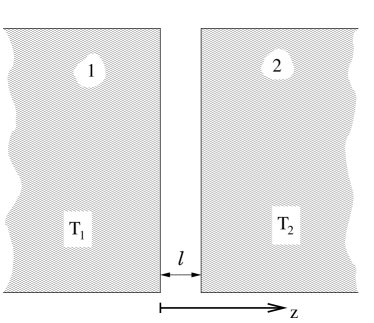
Figure 1: Schematic figure of the surface-surface system out of thermal equilibrium. Here the two bodies occupy infinite half-spaces.

The electromagnetic pressure between the two bodies along $z$ can be calculated as LLPCM ; Forcebetween

$$P^{\textrm{neq}}(T_{1},T_{2},l)=\langle T_{zz}({\bf r},t)\rangle,$$ (1)

that should be regularized by subtracting the same expression at separation $l\rightarrow\infty$. In Eq.(1), ${\bf r}$ is a generic point between the two bodies, and

$$T_{zz}({\bf r},t)=-\frac{\Lambda_{\alpha\beta}}{8\pi}\left[E_{\alpha}({\bf r},t)E_{\beta}({\bf r},t)+B_{\alpha}({\bf r},t)B_{\beta}({\bf r},t)\right],$$ (2)

is the $zz$ component of the Maxwell stress tensor in the vacuum gap. Here $\Lambda_{\alpha\beta}$ is a diagonal matrix with $\Lambda_{11}=\Lambda_{22}=1$ and $\Lambda_{33}=-1$.

To calculate the pressure (1) one must average over the state of the electromagnetic field the squares of the spatial components of the electric and magnetic field ${\bf E}({\bf r},t)$ and ${\bf B}({\bf r},t)$, which appear in Eq. (2).

Before starting with the analysis of the problem we mention the structure of this work in the following outline. In Sec. II we develop the formalism, introduce the role and the description of the fluctuations of the electromagnetic field and specify the approach we adopt to deal with the surface optics. In Sec. III we recall the main results of the surface-surface Casimir-Lifshitz interaction at thermal equilibrium, and in particular specify the distinction between the $T=0$ (purely quantum) and the thermal contribution to the force, generated by the radiation pressure of the thermal radiation. In Sec. IV we present a detailed derivation of the surface-surface pressure out of thermal equilibrium $P^{\textrm{neq}}(T_{1},T_{2},l)$. In Sec. V we show an alternative and useful expression for $P^{\textrm{neq}}(T_{1},T_{2},l)$, together with numerical results relative to particular couples of dielectric materials (i.e. fused silica-silicon and sapphire-fused silica). In Sec. VI we deal with the distance-independent terms in the pressure due to the finite thickness of the two bodies, and the eventual effect of external radiation at different temperature impinging the external surfaces. In Sec. VII we derive the large distance behavior of the surface-surface pressure out of thermal equilibrium, and discuss the role of the propagating waves (PW) and evanescent waves (EW) contributions. We also make a comparison with the corresponding terms of the pressure at thermal equilibrium. In Sec. VIII we consider the interaction between a surface and a rarefied body and derive the large distance behaviors of the PW and EW components. In the same section we stress the presence of non additivity in the interaction out of equilibrium (in contrast with the equilibrium case) and show the analysis of the crossing between different asymptotic behaviors. In Sec. IX we show the transition from the surface-rarefied body to surface-atom interactions out of thermal equilibrium, and demonstrate the essential role of finite thickness of the rarefied body. Finally in Sec. X we provide our conclusions.

In appendix A we give some details on the expression of the Green functions we used in our calculation, and in appendix B we discuss in detail the force acting between a surface and a rarefied body of finite thickness.

II The Formalism

Our approach is based on the theory of the fluctuating electromagnetic (EM) field developed by Rytov Rytov . In this approach it is assumed that the field is driven by randomly fluctuating current density or, alternatively, by randomly fluctuating polarization field. In this respect the Maxwell equations become of Langevin-type. For a monochromatic field in a non-homogeneous, linear, and nonmagnetic medium with the dielectric function $\varepsilon(\omega,\textbf{r})$ the Maxwell equations become:

$$\nabla\wedge{\bf E}[\omega;{\bf r}]-ik\;{\bf B}[\omega;{\bf r}] = 0,$$ (3)

$$\nabla\wedge{\bf B}[\omega;{\bf r}]+ik\;\varepsilon(\omega;{\bf r}){\bf E}[\omega;{\bf r}] = -4\pi\;ik\;{\bf P}[\omega;{\bf r}],$$ (4)

where $k=\omega/c$ is the vacuum wavenumber, and $\wedge$ is the vector product symbol. The source of the electromagnetic fluctuations is described by the electric polarization ${\bf P}[\omega;{\bf r}]$, related to the electric current density as ${\bf J}[\omega;{\bf r}]=-i\omega{\bf P}[\omega;{\bf r}]$. We use the following notations for the frequency Fourier transforms $A[\omega;{\bf r}]$ of the quantity $A(t,{\bf r})$:

$$A(t,{\bf r})=\int_{-\infty}^{+\infty}\frac{\textrm{d}\omega}{2\pi}e^{-i\omega t}A[\omega;{\bf r}].$$ (5)

To find the solution of the Maxwell equations we use the Green functions formalism. A Green function is a solution of the wave equation for a point source in presence of surrounding matter. When this solution is known one can construct the solution due to a general source using the principle of linear superposition. This method takes into account the effects of non-additivity, which originates from the fact that the interaction between two fluctuating dipoles is influenced by the presence of a third dipole. Employing this formalism we can express the electric field at the observation point ${\bf r}$ as the convolution

$${\bf E}\left[\omega;{\bf r}\right]=\int\overline{{\bf G}}\left[\omega;{\bf r},{\bf r}^{\prime}\right]\;\cdot{\bf P}\left[\omega;{\bf r}^{\prime}\right]\;\textrm{d}{\bf r}^{\prime}.$$ (6)

Here ${\bf P}\left[\omega;{\bf r}^{\prime}\right]$ is the random polarization at the source point ${\bf r}^{\prime}$, and $\overline{{\bf G}}\left[\omega;{\bf r},{\bf r}^{\prime}\right]$ is the dyadic Green function of the system. Then it is clear that the Green function plays the role of the response function in a linear-response theory. The Green function is the solution of the following equation LLP

$$\left\{\nabla\wedge\nabla\wedge-k^{2}\varepsilon(\omega,{\bf r})\right\}\overline{{\bf G}}[\omega;{\bf r},{\bf r}^{\prime}]=4\pi k^{2}\overline{{\bf I}}\delta({\bf r}-{\bf r}^{\prime}),$$ (7)

where $\overline{{\bf I}}$ is the identity dyad. This equation, resulting from the Maxwell equations (3) and (4) and convolution (6), has to be solved with proper boundary conditions characterizing the fields components at the interfaces, as well as the condition required by a retarded Green’s function retarded , i.e. $\overline{{\bf G}}[\omega;{\bf r},{\bf r}^{\prime}]\rightarrow 0$ as $|{\bf r}-{\bf r}^{\prime}|\rightarrow\infty$.

Finally it is useful to recall the relations $G_{\alpha\beta}[\omega;{\bf r},{\bf r}^{\prime}]=G_{\beta\alpha}[\omega;{\bf r}^{\prime},{\bf r}]$ and $G_{\alpha\beta}^{*}[\omega;{\bf r},{\bf r}^{\prime}]=G_{\alpha\beta}[-\omega;{\bf r},{\bf r}^{\prime}]$, that are the consequence of the microscopic reversibility in the linear-response theory and the reality of the time dependent fields, respectively.

II.1 Field correlation functions

From Eq.(1) it is evident that we are interested in the time correlations between different components of the electric (magnetic) field at equal times. In the quantum theory such correlations are described by the averages of symmetrized products of the field components:

$$\!\!\!\!\!\!\left\langle E_{\alpha}(\mathbf{r},t)E_{\beta}(\mathbf{r}^{\prime},t)\right\rangle_{\textrm{sym}}\equiv$$ (8)

$$\frac{1}{2}\left\langle E_{\alpha}(\mathbf{r},t)E_{\beta}(\mathbf{r}^{\prime},t)+E_{\beta}(\mathbf{r}^{\prime},t)E_{\alpha}(\mathbf{r},t)\right\rangle.$$

Notice that, although in this paper we are using symmetrized correlations, other possible forms of the correlation functions could be more appropriate in other situations Agarwal . The correlations (8) in terms of their Fourier transforms can be presented as

$$\!\!\!\!\!\!\left\langle E_{\alpha}(\textbf{r},t)E_{\beta}(\textbf{r}^{\prime},t)\right\rangle_{\textrm{sym}}=$$ (9)

$$\!\!\!\!\!\!\iint\frac{\textrm{d}\omega}{2\pi}\frac{\textrm{d}\omega^{\prime}}{2\pi}e^{-i(\omega-\omega^{\prime})t}\left\langle E_{\alpha}[\omega;\textbf{r}]\;E^{{\dagger}}_{\beta}[\omega^{\prime};\textbf{r}^{\prime}]\right\rangle_{\textrm{sym}}.$$

Using Eq.(6) these correlations can be expressed via the correlations of the polarization field $\bf P$, which obeys the fluctuation-dissipation theorem LLPCM

$$\!\!\!\!\!\!\left\langle P_{\alpha}[\omega;{\textbf{r}}]P_{\beta}^{{\dagger}}[\omega^{\prime};{\textbf{r}}^{\prime}]\right\rangle_{\textrm{sym}}=$$ (10)

$$\!\!\!\!\!\!\frac{\hbar\varepsilon^{\prime\prime}(\omega,\textbf{r})}{2}\coth\left(\frac{\hbar\omega}{2k_{B}T}\right)\delta(\omega-\omega^{\prime})\delta({\bf r}-{\bf r}^{\prime})\delta_{\alpha\beta},$$

expressed via the Fourier transformed ${\bf P}\left[\omega;\textbf{r}\right]$. Due to the presence of the $\delta\left({\bf r}-{\bf r}^{\prime}\right)$ factor these fluctuations are local. Fluctuations of the sources in different points of the material are non-coherent. This permits to assume that in the non-equilibrium situation, when temperature $T$ is different in different points, the sources correlations are given by the same equations. We must emphasize that this assumption, even being quite reasonable, is still a hypothesis, which is worth both of further theoretical investigation and experimental verification. The problem was discussed previously (see particularly Eckhardt ), but in our opinion the conditions of applicability of the theory has not been still established. The same assumption was used by Polder and Van Hove Polder to calculate the radiative heat transfer between two bodies with different temperatures.

The assumption (10) (local source hypothesis) represents the starting point of our analysis allowing for an explicit calculation of the electromagnetic field also if the system is not in global thermal equilibrium.

It is now evident that EM field in the vacuum gap is given by the sum of the fields produced by the fluctuating polarizations in the materials filling respectively the half-space $1$, with the dielectric function $\varepsilon_{1}(\omega)$ and temperature $T_{1}$, and the half-space $2$ with the dielectric function $\varepsilon_{2}(\omega)$ and temperature $T_{2}$. Then the Fourier transform of the electric field correlations can be presented as

$$\left\langle E_{\alpha}[\omega;\textbf{r}]E_{\beta}^{{\dagger}}[\omega^{\prime};\textbf{r}^{\prime}]\right\rangle_{\textrm{sym}}=\left[\frac{\hbar\varepsilon^{\prime\prime}_{1}(\omega)}{2}\coth\left(\frac{\hbar\omega}{2k_{B}T_{1}}\right)S_{\alpha\beta}^{(1)}\left[\omega;{\bf r},{\bf r}^{\prime}\right]+\frac{\hbar\varepsilon^{\prime\prime}_{2}(\omega)}{2}\coth\left(\frac{\hbar\omega}{2k_{B}T_{2}}\right)S_{\alpha\beta}^{(2)}\left[\omega;{\bf r},{\bf r}^{\prime}\right]\right]\delta\left(\omega-\omega^{\prime}\right),$$ (11)

where $S^{(i)}_{\alpha\beta}\ (i=1,2)$ is defined as convolution of two Green functions

$$S^{(i)}_{\alpha\beta}\left[\omega;{\bf r},{\bf r}^{\prime}\right]=\int_{V_{i}}d{\bf r}^{\prime\prime}G_{\alpha\gamma}[\omega;{\bf r},{\bf r}^{\prime\prime}]G_{\gamma\beta}^{*}[\omega;{\bf r}^{\prime\prime},{\bf r}^{\prime}].$$ (12)

Here $V_{1}$ and $V_{2}$ are the volumes occupied by the left and right body, respectively, and the two terms in Eq.(11) correspond to the parts of the pressure generated by the sources in each body separately.

It is interesting to see how the global equilibrium is restored when $T_{1}\rightarrow T_{2}=T$ in Eq. (11). In this case Eq. (11) can be written as

$$\!\!\!\!\!\!\!\left\langle E_{\alpha}[\omega;\textbf{r}]E_{\beta}^{{\dagger}}[\omega^{\prime};\textbf{r}^{\prime}]\right\rangle_{\textrm{sym}}=\frac{\hbar}{2}\coth\left(\frac{\hbar\omega}{2k_{B}T}\right)\delta\left(\omega-\omega^{\prime}\right)\times$$ (13)

$$\!\!\!\!\int_{V_{1}+V_{2}}d{\bf r}^{\prime\prime}\varepsilon^{\prime\prime}(\omega,{\bf r}^{\prime\prime})G_{\alpha\gamma}[\omega;{\bf r},{\bf r}^{\prime\prime}]G_{\gamma\beta}^{*}[\omega;{\bf r}^{\prime\prime},{\bf r}^{\prime}].$$

The integral over the product of two Green functions is connected with the imaginary part of the single Green function by the important Eckhardt ; Kazarinov relation

$$\!\!\!\!\!\!\!\!\!\!\!\!\!\!\!\int_{\Omega}d{\bf r}^{\prime\prime}\varepsilon^{\prime\prime}(\omega,{\bf r}^{\prime\prime})G_{\alpha\gamma}[\omega;{\bf r},{\bf r}^{\prime\prime}]G_{\gamma\beta}^{*}[\omega;{\bf r}^{\prime\prime},{\bf r}^{\prime}]=$$ (14)

$$\;\;\;\;\;\;\;\;\;\;\;\;\;\;\;\;\;\;\;\;\;\;\;\;\;\;\;\;\;\;\;\;\;4\pi\textrm{Im}G_{\alpha\beta}[\omega;{\bf r},{\bf r}^{\prime}],$$

where $\Omega$ is a volume restricted by a surface where the Green function vanishes. Keeping in mind that in the vacuum gap $\varepsilon^{\prime\prime}=0$, one can extend the integration in Eq. (13) over the the whole space and using (14) one recovers the well-known form of the electric fields fluctuation-dissipation theorem LLP valid at a global thermal equilibrium:

$$\!\!\!\!\!\left\langle E_{\alpha}[\omega;\textbf{r}]E_{\beta}^{{\dagger}}[\omega^{\prime};\textbf{r}^{\prime}]\right\rangle_{\textrm{sym}}=$$ (15)

$$2\pi\hbar\coth\left(\frac{\hbar\omega}{2k_{B}T}\right)\textrm{Im}G_{\alpha\beta}[\omega;{\bf r},{\bf r}^{\prime}]\delta\left(\omega-\omega^{\prime}\right).$$

Notice that all fluctuations presented in this section include both the vacuum ($T=0$) and the thermal fluctuations. These can be identified with the first and second terms, respectively, of the r.h.s. of the identity

$$\coth\left(\frac{\hbar\omega}{2k_{B}T}\right)=\textrm{sign}(\omega)\left(1+\frac{2}{e^{\hbar|\omega|/k_{B}T}-1}\right),\;\;\;\omega\neq 0.$$ (16)

II.2 The pressure in terms of fluctuations

The pressure (1) can be presented in terms of the Fourier transformed fields correlations:

$$\!\!\!\!\!\!\!\!\!\!\!\!\!\!\!\!P^{\textrm{neq}}(T_{1},T_{2},l)=-\frac{1}{8\pi}\iint\frac{\textrm{d}\omega}{2\pi}\frac{\textrm{d}\omega^{\prime}}{2\pi}e^{-i(\omega-\omega^{\prime})t}\;\times$$ (17)

$$\;\;\;\;\;\;\;\;\Lambda_{\alpha\beta}\left[\left\langle E_{\alpha}[\omega;{\bf r}]E^{{\dagger}}_{\beta}[\omega^{\prime};{\bf r}^{\prime}]\right\rangle+\right.$$

$$\left.\;\;\;\;\;\;\;\;\;\;\;\;\;\;\;\;\;\;\;\;\left\langle B_{\alpha}[\omega;{\bf r}]B^{{\dagger}}_{\beta}[\omega^{\prime};{\bf r}^{\prime}]\right\rangle\right]\Big{|}_{{\bf r}={\bf r}^{\prime}}.$$

Here the electric and magnetic contributions to the total pressure are explicit, and ${\bf r}$ is a point inside of the vacuum gap. The stress tensor is in fact constant in the vacuum gap due to the momentum conservation required by a stationary configuration (see discussion in section IV.1). In this equation we omitted the symmetrization index since the average is taken at the same point ${\bf r}={\bf r}^{\prime}$. Using Eq.(3) it is useful to rewrite expression (17) in terms of the electric fields only Matloob as

$$\!\!\!\!\!\!\!P^{\textrm{neq}}(T_{1},T_{2},l)=-\frac{1}{8\pi}\iint\frac{\textrm{d}\omega}{2\pi}\frac{\textrm{d}\omega^{\prime}}{2\pi}e^{-i(\omega-\omega^{\prime})t}\times$$ (18)

$$\;\;\;\;\;\;\;\;\;\;\;\;\;\;\;\;\;\;\;\;\Theta_{\delta\nu}\left[\left\langle E_{\delta}[\omega;{\bf r}]E^{{\dagger}}_{\nu}[\omega^{\prime};{\bf r}^{\prime}]\right\rangle\right]\Big{|}_{{\bf r}={\bf r}^{\prime}}.$$

Here the pressure is expressed in terms of the correlations (11), and the operator

$$\Theta_{\delta\nu}=\Lambda_{\alpha\beta}\left(\delta_{\alpha\delta}\delta_{\beta\nu}+\frac{1}{k^{2}}\epsilon_{\alpha\gamma\delta}\epsilon_{\beta\eta\nu}\partial_{\gamma}\partial^{\prime}_{\eta}\right)$$ (19)

selects the electric and magnetic contributions, given by the first and the second term in Eq.(19), respectively.

From Eq.(16) it is possible to express the total pressure as the sum

$$P^{\textrm{neq}}(T_{1},T_{2},l)=P_{0}(l)+P_{\textrm{th}}^{\textrm{neq}}(T_{1},T_{2},l),$$ (20)

where the contribution of the zero-point ($T=0$) fluctuations, $P_{0}(l)$, is separated from that produced by the thermal fluctuations, $P_{\textrm{th}}^{\textrm{neq}}(T_{1},T_{2},l)$. Furthermore, thanks to equation (11) it is possible to express the thermal component of the pressure acting between the bodies as the sum of two terms

$$P_{\textrm{th}}^{\textrm{neq}}(T_{1},T_{2},l)=P_{\textrm{th}}^{\textrm{neq}}(T_{1},0,l)+P_{\textrm{th}}^{\textrm{neq}}(0,T_{2},l).$$ (21)

The pressure at thermal equilibrium $P^{\textrm{eq}}(T,l)$, being a particular case of (20), can be written as

$$P^{\textrm{eq}}(T,l)=P_{0}(l)+P_{\textrm{th}}^{\textrm{eq}}(T,l).$$ (22)

The pressures $P_{0}(l)$ and $P_{\textrm{th}}^{\textrm{eq}}(T,l)$ are given by Eq.(18), where the field fluctuations are provided by Eq. (15) after the substitution, respectively, of:

$$\coth\left(\frac{\hbar\omega}{2k_{B}T}\right)\rightarrow\textrm{sign}(\omega),$$ (23)

$$\coth\left(\frac{\hbar\omega}{2k_{B}T}\right)\rightarrow\frac{2\;\textrm{sign}(\omega)}{e^{\hbar|\omega|/k_{B}T}-1}.$$ (24)

If one simply perform such substitutions, it is well know that equation (18) diverges at $T=0$, and contains constant ($l$-independent) terms in the thermal part. The divergence has the same origin as the usual divergence of the zero-point fields energy in quantum electrodynamics, while the constant terms are related to the fact that we consider infinite bodies, and hence we neglect the pressure of the radiation exerted on the remote, external surfaces of the two bodies. To recover the exact finite value for the pressures $P_{0}(l)$, and exclude the constant terms in $P_{\textrm{th}}^{\textrm{eq}}(T,l)$, one should regularize the Green function in the r.h.s of Eq.(15) by subtracting the bulk part $G_{ij}^{\textrm{bu.}}$, corresponding to a field produced by a point-like dipole in an homogeneous and infinite dielectric LP ; TomasLif ; Tomas95 . In fact, the Green function with both the observation point ${\bf r}$ and the source point ${\bf r}^{\prime}$ in the vacuum gap (see section A.1) is given by the sum

$$G_{ij}\left[\omega;{\bf r},{\bf r}^{\prime}\right]=G_{ij}^{\textrm{sc.}}\left[\omega;{\bf r},{\bf r}^{\prime}\right]+G_{ij}^{\textrm{bu.}}\left[\omega;{\bf r},{\bf r}^{\prime}\right],$$ (25)

of a scattered and a bulk term. The subtraction of the bulk term corresponds to the subtraction of the pressure at $l\rightarrow\infty$, as prescribed after Eq.(1). The expressions for the pressure at thermal equilibrium are given explicitly in section III.

Concerning the thermal pressure out of thermal equilibrium $P_{\textrm{th}}^{\textrm{neq}}(T_{1},T_{2},l)$ of Eq. (20), it can be obtained from Eq.(18) by using (11) and the substitution (24). Also in this case the thermal pressure $P_{\textrm{th}}^{\textrm{neq}}(T_{1},T_{2},l)$ contains an $l$-dependent and a constant term, as it happens for $P_{\textrm{th}}^{\textrm{eq}}(T,l)$ before being regularized. Differently from the equilibrium case, here the origin of the constant terms is not only due to the absence of the pressure acting on the remote surfaces, but is also related to the fact that out of thermal equilibrium there is a net momentum transfer between the bodies. In this case the constant terms can remain also after considering bodies of finite thickness, and can even be different for the two bodies, depending on the external radiations. In the sections IV and V we will calculate $P_{\textrm{th}}^{\textrm{neq}}(T_{1},T_{2},l)$ for two bodies filling two infinite half-spaces, and we will mainly discuss the pure $l$-dependent component. The constant terms will be discussed in section VI for the general case of bodies of finite thickness, with impinging the external radiations at different temperatures.

II.3 Electromagnetic waves in surface optics

In this work we formulate the electromagnetic problem in terms of $s$- and $p$-polarized vector waves and in terms of the Fresnel coefficients for the interfaces Sipe . Such notations are very useful in surface optics. We will also employ the angular spectrum representation for the description of the EM and polarization vectors.

If $\hat{\bf{x}},\hat{\bf{y}}$ and $\hat{\bf{z}}$ are the coordinate unit vectors (with real norm equal to $1$), one can write the position vector as ${\bf r}={\bf R}+z\;\hat{\bf{z}}$, where the capital letter refers to vectors parallel to the interface [${\bf R}\equiv(R_{x},R_{y},0)$]. Let us write the electromagnetic (complex) wave vector in the medium $m$ with the complex dielectric function $\varepsilon_{m}(\omega)=\varepsilon_{m}^{\prime}(\omega)+i\varepsilon_{m}^{\prime\prime}(\omega)$ as

$${\bf q}^{(m)}(\pm)={\bf Q}\pm q_{z}^{(m)}\;\hat{\bf z}.$$ (26)

Here the sign $(+)$ corresponds to an upward-propagating (or evanescent) wave, and the sign $(-)$ corresponds to a downward-propagating (or evanescent) wave. The vector ${\bf Q}\equiv(Q_{x},Q_{y},0)$ is the projection (always real) of ${\bf q}^{(m)}(\pm)$ on the interface and the $z-$component of the wave vector, and

$$q_{z}^{(m)}=\sqrt{\varepsilon_{m}\;k^{2}-Q^{2}},$$ (27)

is a complex number with a positive imaginary part, and positive real part in case $\textrm{Im}q_{z}^{(m)}=0$. Real and imaginary parts of $q_{z}^{(m)}$ are expressed by the following relations:

$$\textrm{Re}q_{z}^{(m)}=\sqrt{\frac{1}{2}\left[|\varepsilon_{m}(\omega)k^{2}-Q^{2}|+(\varepsilon_{m}^{\prime}(\omega)k^{2}-Q^{2})\right]},$$ (28)

$$\textrm{Im}q_{z}^{(m)}=\sqrt{\frac{1}{2}\left[|\varepsilon_{m}(\omega)k^{2}-Q^{2}|-(\varepsilon_{m}^{\prime}(\omega)k^{2}-Q^{2})\right]}.$$ (29)

Then, if the medium $m$ is non-absorbing ($\varepsilon_{m}^{\prime\prime}=0$), for $Q\leq\sqrt{\varepsilon_{m}^{\prime}}\;k$ the wavevector $q_{z}^{(m)}$ is real and corresponds to a wave propagating in the medium $m$, while for $Q>\sqrt{\varepsilon_{m}^{\prime}}\;k$ the wavevector $q_{z}^{(m)}$ is imaginary and corresponds to evanescent wave in the medium $m$. The following identities will be useful:

$$2\;\textrm{Im}\;q_{z}^{(m)}\;\textrm{Re}\;q_{z}^{(m)} = k^{2}\;\varepsilon_{m}^{\prime\prime}(\omega),$$ (30)

$$\left(Q^{2}+|q_{z}^{(m)}|^{2}\right)\textrm{Re}\;q_{z}^{(m)} = k^{2}\;\textrm{Re}\left(\varepsilon_{m}^{*}(\omega)\;q_{z}^{(m)}\right),$$ (31)

$$\left(Q^{2}-|q_{z}^{(m)}|^{2}\right)\textrm{Im}\;q_{z}^{(m)} = k^{2}\;\textrm{Im}\left(\varepsilon_{m}^{*}(\omega)\;q_{z}^{(m)}\right).$$ (32)

It is worth noticing that the wave vectors ${\bf q}^{(m)}(\pm)$ lie in the plane of incidence spanned by $\hat{\bf Q}$ and $\hat{\bf z}$. Than one can introduce the $s$- and $p$-unit complex polarization vectors

$${\bf e}_{s}^{(m)}(\pm)=\hat{\bf Q}\wedge\hat{\bf z},$$ (33)

$${\bf e}_{p}^{(m)}(\pm)={\bf e}_{s}^{(m)}(\pm)\wedge\hat{\bf q}^{(m)}(\pm)=\frac{Q\hat{\bf z}\mp q_{z}^{(m)}\hat{\bf Q}}{\sqrt{\varepsilon_{m}(\omega)}\;k},$$ (34)

that are vectors transversal and longitudinal to that plane, respectively. Usually the polarization vector ${\bf e}_{s}^{(m)}(\pm)$ [${\bf e}_{p}^{(m)}(\pm)$] is called transverse electric (TE) [transverse magnetic (TM)] since it corresponds to the electric [magnetic] field transverse to the plane of incidence.

Our geometry consists of two half-spaces labeled with $m=1,2$ separated by a vacuum gap. Inside of the gap the wave vector ${\bf q}$ and the polarization vectors ${\bf e}_{\mu}(\pm)$ are not labeled and are obtained, respectively, from the definitions (26), (27) and (33), (34) by omitting the apices ^(m), and setting $\varepsilon_{m}=1$.

Finally we can introduce the well known reflection and transmission Fresnel coefficients for the vacuum gap-dielectric interfaces, which for the $s$- and $p$-wave components are:

$$r^{s}_{m}=\frac{q_{z}-q_{z}^{(m)}}{q_{z}+q_{z}^{(m)}} r^{p}_{m}=\frac{q_{z}\varepsilon_{m}-q_{z}^{(m)}}{q_{z}\varepsilon_{m}+q_{z}^{(m)}},$$ , (35)

$$t^{s}_{m}=\frac{2\,q_{z}^{(m)}}{q_{z}^{(m)}+q_{z}} t^{p}_{m}=\frac{2\;\sqrt{\varepsilon_{m}(\omega)}\;q_{z}^{(m)}}{q_{z}^{(m)}+q_{z}\varepsilon_{m}(\omega)}.$$ , (36)

In particular, the coefficients $r_{m}$ relate the radiation in the vacuum gap impinging the interface $m$ and its part reflected back into the vacuum gap. The coefficients $t_{m}$ relate the radiation impinging the interface $m$ from the interior of the dielectric $m$ and its part transmitted into the vacuum gap (see Appendix A).

III Pressure at thermal equilibrium

In this section we briefly recall the main results of the pressure in a system at thermal equilibrium. We present the thermal component of the pressure as the sum of PW and EW components, and in terms of real frequencies, which will result useful for the rest of the discussion. The results we show for the pressure at equilibrium are regularized [see discussion after Eq.(24)].

The Lifshitz surface-surface pressure at thermal equilibrium can be expressed in terms of real frequencies as

$$P^{\textrm{eq}}(T,l) = -\frac{\hbar}{2\pi^{2}}\int_{0}^{\infty}\textrm{d}\omega\coth{\left(\frac{\hbar\omega}{2k_{B}T}\right)}$$ (37)

$$\times\textrm{Re}\left[\int_{0}^{\infty}\textrm{d}Q\;Q\;q_{z}\;g(Q,\omega)\right],$$

where

$$g(Q,\omega) = \sum_{\mu=s,p}\frac{r^{\mu}_{1}r^{\mu}_{2}e^{2iq_{z}l}}{D_{\mu}}$$ (38)

$$= \sum_{\mu=s,p}\left[(r^{\mu}_{1}r^{\mu}_{2})^{-1}e^{-2iq_{z}l}-1\right]^{-1}.$$

In the previous equation the multiple reflections are described by the factor

$$D_{\mu}=1-r^{\mu}_{1}r^{\mu}_{2}e^{2iq_{z}l},$$ (39)

and the reflection Fresnel coefficients $r^{\mu}_{m}$ for the vacuum-dielectric interfaces are defined in Eq.(35).

By performing the Lifshitz rotation on the complex plane it is possible to write Eq.(37) in terms of imaginary frequencies:

$$P^{\textrm{eq}}(T,l) = \frac{k_{B}\;T}{16\pi l^{3}}\int_{0}^{\infty}\textrm{d}x\;x^{2}\bigg{[}\frac{(\varepsilon_{10}+1)(\varepsilon_{20}+1)}{(\varepsilon_{10}-1)(\varepsilon_{20}-1)}e^{x}-1\bigg{]}^{-1}$$ (40)

$$+ \frac{k_{B}T}{\pi c^{3}}\sum_{n=1}^{\infty}\xi^{3}_{n}\int_{1}^{\infty}\textrm{d}p\;p^{2}\;g(p,i\xi_{n}),$$

where $p=\sqrt{1+c^{2}Q^{2}/\xi_{n}^{2}}$. The dielectric functions that enter to $g(p,i\xi_{n})$ must be evaluated at imaginary frequencies $\varepsilon_{1,2}=\varepsilon_{1,2}(i\xi_{n})$, where $\xi_{n}=2\pi k_{B}Tn/\hbar$. In the first term of (40) we have also introduced the static values of the dielectric functions $\varepsilon_{10}=\varepsilon_{1}(0)$ and $\varepsilon_{20}=\varepsilon_{2}(0)$.

The pressure at thermal equilibrium includes contributions from zero-point fluctuations $P_{0}(l)$ and from thermal fluctuations $P_{\textrm{th}}^{\textrm{eq}}(T,l)$ as Eq. (22) shows. $P_{0}(l)$ can be extracted from (37) with the substitutes (23) or from (40) as the limit of continuous imaginary frequency. The final result for the $T=0$ pressure is

$$P_{0}(l)=\frac{\hbar}{2\pi^{2}c^{3}}\int_{0}^{\infty}\textrm{d}\xi\int_{1}^{\infty}\textrm{d}p\;p^{2}\xi^{3}\;g(p,i\xi).$$ (41)

The pressure $P_{0}(l)$ admits two important limits, i.e. the Van der Waals-London and the Casimir-Polder behaviors, valid at small and large distances, respectively, in respect to the characteristic length scale $\lambda_{opt}$ fixed by the absorption spectrum of the bodies (typically is of the order of fraction of microns).

The behavior of the thermal component $P_{\textrm{th}}^{\textrm{eq}}(T,l)$ is related to a second length scale, i.e. the thermal wavelength

$$\lambda_{T}\equiv\frac{\hbar c}{k_{B}T},$$ (42)

which at room temperature is $\approx 7.6\;\mu m$.

Then, the zero-point fluctuations dominate over the thermal contribution at small distances $l\ll\lambda_{T}$. In this limit behavior of the pressure is determined by the characteristic length scale $\lambda_{opt}\ll\lambda_{T}$. In the interval $\lambda_{opt}\ll l\ll\lambda_{T}$ one enters the Casimir-Polder regime where the pressure decays like $1/l^{4}$. For distances $l\ll\lambda_{opt}$ the force instead exhibits the $1/l^{3}$ van der Waals-London dependence. The possibility of identifying the Casimir-Polder regime depends crucially on the value of the temperature. The temperature should be in fact sufficiently low in order to guarantee the condition $\lambda_{T}\gg\lambda_{opt}$.

The last part of this section focuses on the thermal component of the pressure, that will be often used along the rest of the paper. The pressure $P_{\textrm{th}}^{\textrm{eq}}(T,l)$ can be obtained from (37) by using (24). Since such a component of the pressure will be compared with that out of thermal equilibrium, we show here explicitly its expression for PW and EW contributions:

$$P_{\textrm{th}}^{\textrm{eq,PW}}(T,l) = -\frac{\hbar}{\pi^{2}}\int_{0}^{\infty}\textrm{d}\omega\frac{1}{e^{\hbar\omega/k_{B}T}-1}\int_{0}^{k}\textrm{d}Q\;Q\;q_{z}\;\sum_{\mu=s,p}\frac{\textrm{Re}\left(r^{\mu}_{1}r^{\mu}_{2}\;e^{2iq_{z}l}\right)-|r^{\mu}_{1}\;r^{\mu}_{2}|^{2}}{|D_{\mu}|^{2}},$$ (43)

$$P_{\textrm{th}}^{\textrm{eq,EW}}(T,l) = \frac{\hbar}{\pi^{2}}\int_{0}^{\infty}\textrm{d}\omega\frac{1}{e^{\hbar\omega/k_{B}T}-1}\int_{k}^{\infty}\textrm{d}Q\;Q\;\textrm{Im}q_{z}\;e^{-2l\textrm{Im}q_{z}}\;\sum_{\mu=s,p}\frac{\textrm{Im}\left(r^{\mu}_{1}r^{\mu}_{2}\right)}{|D_{\mu}|^{2}}.$$ (44)

In particular at high temperatures, or equivalently at large distances defined by the condition

$$l\gg\lambda_{T},$$ (45)

the leading contribution to the pressure is given by the expression for the total force LP

$$P_{\text{th}}^{\text{eq}}(T,l)=\frac{k_{B}T}{16\pi l^{3}}\int_{0}^{\infty}\!\!\!\textrm{d}x\;x^{2}\;\left[\frac{\varepsilon_{10}+1}{\varepsilon_{10}-1}\frac{\varepsilon_{20}+1}{\varepsilon_{20}-1}\;e^{x}-1\right]^{-1}.$$ (46)

It corresponds to the first term in Eq.(40) and is entirely due to the thermal fluctuations of the EM field. In Ref. LP the asymptotic behavior (46) has been found after the contour rotation in the complex $\omega$-plane of the EW term (44), that is partially canceled by the PW term (43).

One can note that in this regime only the static value of the dielectric functions is relevant. The pressure (46) is proportional to the temperature, is independent from the Planck constant as well as from the velocity of light. We will call this equation the Lifshitz limit. The pressure (46) can be obtained from the thermal free energy $\mathcal{F}=\mathcal{E}-T\mathcal{S}$ of the electromagnetic field (per unit area) according to the thermodynamic identity $P=-\left(\partial\mathcal{F}/\partial l\right)_{T}$, where $\mathcal{E}$ and $\mathcal{S}$ are the thermal energy and entropy, respectively. It is interesting to note that, differently from the free energy, the thermal energy $\mathcal{E}$ decreases exponentially with $l$, which means that the pressure (46) has pure entropic origin Revzen .

It is important that at large separations only the $p$-polarization contributes to the force (see for, example in AntezzaPhDthesis , the detailed derivation of the PW and EW components). The reason is that for low-frequencies the $s$-polarized field is nearly pure magnetic, but the magnetic field penetrates freely into a non-magnetic material Sve05 .

In the limit $\varepsilon_{10},\varepsilon_{20}\rightarrow\infty$ we find the force between two metals

$$P_{\text{th}}^{\text{eq,met}}(T,l)=\frac{k_{B}T}{8\pi l^{3}}\;\zeta(3).$$ (47)

Let us empathize that this result was obtained for interaction between real metals Bos00 . For ”ideal mirrors” considered by Casimir, both polarizations of electromagnetic fields are reflected. In this case there will be an additional factor 2 in Eq.(46) due to the contribution of the $s-$polarization. This ideal case can be realized using superconducting mirrors.

It is useful to note that the surface-surface pressure $P^{\textrm{eq}}(T,l)$ given by the Lifshitz result (40) hides a non trivial cancellation between the components of the pressure related to real and imaginary values of the EM wavevectors, leading, respectively, to the propagating (PW) and evanescent (EW) wave contributions articolo2 ; Intravaia . This study deserves careful investigation since for a configuration out of thermal equilibrium such cancellations are no longer present, and the PW and EW contribution will provide different asymptotic behaviors. The new effect, as we will see, is particularly important if one of the two bodies is a rarefied gas.

IV Pressure out of thermal equilibrium between two infinite dielectric half-spaces

As was discussed above [see Eqs. (11) and (21)] each body contributes separately to the thermal pressure. In particular the pressure resulting from the thermal fluctuations in the body $1$ is

$$\;\;P_{\textrm{th}}^{\textrm{neq}}(T,0,l)=$$

$$\!\!\!\!\!\!-\frac{\hbar}{16\pi^{3}}\int_{0}^{\infty}\textrm{d}\omega\frac{\varepsilon_{1}^{\prime\prime}(\omega)}{e^{\hbar\omega/k_{B}T}-1}\textrm{Re}\left[\Theta_{\delta\nu}S_{\delta\nu}^{(1)}\left[\omega;{\bf r}_{1},{\bf r}_{2}\right]\right]\Big{|}_{{\bf r}_{1}={\bf r}_{2}},$$

where ${\bf r}_{1}={\bf r}_{2}$ is a point in the vacuum gap and the function $S$ is defined in Eq.(12). In Eq.(LABEL:LifForcesssLLss) we used the parity properties $\varepsilon^{\prime\prime}(\omega)=-\varepsilon^{\prime\prime}(-\omega)$ and $S_{\delta\nu}\left[\omega;{\bf r}_{1},{\bf r}_{2}\right]=S_{\delta\nu}^{*}\left[-\omega;{\bf r}_{1},{\bf r}_{2}\right]$ to restrict the range of integration to the positive frequencies. It is evident that $P_{\textrm{th}}^{\textrm{neq}}(0,T,l)$ can be expressed similarly to Eq.(LABEL:LifForcesssLLss), but with $\varepsilon_{1}^{\prime\prime}(\omega)\rightarrow\varepsilon_{2}^{\prime\prime}(\omega)$ and $S_{\delta\nu}^{(1)}\rightarrow S_{\delta\nu}^{(2)}$.

Below we specify the expressions of the tensors $S_{\delta\nu}^{(1)}$ and $S_{\delta\nu}^{(2)}$ (section IV.1), calculate the electric and magnetic contributions to the pressure (section IV.2), and finally provide the result for the total pressure in terms of PW and EW components (section IV.3). The total pressure will be rewritten in a different form in section V by using a powerful expansion in multiple reflections. In the present and in the next section V the pressure is calculated for two infinite bodies [see discussion at the end of section II.2].

IV.1 The $S$ functions

In this subsection we show the result for the tensors $S_{\delta\nu}^{(1)}$ and $S_{\delta\nu}^{(2)}$ defined by Eq. (12). In terms of the lateral Fourier transforms $s_{\delta\nu}^{(1)}[\omega;{\bf Q},z_{1},z_{2}]$ and $s_{\delta\nu}^{(2)}[\omega;{\bf Q},z_{1},z_{2}]$ one has

$$S_{\delta\nu}[\omega;{\bf r}_{1},{\bf r}_{2}]=\int\frac{\textrm{d}^{2}{\bf Q}}{(2\pi)^{2}}\;e^{i{\bf Q}\cdot\left({\bf R}_{1}-{\bf R}_{2}\right)}\;s_{\delta\nu}[\omega;{\bf Q},z_{1},z_{2}].$$ (49)

By choosing the $x$-axis parallel to the vector ${\bf D}={\bf R}_{1}-{\bf R}_{2}$ and defining $\phi$ as the angle between ${\bf Q}$ and ${\bf D}$ one gets that $Q_{x}=Q\cos\phi$, $Q_{y}=Q\sin\phi$ and the polarization vectors become

$$\!\!\!\!\!{\bf e}_{s}^{(m)}(\pm) = \left(|\sin\phi|,-\cos\phi\;\sin\phi/|\sin\phi|,0\right),$$ (50)

$$\!\!\!\!\!{\bf e}_{p}^{(m)}(\pm) = \frac{1}{\sqrt{\varepsilon_{m}}k}\left(\mp q_{z}^{(m)}\cos\phi,\mp q_{z}^{(m)}\sin\phi,Q\right).$$ (51)

Here it is evident that $|{\bf e}_{s}^{(m)}(\pm)|^{2}=1$ and

$$|{\bf e}_{p}^{(m)}(\pm)|^{2}=\frac{Q^{2}+|q_{z}^{(m)}|^{2}}{|\varepsilon_{m}|\;k^{2}}.$$ (52)

After explicit calculation using the Green function given in appendix A we find for the $s_{\delta\nu}^{(1)}$ and $s_{\delta\nu}^{(2)}$ functions the explicit expressions

$$s_{\delta\nu}^{(1)}[\omega;{\bf Q},z_{1},z_{2}] = \frac{4\pi^{2}k^{2}}{\varepsilon_{1}^{\prime\prime}(\omega)}\frac{\textrm{Re}q_{z}^{(1)}}{|q_{z}^{(1)}|^{2}}\;\sum_{\mu=s,p}\;\frac{|t_{1}^{\mu}|^{2}}{|D_{\mu}|^{2}}\;\;|{\bf e}_{\mu}^{(1)}(+)|^{2}\;\times$$ (53)

$$\left[e_{\mu,\delta}(+)e_{\mu,\nu}^{*}(+)\;e^{i(q_{z}z_{1}-q_{z}^{*}z_{2})}+e_{\mu,\delta}(+)e_{\mu,\nu}^{*}(-)\;e^{i(q_{z}z_{1}+q_{z}^{*}z_{2})}\;e^{-2iq_{z}^{*}l}\;r_{2}^{\mu*}+\right.$$

$$\left.e_{\mu,\delta}(-)e_{\mu,\nu}^{*}(+)\;e^{-i(q_{z}z_{1}+q_{z}^{*}z_{2})}\;e^{2iq_{z}l}\;r_{2}^{\mu}+e_{\mu,\delta}(-)e_{\mu,\nu}^{*}(-)\;e^{-i(q_{z}z_{1}-q_{z}^{*}z_{2})}\;e^{-4\textrm{Im}q_{z}l}\;|r_{2}^{\mu}|^{2}\right],$$

$$s_{\delta\nu}^{(2)}[\omega;{\bf Q},z_{1},z_{2}] = \frac{4\pi^{2}k^{2}}{\varepsilon_{2}^{\prime\prime}(\omega)}\;\frac{\textrm{Re}q_{z}^{(2)}}{|q_{z}^{(2)}|^{2}}\;e^{-2l\textrm{Im}q_{z}}\;\sum_{\mu=s,p}\;\frac{|t_{2}^{\mu}|^{2}}{|D_{\mu}|^{2}}\;\;|{\bf e}_{\mu}^{(2)}(-)|^{2}\;\times$$ (54)

$$\left[e_{\mu,\delta}(-)e_{\mu,\nu}^{*}(-)\;e^{-i(q_{z}z_{1}-q_{z}^{*}z_{2})}+e_{\mu,\delta}(-)e_{\mu,\nu}^{*}(+)\;e^{-i(q_{z}z_{1}+q_{z}^{*}z_{2})}\;r_{1}^{\mu*}+\right.$$

$$\left.e_{\mu,\delta}(+)e_{\mu,\nu}^{*}(-)\;e^{i(q_{z}z_{1}+q_{z}^{*}z_{2})}\;r_{1}^{\mu}+e_{\mu,\delta}(+)e_{\mu,\nu}^{*}(+)\;e^{i(q_{z}z_{1}-q_{z}^{*}z_{2})}\;|r_{1}^{\mu}|^{2}\right],$$

where $D_{\mu}$ is defined in Eq.(39).

It is worth noticing that in the non equilibrium but stationary regime the fields correlation functions $s^{(1,2)}$ are not uniform in the vacuum cavity, while on the contrary the Maxwell stress tensor $T_{zz}$ (which is related to the momentum flux) has the same value in each point of the vacuum gap. This is valid also at equilibrium, and is a direct consequence of the momentum conservation required by a stationary configuration. To show this property one can set $z_{1}=z_{2}=z$ in Eq.(53), where the dependence on $z$ appears only in the exponential factors [the same would happen for Eq.(54)] . Let us note that now the first and the last terms in such an expression are proportional to $e^{2z\textrm{Im}q_{z}}$ and $e^{-2z\textrm{Im}q_{z}}$, respectively, while the second and the third terms are proportional to $e^{-2z\textrm{Re}q_{z}}$ and $e^{2z\textrm{Re}q_{z}}$, respectively. As it will be clear in the next section IV.2 the first and the last terms will be responsible for the PW contribution to the pressure (for which $\textrm{Im}q_{z}=0$), while the second and the third terms will be responsible for the EW contribution (for which $\textrm{Re}q_{z}=0$). It is then evident that the position $z$ disappears in the Maxwell stress tensor.

IV.2 Electric and magnetic contributions to the pressure

The pure electric contribution to the pressure $P_{\textrm{th}}^{\textrm{neq}}(T,0,l)$ is due to the first term in Eq. (19)

$$\Lambda_{\alpha\beta}\delta_{\alpha\delta}\delta_{\beta\nu}\;S_{\delta\nu}^{(1)}[\omega;{\bf r}_{1},{\bf r}_{2}]\;\Big{|}_{{\bf r}_{1}={\bf r}_{2},z_{1}=0} = \left[S_{11}^{(1)}+S_{22}^{(1)}-S_{33}^{(1)}\right]\Big{|}_{{\bf r}_{1}={\bf r}_{2},z_{1}=0}=\frac{2\pi k^{2}}{\varepsilon_{1}^{\prime\prime}}\int_{0}^{\infty}\textrm{d}Q\;Q\frac{\textrm{Re}\;q_{z}^{(1)}}{|q_{z}^{(1)}|^{2}}\;\times$$ (55)

$$\left[\frac{|t_{1}^{s}|^{2}}{|D_{s}|^{2}}\;|{\bf e}_{s}^{(1)}(+)|^{2}\left(1+r_{2}^{s*}\;e^{-2iq_{z}^{*}l}+r_{2}^{s}\;e^{2iq_{z}l}+|r_{2}^{s}|^{2}\;e^{-4l\textrm{Im}q_{z}}\right)+\right.$$

$$\left.\frac{|t_{1}^{p}|^{2}}{|D_{p}|^{2}}\;|{\bf e}_{p}^{(1)}(+)|^{2}\left(\frac{|q_{z}|^{2}-Q^{2}}{k^{2}}-\frac{|q_{z}|^{2}+Q^{2}}{k^{2}}\;r_{2}^{p*}\;e^{-2iq_{z}^{*}l}-\right.\right.$$

$$\left.\left.\frac{|q_{z}|^{2}+Q^{2}}{k^{2}}\;r_{2}^{p}\;e^{2iq_{z}l}+\frac{|q_{z}|^{2}-Q^{2}}{k^{2}}\;|r_{2}^{p}|^{2}\;e^{-4l\textrm{Im}q_{z}}\right)\right],$$

while the magnetic contribution is related by the second term in Eq. (19), and is given by

$$\frac{1}{k^{2}}\Lambda_{\alpha\beta}\epsilon_{\alpha\gamma\delta}\epsilon_{\beta\eta\nu}\partial_{\gamma}\partial^{\prime}_{\eta}\;S_{\delta\nu}^{(1)}[\omega;{\bf r}_{1},{\bf r}_{2}]\;\Big{|}_{{\bf r}_{1}={\bf r}_{2},z_{1}=0} = \frac{1}{k^{2}}\int_{0}^{\infty}\frac{\textrm{d}Q}{2\pi}\;Q\int_{0}^{2\pi}\frac{\textrm{d}\phi}{2\pi}\;e^{iQDcos\phi}\left\{\partial_{3}\partial_{3}^{\prime}(s_{11}+s_{22})+\right.$$ (56)

$$\left.\left[Q^{2}(s_{33}-s_{22}-s_{11})+Q_{x}^{2}s_{11}+Q_{y}^{2}s_{22}+Q_{x}Q_{y}(s_{12}+s_{21})\right]+\right.$$

$$\left.\left[i\partial_{3}(Q_{y}s_{23}+Q_{x}s_{13})-i\partial_{3}^{\prime}(Q_{y}s_{32}+Q_{x}s_{31})\right]\right\}\Big{|}_{D=0,z_{1}=z_{2}=0},$$

where $s=s^{(1)}$. One can show that, as it happens for the equilibrium case, the magnetic contribution (56) coincides with the electric one (55), after the interchange of the polarization indexes $s\leftrightarrow p$.

IV.3 Final expression for the pressure

Taking the sum of (55) and (56) one finds that the pressure $P_{\textrm{th}}^{\textrm{neq}}(T,0,l)$ in Eq. (LABEL:LifForcesssLLss) is

$$P_{\textrm{th}}^{\textrm{neq}}(T,0,l) = -\frac{\hbar}{8\pi^{2}}\int_{0}^{\infty}\textrm{d}\omega\frac{1}{e^{\hbar\omega/k_{B}T}-1}\int_{0}^{\infty}\textrm{d}Q\;Q\;\frac{\textrm{Re}q_{z}^{(1)}}{|q_{z}^{(1)}|^{2}}$$ (57)

$$\times\left\{\frac{|t_{1}^{s}|^{2}}{|D_{s}|^{2}}\left[\left(q_{z}^{2}+|q_{z}|^{2}\right)\left(1+|r^{s}_{2}|^{2}e^{-4\textrm{Im}q_{z}l}\right)+2\left(q_{z}^{2}-|q_{z}|^{2}\right)\textrm{Re}\left(r^{s}_{2}e^{2iq_{z}l}\right)\right]+\right.$$

$$\left.\frac{|t_{1}^{p}|^{2}}{|D_{p}|^{2}}\frac{Q^{2}+|q_{z}^{(1)}|^{2}}{|\varepsilon_{1}(\omega)|k^{2}}\left[\left(q_{z}^{2}+|q_{z}|^{2}\right)\left(1+|r^{p}_{2}|^{2}e^{-4\textrm{Im}q_{z}l}\right)+2\left(q_{z}^{2}-|q_{z}|^{2}\right)\textrm{Re}\left(r^{p}_{2}e^{2iq_{z}l}\right)\right]\right\}.$$

From this general expression one can extract the contribution of the propagating waves (PW) in the empty gap, for which $q_{z}$ is real and hence $q_{z}^{2}=|q_{z}|^{2}$, and the contribution of the evanescent waves (EW), for which $q_{z}$ is pure imaginary and hence $q_{z}^{2}=-|q_{z}|^{2}$:

$$\!\!\!\!\!\!\!P_{\textrm{th}}^{\textrm{neq,PW}}(T,0,l)\! = \!\!-\frac{\hbar}{4\pi^{2}}\!\!\int_{0}^{\infty}\!\!\!\!\!\!\textrm{d}\omega\frac{1}{e^{\hbar\omega/k_{B}T}-1}\!\int_{0}^{k}\!\!\!\!\textrm{d}QQ\frac{\textrm{Re}q_{z}^{(1)}}{|q_{z}^{(1)}|^{2}}q_{z}^{2}\;\left[\!\frac{|t_{1}^{s}|^{2}}{|D_{s}|^{2}}\left(1+|r^{s}_{2}|^{2}\right)+\frac{|t_{1}^{p}|^{2}}{|D_{p}|^{2}}\frac{Q^{2}+|q_{z}^{(1)}|^{2}}{|\varepsilon_{1}(\omega)|k^{2}}\left(1+|r^{p}_{2}|^{2}\right)\!\right],$$ (58)

$$\!\!\!\!\!\!\!P_{\textrm{th}}^{\textrm{neq,EW}}(T,0,l)\! = \!\!-\frac{\hbar}{2\pi^{2}}\!\!\int_{0}^{\infty}\!\!\!\!\!\!\textrm{d}\omega\frac{1}{e^{\hbar\omega/k_{B}T}-1}\!\int_{k}^{\infty}\!\!\!\!\!\!\textrm{d}QQ\frac{\textrm{Re}q_{z}^{(1)}}{|q_{z}^{(1)}|^{2}}q_{z}^{2}e^{-2l\textrm{Im}q_{z}}\left[\!\frac{|t_{1}^{s}|^{2}}{|D_{s}|^{2}}\;\textrm{Re}\left(r^{s}_{2}\right)+\frac{|t_{1}^{p}|^{2}}{|D_{p}|^{2}}\frac{Q^{2}+|q_{z}^{(1)}|^{2}}{|\varepsilon_{1}(\omega)|k^{2}}\;\textrm{Re}\left(r^{p}_{2}\right)\!\right].$$ (59)

Now, using helpful identities Henkelprivcomm

$$\frac{\textrm{Re}q_{z}^{(1)}\;|t^{s}_{1}|^{2}}{|q_{z}^{(1)}|^{2}}=\frac{\textrm{Re}q_{z}\left(1-|r^{s}_{1}|^{2}\right)+2\;\textrm{Im}q_{z}\;\textrm{Im}r^{s}_{1}}{|q_{z}|^{2}},$$ (60)

$$\frac{\textrm{Re}\left(\varepsilon_{1}^{*}(\omega)\;q_{z}^{(1)}\right)\;|t^{p}_{1}|^{2}}{|\varepsilon_{1}(\omega)|\;|q_{z}^{(1)}|^{2}}=\frac{\textrm{Re}q_{z}\left(1-|r^{p}_{1}|^{2}\right)+2\;\textrm{Im}q_{z}\;\textrm{Im}r^{p}_{1}}{|q_{z}|^{2}},$$ (61)

and similar ones for $1\leftrightarrow 2$, it is possible to express $P_{\textrm{th}}^{\textrm{neq,PW}}(T,0,l)$ and $P_{\textrm{th}}^{\textrm{neq,EW}}(T,0,l)$ as

$$P_{\textrm{th}}^{\textrm{neq,PW}}(T,0,l) = -\frac{\hbar}{4\pi^{2}}\int_{0}^{\infty}\textrm{d}\omega\frac{1}{e^{\hbar\omega/k_{B}T}-1}\int_{0}^{k}\textrm{d}Q\;Q\;q_{z}\;\sum_{\mu=s,p}\frac{\left(1-|r^{\mu}_{1}|^{2}\right)\left(1+|r^{\mu}_{2}|^{2}\right)}{|D_{\mu}|^{2}},$$ (62)

$$P_{\textrm{th}}^{\textrm{neq,EW}}(T,0,l) = \frac{\hbar}{\pi^{2}}\int_{0}^{\infty}\textrm{d}\omega\frac{1}{e^{\hbar\omega/k_{B}T}-1}\int_{k}^{\infty}\textrm{d}Q\;Q\;\textrm{Im}q_{z}\;e^{-2l\textrm{Im}q_{z}}\;\sum_{\mu=s,p}\frac{\textrm{Im}\left(r^{\mu}_{1}\right)\textrm{Re}\left(r^{\mu}_{2}\right)}{|D_{\mu}|^{2}}.$$ (63)

Note that the PW term (62) contains a distance independent contribution that will be discussed in the next section.

The pressure $P_{\textrm{th}}^{\textrm{neq}}(0,T,l)$ can be obtained following the same procedure but using the function $s_{ij}^{(2)}$ given by Eq. (54). The result can be obtained without calculation simply by the interchange $r^{\mu}_{1}\leftrightarrow r^{\mu}_{2}$ in Eqs. (62) and (63).

V Alternative expression for the pressure

The thermal pressure between two bodies in a configuration out of thermal equilibrium was derived in the previous section, and expressed in terms of the Eqs. (62) and (63). In this section we present an alternative expression for such a pressure, explicitly in terms of the pressure at thermal equilibrium. In section V.1 we discuss the case of bodies made of identical materials $\varepsilon_{1}=\varepsilon_{2}$, in section V.2 we discuss the general case of bodies made of different materials, and finally in section V.3 we show numerical results for the pressure between different bodies held at different temperatures.

V.1 Pressure between identical bodies

In the case of two identical materials the pressure between bodies can be found without any calculations using the following simple consideration. Let the body 1 be at temperature $T$ and the body 2 be at $T=0$, then the thermal pressure will be $P^{\textrm{neq}}_{\textrm{th}}(T,0,l)$. Because of the material identity the pressure will be the same if we interchange the temperatures of the bodies: $P^{\textrm{neq}}_{\textrm{th}}(T,0,l)=P^{\textrm{neq}}_{\textrm{th}}(0,T,l)$. In general we know from Eq.(21) that the thermal part of the pressure is given by the sum of two terms each of them corresponding to a configuration where only one of the bodies is at non-zero temperature, i.e. $P^{\textrm{neq}}_{\textrm{th}}(T_{1},T_{2},l)=P^{\textrm{neq}}_{\textrm{th}}(T_{1},0,l)+P^{\textrm{neq}}_{\textrm{th}}(0,T_{2},l)$. It is now evident that at equilibrium, where $T_{1}=T_{2}=T$, the latter equation gives $P^{\textrm{neq}}_{\textrm{th}}(T,0,l)=P^{\textrm{eq}}_{\textrm{th}}(T,l)/2$ and we find for the total pressure

$$P_{\textrm{th}}^{\textrm{neq}}(T_{1},T_{2},l)=\frac{P_{\textrm{th}}^{\textrm{eq}}(T_{1},l)}{2}+\frac{P_{\textrm{th}}^{\textrm{eq}}(T_{2},l)}{2}.$$ (64)

Therefore, the pressure between identical materials is expressed only via the equilibrium pressures at $T_{1}$ and $T_{2}$. The same result was obtained for the first time by Dorofeyev Dorofeyev1 by am explicit calculation of the pressure. It is interesting to note that the equation (64) is valid not only for the plane-parallel geometry, but for any couple of identical bodies of any shape displaced in a symmetric configuration with respect to a plane.

V.2 Pressure between different bodies

It is convenient to present the general expression of the pressure in a form which reduces to Eq. (64) in the case of identical bodies. It can be done using Eq. (21) where $P^{\textrm{neq}}_{\textrm{th}}(T,0,l)$ is given by (62) and (63), and $P^{\textrm{neq}}_{\textrm{th}}(0,T,l)$ is obtained from $P^{\textrm{neq}}_{\textrm{th}}(T,0,l)$ after the interchange $r^{\mu}_{1}\leftrightarrow r^{\mu}_{2}$.

In $P^{\textrm{neq}}_{\textrm{th}}(T,0,l)$ we can separate symmetric and antisymmetric parts in respect to permutations of the bodies $1\leftrightarrow 2$. The factors sensitive to such a permutations in (62) and (63) are, respectively,

$$\!\!\!\!\!\!\left(1-|r_{1}|^{2}\right)\left(1+|r_{2}|^{2}\right)=$$ (65)

$$\;\;\;\;\;\;\;\;\;\;\;\left(1-|r_{1}r_{2}|^{2}\right)+\left(|r_{2}|^{2}-|r_{1}|^{2}\right),$$

$$\!\!\!\!\!\!\textrm{Im}(r_{1})\textrm{Re}(r_{2})=\frac{1}{2}\textrm{Im}(r_{1}r_{2})+$$ (66)

$$\;\;\;\;\;\;\;\;\;\;\;\frac{1}{2}\left[\textrm{Im}(r_{1})\textrm{Re}(r_{2})-\textrm{Re}(r_{1})\textrm{Im}(r_{2})\right],$$

where we omitted the index $\mu$. The symmetric parts, $\left(1-|r_{1}r_{2}|^{2}\right)$ for PW and $\textrm{Im}(r_{1}r_{2})/2$ for EW, are responsible for the equilibrium term $P_{\textrm{th}}^{\textrm{eq}}(T,l)/2$ in the non-equilibrium pressure as Eq. (64) shows. Concerning the EW terms, if one takes the symmetric part of (63), one obtains exactly $P_{\textrm{th}}^{\textrm{eq,EW}}(T,l)/2$, where $P_{\textrm{th}}^{\textrm{eq,EW}}(T,l)$ coincides with the equilibrium EW component (44). The analysis of the PW term is more delicate, in fact if one takes the symmetric part $\left(1-|r_{1}r_{2}|^{2}\right)$ of (62), one obtains $\overline{P}_{\textrm{th}}^{\textrm{eq,PW}}(T,l)/2$ where

$$\overline{P}_{\textrm{th}}^{\textrm{eq,PW}}(T,l) = -\frac{\hbar}{2\pi^{2}}\int_{0}^{\infty}\frac{\textrm{d}\omega}{e^{\hbar\omega/k_{B}T}-1}\times$$ (67)

$$\int_{0}^{k}\textrm{d}QQ\;q_{z}\sum_{\mu=s,p}\frac{1-|r^{\mu}_{1}\;r^{\mu}_{2}|^{2}}{|D_{\mu}|^{2}}.$$

The above equation is different from $P_{\textrm{th}}^{\textrm{eq,PW}}(T,l)$ given by (43).

The difference has a clear origin. In fact the pressure out of equilibrium, from which (67) is derived, is calculated for bodies occupying two infinite half-spaces. On the contrary the equilibrium pressure $P_{\textrm{th}}^{\textrm{eq,PW}}(T,l)$ was obtained after proper regularization, and hence taking into account the pressure exerted on the external surfaces of bodies of finite thickness [see discussion after Eq.(24)]. Then the difference between (43) and (67) is just a constant:

$$\overline{P}_{\textrm{th}}^{\textrm{eq,PW}}(T,l)=P_{\textrm{th}}^{\textrm{eq,PW}}(T,l)-\frac{4\sigma T^{4}}{3c},$$ (68)

where $\sigma=\pi^{2}k_{B}^{4}/60c^{2}\hbar^{3}$ is the Stefan-Boltzmann constant. Using the following multiple-reflection expansion of the factor $|D_{\mu}|^{-2}$:

$$\frac{1}{|1-Re^{2iq_{z}l}|^{2}}=\frac{1}{1-|R|^{2}}\left(1+2\textrm{Re}\sum_{n=1}^{\infty}R^{n}e^{2inq_{z}l}\right),$$ (69)

where $R=r_{1}^{\mu}r_{2}^{\mu}$, it is not difficult to show explicitly that (43) and (67) are related by (68). The constant term in (68) comes from the first term of this expansion.

Collecting together the symmetric and antisymmetric parts we can finally present the non-equilibrium pressure in the following useful form:

$$P_{\textrm{th}}^{\textrm{neq,PW}}(T_{1},T_{2},l) = \frac{P_{\textrm{th}}^{\textrm{eq,PW}}(T_{1},l)}{2}+\frac{P_{\textrm{th}}^{\textrm{eq,PW}}(T_{2},l)}{2}-B(T_{1},T_{2})+\Delta P_{\textrm{th}}^{\textrm{PW}}(T_{1},l)-\Delta P_{\textrm{th}}^{\textrm{PW}}(T_{2},l),$$ (70)

$$P_{\textrm{th}}^{\textrm{neq,EW}}(T_{1},T_{2},l) = \frac{P_{\textrm{th}}^{\textrm{eq,EW}}(T_{1},l)}{2}+\frac{P_{\textrm{th}}^{\textrm{eq,EW}}(T_{2},l)}{2}+\Delta P_{\textrm{th}}^{\textrm{EW}}(T_{1},l)-\Delta P_{\textrm{th}}^{\textrm{EW}}(T_{2},l).$$ (71)

This is one of the main result of this paper. Here $B(T_{1},T_{2})=2\sigma\left(T_{1}^{4}+T_{2}^{4}\right)/3c$ is a $l$-independent term, discussed in Eq.(68). The equilibrium pressures $P_{\textrm{th}}^{\textrm{eq,PW}}(T,l)$ and $P_{\textrm{th}}^{\textrm{eq,EW}}(T,l)$ are defined by Eqs.(43) and (44) and do not contain $l$-independent terms. The expressions $\Delta P_{\textrm{th}}^{\textrm{PW}}(T,l)$ and $\Delta P_{\textrm{th}}^{\textrm{EW}}(T,l)$ are antisymmetric respect to the interchange of the bodies $1\leftrightarrow 2$ and are defined as:

$$\Delta P_{\textrm{th}}^{\textrm{PW}}(T,l) = -\frac{\hbar}{4\pi^{2}}\int_{0}^{\infty}\textrm{d}\omega\frac{1}{e^{\hbar\omega/k_{B}T}-1}\int_{0}^{k}\textrm{d}Q\;Q\;q_{z}\;\sum_{\mu=s,p}\frac{|r^{\mu}_{2}|^{2}-|r^{\mu}_{1}|^{2}}{|D_{\mu}|^{2}},$$ (72)

$$\Delta P_{\textrm{th}}^{\textrm{EW}}(T,l) = \frac{\hbar}{2\pi^{2}}\int_{0}^{\infty}\textrm{d}\omega\frac{1}{e^{\hbar\omega/k_{B}T}-1}\int_{k}^{\infty}\textrm{d}Q\;Q\;\textrm{Im}q_{z}\;e^{-2l\textrm{Im}q_{z}}\sum_{\mu=s,p}\frac{\textrm{Im}\left(r^{\mu}_{1}\right)\textrm{Re}\left(r^{\mu}_{2}\right)-\textrm{Im}\left(r^{\mu}_{2}\right)\textrm{Re}\left(r^{\mu}_{1}\right)}{|D_{\mu}|^{2}}.$$ (73)

Let us note that the EW term (73) goes to $0$ for $l\rightarrow\infty$ because evanescent fields decay at large distances. However, the PW term (72) contains a $l$-independent component since in the non-equilibrium situation there is momentum transfer between bodies. This $l$-independent component can be directly extracted from (72) using the expansion (69). This expansion shows explicitly the contributions from multiple reflections. The distance independent term corresponds to the first term in the expansion (69), and it is related with the radiation that pass the cavity only once, i.e. without being reflected. Finally it is possible to write $\Delta P_{\textrm{th}}^{\textrm{PW}}(T,l)$ as the sum $\Delta P_{\textrm{th}}^{\textrm{PW}}(T,l)=\Delta P_{\textrm{th},a}^{\textrm{PW}}(T)+\Delta P_{\textrm{th},b}^{\textrm{PW}}(T,l)$, where the constant and the pure $l$-dependent terms are respectively

$$\Delta P_{\textrm{th},a}^{\textrm{PW}}(T) = -\frac{\hbar}{4\pi^{2}}\int_{0}^{\infty}\textrm{d}\omega\frac{1}{e^{\hbar\omega/k_{B}T}-1}\int_{0}^{k}\textrm{d}Q\;Q\;q_{z}\;\sum_{\mu=s,p}\frac{\left|r^{\mu}_{2}\right|^{2}-\left|r^{\mu}_{1}\right|^{2}}{1-\left|r^{\mu}_{1}r^{\mu}_{2}\right|^{2}},$$ (74)

$$\Delta P_{\textrm{th},b}^{\textrm{PW}}(T,l) = -\frac{\hbar}{2\pi^{2}}\sum_{n=1}^{\infty}\textrm{Re}\left\{\int_{0}^{\infty}\textrm{d}\omega\frac{1}{e^{\hbar\omega/k_{B}T}-1}\int_{0}^{k}\textrm{d}Q\;Q\;q_{z}\;\sum_{\mu=s,p}\frac{\left|r^{\mu}_{2}\right|^{2}-\left|r^{\mu}_{1}\right|^{2}}{1-\left|r^{\mu}_{1}r^{\mu}_{2}\right|^{2}}\;(r^{\mu}_{1}r^{\mu}_{2})^{n}\;e^{2inq_{z}l}\right\}.$$ (75)

At thermal equilibrium $T_{1}=T_{2}=T$ the sum of (70) and (71) provides the Lifshitz formula except for the term $-4\sigma T^{4}/3c$, which is canceled due to the pressure exerted on the remote external surfaces of the bodies, as explicitly shown in the next section. Out of thermal equilibrium, but for identical bodies, $r^{\mu}_{1}=r^{\mu}_{2}$, the antisymmetric terms disappears: $\Delta P_{\textrm{th}}^{\textrm{PW}}(T,l)=\Delta P_{\textrm{th}}^{\textrm{EW}}(T,l)=0$. In this case Eq. (64) is reproduced.

It is now clear that, due to the antisymmetric terms, Eq.(64) is not valid if the two bodies are different. The problem of the interaction between two bodies with different temperatures was previously considered by Dorofeyev Dorofeyev1 and Dorofeyev, Fuchs and Jersch Dorofeyev2 . The authors used a different method, based on the generalized Kirchhoff’s law Rytov . The general formalism of Dorofeyev1 agrees with our equations (74), (75). However, our results are in disagreement with the results of Dorofeyev2 , where Eq. (64) was found to be valid also for bodies of different materials. So that we argue that the results of the last paper were based on some inconsistent derivation.

V.3 Numerical results for the pressure between two different bodies out of thermal equilibrium

In this section we show the results of the calculation of the pressure between two different bodies, for configurations both in and out of thermal equilibrium. In figures 2 and 3 we show the numerical results of the pressure for a system made of fused silica (SiO₂) for the left-side body $1$ and low conductivity silicon (Si) for the right-side body $2$. In both cases the experimental values of the dielectric functions in a wide range of frequencies were taken from the handbook Tropf . In particular in Fig.2 we show the thermal pressure $P_{\textrm{th}}^{\textrm{neq}}(T_{1},T_{2},l)$, sum of Eqs.(70) and (71), as a function of the separation $l$ between $0.5\;\mu$m and $5\;\mu$m. Here we omit the $l$-independent terms. The pressure is presented for the configuration ($T_{1}=300$K, $T_{2}=0$K) [solid line] and for the configuration ($T_{1}=0$K, $T_{2}=300$K) [dashed]. We plot also the thermal part of the force at thermal equilibrium, which is the sum of Eqs.(43) and (44), at the temperature $T=300$K [dotted]. The sum of the two configurations out of thermal equilibrium provides the force at thermal equilibrium. In figure 3 we show the relative contribution $P_{\textrm{th}}/P_{0}$ of the thermal component (only the $l$-dependent terms) of the pressure with respect to the vacuum pressure $P_{0}(l)$ given by Eq.(41).

We performed the same analysis for a different couple of materials, and in particular we considered sapphire (Al₂O₃) for the left-side body $1$, and fused silica (SiO₂) for the right-side body $2$. Also in this case the experimental values of the dielectric functions were taken from the handbook Tropf . The results of such calculations are shown in figures 4 and 5, where the same quantities of figure 2 and 3 were plotted.

From figures 2 and 3 it is evident that at small separations the pressure at ($T_{1}=300$K, $T_{2}=0$K) is lower than that at ($T_{1}=0$K, $T_{2}=300$K), and the situation is inverted at large separations. This is a characteristic feature of the materials we use. In fact for the sapphire-fused silica system we found the opposite behavior, as it is evident from figures 4 and 5. This behavior is the result of the interplay between the relevant frequencies in the problem, i.e. the thermal wavelength $\lambda_{T}$, the separation $l$, and the different positions of the resonances in the dielectric functions for the different couples of materials.

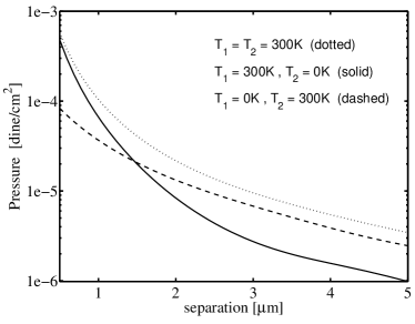
Figure 2: Thermal component (only $l$-dependent part) of the pressure out of equilibrium for fused silica-silicon system in the configuration ($T_{1}=300$K, $T_{2}=0$K) [solid] and in the configuration ($T_{1}=0$K, $T_{2}=300$K) [dashed]. We plot also the thermal part of the force at thermal equilibrium at $T=300$K [dotted].

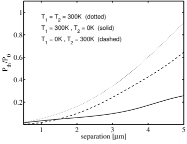
Figure 3: Relative contribution of the thermal component of the pressure (only $l$-dependent part) out of equilibrium for fused silica-silicon system in the configuration ($T_{1}=300$K, $T_{2}=0$K) [solid], ($T_{1}=0$K, $T_{2}=300$K) [dashed], and at thermal equilibrium at $T=300$K [dotted].

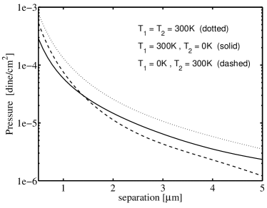
Figure 4: Same of Fig.2, for the sapphire-fused silica system.

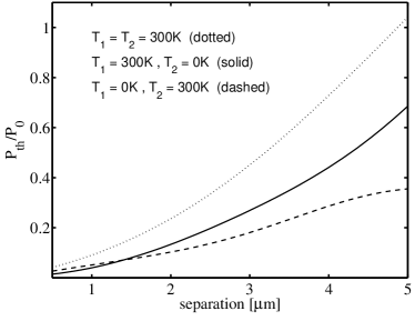
Figure 5: Same of Fig.3, for the sapphire-fused silica system.

VI Pressure between two thick slabs

In sections IV and V we derived and discussed the non-equilibrium pressure between two materials filling two infinite half-spaces. We did not regularized the pressure, i.e. we did not considered the extra-pressure due to the presence of the external surfaces of the bodies. This would simply add new $l$-independent terms. We focused mainly on the $l$-dependent part. In this section we fill this gap, and derive the exact constant terms of the pressure for the general case of two bodies of finite thicknesses at different temperatures, in presence of external radiation.

At thermal equilibrium, due to the momentum’s conservation theorem, the pressure cannot contain constant terms. In fact both Eq.(43) and (44) go to zero as $l$ goes to infinity. Here the regularization was performed by subtracting the bulk part of the full Green function [see discussion after Eq.(24)]. The inclusion of the bulk part would add an extra $l$-independent term $-4\sigma T^{4}/3c$, as it is evident from the non regularized Eq. (68). Physically the origin of this extra-term is due to the fact that the bodies are considered to be infinite, and hence, have no external surfaces. The presence of the external surfaces generates an extra pressure $4\sigma T^{4}/3c$, and finally the total pressure becomes $l$-independent. It is worth noticing that at thermal equilibrium the force acting on one body is exactly the same (apart from the sign) of that acting on the second body.

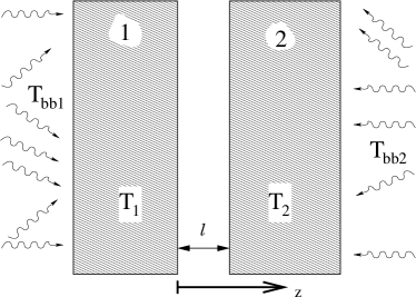
Figure 6: Schematic figure of the two-slab system out of thermal equilibrium.

Out of thermal equilibrium, for bodies occupying two half-spaces, one finds the non-regularized pressure given by the sum of Eqs.  (62) and (63). In this case the pressure contains distance-independent components, and is the same on both materials (apart from the sign). For bodies of finite thickness one should account for extra $l$-independent terms in the pressure due to the presence of two more interfaces between the bodies and the external regions (see Fig.6) where, in general, the radiation is not in equilibrium with the bodies. In this configuration the pressure acting on the body $1$ can be different from that acting on the body $2$. It should be noted that the new $l-$independent terms should be added to (70) and (71), and originate from the PW waves only. Below we derive the result for such a general configuration, by manipulating Eq. (62).

Let us consider the case where both the bodies occupy thick slabs, as represented in Fig.6. On the left of the body $1$ impinges radiation at temperature $T_{bb1}$, while on the right of the body $2$ impinges radiation at temperature $T_{bb2}$. Then the pressure acting on the body $1$ and body $2$ will be respectively:

$$\!\!\!\!\!\!\!\!\!P_{1,\textrm{th}}^{\textrm{neq}}(T_{bb1},T_{1},T_{2},l)\!\!\! = \!\!\!P_{\textrm{th}}^{\textrm{neq}}(T_{1},T_{2},l)+P_{\textrm{L}}(T_{1},T_{bb1}),$$ (76)

$$\!\!\!\!\!\!\!\!\!P_{2,\textrm{th}}^{\textrm{neq}}(T_{1},T_{2},T_{bb2},l)\!\!\! = \!\!\!-P_{\textrm{th}}^{\textrm{neq}}(T_{1},T_{2},l)+P_{\textrm{R}}(T_{2},T_{bb2}).$$ (77)

Here $P_{\textrm{th}}^{\textrm{neq}}(T_{1},T_{2},l)$ is the pressure out of thermal equilibrium given by the sum of (62) and (63) for materials filling infinite half-spaces. $P_{\textrm{L}}$ is the pressure due to the presence of a new left-side interface of the material $1$ while $P_{\textrm{R}}$ is the pressure due to the presence of a new right-side interface of the material $2$. Both $P_{\textrm{L}}$ and $P_{\textrm{R}}$ are constant terms and include two contributions: the pressure of the external radiation impinging on the outer interface and the back reaction produced by the emission of radiation from the body to the vacuum half-space.

For thick enough slabs, it is possible to calculate the terms $P_{\textrm{L}}$ and $P_{\textrm{R}}$ using the expression of the pressure acting on a body $h$ which occupies an infinite half-space. In general it has a dielectric function $\varepsilon_{h}$, is at temperature $T_{h}$, and a thermal radiation with temperature $T_{bb}$ impinges on its free surface. There are two possible configurations. One corresponds to the body $h$ on the left and radiation impinging from the right, the second correspond to the body on the right and radiation impinging from the left. In the two cases the pressures can be expressed in terms of the pressure between two infinite bodies $P_{\textrm{th}}^{\textrm{neq,PW}}(T_{1},T_{2},l)$ derived in the previous section, and are respectively:

$$\!\!\!\!\!\!P_{\textrm{R}}(T_{h},T_{bb})=$$ (78)

$$\!\!\!\!\!\!\left[P_{\textrm{th}}^{\textrm{neq,PW}}(0,T_{bb},l)+P_{\textrm{th}}^{\textrm{neq,PW}}(T_{h},0,l)\right]\Big{|}_{\varepsilon_{2}=1}^{\varepsilon_{1}\equiv\varepsilon_{h}},$$

$$\!\!\!\!\!\!P_{\textrm{L}}(T_{h},T_{bb})=$$ (79)

$$\!\!\!\!\!\!-\left[P_{\textrm{th}}^{\textrm{neq,PW}}(T_{bb},0,l)+P_{\textrm{th}}^{\textrm{neq,PW}}(0,T_{h},l)\right]\Big{|}_{\varepsilon_{1}=1}^{\varepsilon_{2}\equiv\varepsilon_{h}}.$$

Here $P_{\textrm{th}}^{\textrm{neq,PW}}(T,0,l)$ and $P_{\textrm{th}}^{\textrm{neq,PW}}(0,T,l)$ are given by Eq.(62). After explicit calculations one find

$$P_{\textrm{th}}^{\textrm{neq,PW}}(0,T_{bb},l)\Big{|}_{\varepsilon_{2}=1}^{\varepsilon_{1}\equiv\varepsilon_{h}} = -\frac{2\sigma T_{bb}^{4}}{3c}-P_{d}(T_{bb}),$$ (80)

$$P_{\textrm{th}}^{\textrm{neq,PW}}(T_{h},0,l)\Big{|}_{\varepsilon_{2}=1}^{\varepsilon_{1}\equiv\varepsilon_{h}} = -\frac{2\sigma T_{h}^{4}}{3c}+P_{d}(T_{h}),$$ (81)

where

$$P_{d}(T)=\frac{\hbar}{4\pi^{2}}\int_{0}^{\infty}\textrm{d}\omega\frac{1}{e^{\hbar\omega/k_{B}T}-1}\int_{0}^{k}\textrm{d}QQq_{z}\sum_{\mu=s,p}|r^{\mu}_{h}|^{2},$$ (82)

and $r^{\mu}_{h}$ are defined similar to (35) but using the dielectric function $\varepsilon_{h}$. Finally, we obtain the main result of this section, i.e. Eq.(78) becomes

$$P_{\textrm{R}}(T_{h},T_{bb})=-\frac{2\sigma(T_{h}^{4}+T_{bb}^{4})}{3c}+P_{d}(T_{h})-P_{d}(T_{bb}).$$ (83)

In the same way it is possible to calculate $P_{\textrm{L}}(T_{h},T_{bb})$ from Eq.(79), and it is evident that the result will be

$$P_{\textrm{L}}(T_{h},T_{bb})=-P_{\textrm{R}}(T_{h},T_{bb}).$$ (84)

At equilibrium $T_{h}=T_{bb}=T$ we find that $P_{\textrm{R}}(T,T)=-P_{\textrm{L}}(T,T)=-4\sigma T^{4}/3c$ does not depend on material characteristics and coincides with the pressure of the black body radiation. It is also interesting to see that for a white-body (W), corresponding to $|r^{\mu}_{h}|^{2}=1$, and for a black-body (B), corresponding to $|r^{\mu}_{h}|^{2}=0$, one obtains

$$P_{\textrm{R}}(0,T)_{\textrm{W}}=-\frac{4\sigma T^{4}}{3c}, P_{\textrm{R}}(0,T)_{\textrm{B}}=-\frac{2\sigma T^{4}}{3c},$$ (85)

$$P_{\textrm{R}}(T,0)_{\textrm{W}}=0, P_{\textrm{R}}(T,0)_{\textrm{B}}=-\frac{2\sigma T^{4}}{3c},.$$ (86)

From these relations one can see that $P_{\textrm{R}}(0,T)_{\textrm{W}}/P_{\textrm{R}}(0,T)_{\textrm{B}}=2$, as it should be for the radiation pressure. Furthermore one has that that $P_{\textrm{R}}(T,0)_{\textrm{W}}=0$. This is the consequence of the fact that if $|r^{\mu}_{h}|^{2}=1$ the radiation impinging on the surface from the interior of the material is fully reflected and there is no flux of momentum outside the body.

In the particular case when the external radiation is at equilibrium with the corresponding body, i.e. $T_{bb1}=T_{1}$ and $T_{bb2}=T_{2}$, from (83) and (84) one obtains that Eqs. (76) and (77) become respectively

$$\!\!\!\!\!\!\!\!P_{1,\textrm{th}}^{\textrm{neq}}(T_{bb1}=T_{1},T_{1},T_{2},l)\!\! = \!\!P_{\textrm{th}}^{\textrm{neq}}(T_{1},T_{2},l)+\frac{4\sigma T_{1}^{4}}{3c},$$ (87)

$$\!\!\!\!\!\!\!\!P_{2,\textrm{th}}^{\textrm{neq}}(T_{1},T_{2},T_{bb2}=T_{2},l)\!\! = \!\!-P_{\textrm{th}}^{\textrm{neq}}(T_{1},T_{2},l)-\frac{4\sigma T_{2}^{4}}{3c}.$$ (88)

If the whole system is at thermal equilibrium, $T_{1}=T_{2}=T$, the last two equations give

$$\!\!\!\!\!\!\!\!P_{1,\textrm{th}}^{\textrm{neq}}(T,T,T,l)=-P_{2,\textrm{th}}^{\textrm{neq}}(T,T,T,l)=$$ (89)

$$P_{\textrm{th}}^{\textrm{neq}}(T,T,l)+\frac{4\sigma T^{4}}{3c}=P_{\textrm{th}}^{\textrm{eq}}(T,l).$$

This reproduces Eq.(68), where $P_{\textrm{th}}^{\textrm{neq}}(T,T,l)\equiv\overline{P}_{\textrm{th}}^{\textrm{eq,PW}}(T,l)$.

VII Long distance behavior of the surface-surface pressure

Let us consider now the surface-surface pressure in the limit of large separation. In this limit the relevant frequencies are $\omega\simeq c/l\ll k_{B}T/\hbar$. If this frequency is smaller than the lowest absorption resonance in the material, one can use the static approximation for the dielectrics and change $\varepsilon_{i}(\omega)\rightarrow\varepsilon_{0i}$. Some dielectrics can have very low-lying resonances. For this case we developed a special procedure that will be discussed later.

At thermal equilibrium the pressure is given by Eqs.(43) and (44) for the PW and EW components, respectively. In the limit of large distances these components behave as AntezzaPhDthesis

$$\!\!\!\!\!\!\!\!P_{\textrm{th}}^{\textrm{eq,PW}}(T,l) = \frac{k_{B}T\zeta(3)}{4\pi l^{3}},$$ (90)

$$\!\!\!\!\!\!\!\!P_{\text{th}}^{\text{eq,EW}}(T,l) = -\frac{k_{B}T\zeta(3)}{4\pi l^{3}}+$$ (91)

$$\!\!\!\!\!\!\!\!\!\!\!\!\!\!\!\!\!\!\!\!\!\!\!\!\!\!\!\!\!\!\!\!\!\!\!\!\!\frac{k_{B}T}{16\pi l^{3}}\int_{0}^{\infty}\text{d}x\;x^{2}\left[\frac{\varepsilon_{10}+1}{\varepsilon_{10}-1}\frac{\varepsilon_{20}+1}{\varepsilon_{20}-1}\;e^{x}-1\right]^{-1},$$

where $\zeta(3)\approx 1.2021$ is the Riemann zeta-function. These equations are both valid at the condition

$$l\gg\textrm{max}_{m=1,2}\left(\frac{\varepsilon_{m0}}{\sqrt{\varepsilon_{m0}-1}}\right)\lambda_{T},$$ (92)

where $\lambda_{T}$ is defined in Eq.(42). The first term in Eq. (91) is canceled by the contribution from the propagating waves (90), and their sum provides the well known result for the total force at equilibrium (46). It is worth noticing that the total force at equilibrium is valid at the condition (45), which is significantly different from (92) if one of the two bodies is rarefied.

The surface-surface force in the non-equilibrium case is given by Eqs. (70) and (71). Omitting the $l$-independent terms one finds for the large distance behavior the following result ShortArticle :

$$P_{\textrm{th}}^{\textrm{neq,PW}}(T,0,l) = \frac{k_{B}T\zeta(3)}{16\pi l^{3}}\left[2-\frac{\sqrt{\varepsilon_{10}-1}-\sqrt{\varepsilon_{20}-1}}{\sqrt{\varepsilon_{10}-1}+\sqrt{\varepsilon_{20}-1}}-\frac{\varepsilon_{20}\sqrt{\varepsilon_{10}-1}-\varepsilon_{10}\sqrt{\varepsilon_{20}-1}}{\varepsilon_{20}\sqrt{\varepsilon_{10}-1}+\varepsilon_{10}\sqrt{\varepsilon_{20}-1}}\right],$$ (93)

$$P_{\textrm{th}}^{\textrm{neq,EW}}(T,0,l) = \frac{k_{B}T}{8\pi^{2}l^{3}}\int_{0}^{\infty}\textrm{d}t\int_{0}^{\infty}\textrm{d}x\;\frac{x^{2}\;e^{-x}}{t}\;\sum_{\mu=s,p}\;\frac{\textrm{Im}\left[r^{\mu}_{1}(t)\right]\textrm{Re}\left[r^{\mu}_{2}(t)\right]}{|1-r^{\mu}_{1}(t)r^{\mu}_{2}(t)\;e^{-x}|^{2}}.$$ (94)

Here $r^{\mu}_{m}(t)$ are the Fresnel reflection coefficients (35) in the static approximation $\varepsilon_{m}=\varepsilon_{m0}$, and $t$ is defined by the relation $Q^{2}=k^{2}\left(1+t^{2}\right)$. Note that the equations (93) and (94) are also valid at the condition (92).

In the two following subsections VII.1 and VII.2 we will describe the procedure we used to calculate the large distance asymptotic behaviors (93) and (94) for the PW and EW components, respectively.

VII.1 Asymptotic behavior for PW

In this subsection we derive the expansion of the PW contribution $P_{\textrm{th}}^{\textrm{neq,PW}}(T,0,l)$ at large distances, just anticipated in Eq. (93). We concentrate on the $l$-dependent part only. One can start from Eq. (62). It is helpful to use the multiple-reflection expansion expressed by Eq. (69). The first term in this expansion corresponds to radiation which is emitted by one plate and absorbed by the other one, without being reflected back. This is a distance independent term which we omit. All the other terms of the sum give contribution to the distance dependent part to which we are interested.

Let us introduce new variables and parameters in Eq. (62), i.e.

$$x=\frac{\hbar\omega}{k_{B}T},\;Q^{2}=k^{2}(1-t^{2}),\;\alpha=\frac{\lambda_{T}}{2l}.$$ (95)

The limit of large distances corresponds to $\alpha\ll 1$. In terms of these new variables one finds

$$P_{\textrm{th}}^{\textrm{neq,PW}}(T,0,l)=\frac{(k_{B}T)^{4}}{2\pi^{2}\hbar^{3}c^{3}}\sum_{n=1}^{\infty}\textrm{Re}\left\{\int_{0}^{\infty}\textrm{d}x\frac{x^{3}}{e^{x}-1}\int_{0}^{1}\textrm{d}tt^{2}\sum_{\mu=s,p}\frac{\left(1-\left|r^{\mu}_{1}\right|^{2}\right)\left(1+\left|r^{\mu}_{2}\right|^{2}\right)}{1-\left|r^{\mu}_{1}r^{\mu}_{2}\right|^{2}}\;\left(r^{\mu}_{1}r^{\mu}_{2}\right)^{n}\;e^{intx/\alpha}\right\},$$ (96)

where the reflection coefficients as functions of $x$ and $t$ are

$$r^{s}_{m}(t,x) = \frac{t-\sqrt{\varepsilon_{m}-1+t^{2}}}{t+\sqrt{\varepsilon_{m}-1+t^{2}}},$$ (97)

$$r^{p}_{m}(t,x) = \frac{\varepsilon_{m}t-\sqrt{\varepsilon_{m}-1+t^{2}}}{\varepsilon_{m}t+\sqrt{\varepsilon_{m}-1+t^{2}}},$$ (98)

and $\varepsilon_{m}=\varepsilon_{m}(k_{B}Tx/\hbar)$ is a function of the variable $x$. For $\alpha\ll 1$ the integrand in (96) oscillates fast and it is possible to show that the relevant values of variables in the integral are $x\lesssim 1$ and $t\sim\alpha/n$. Then, expanding the reflection coefficients for small values of $t$ and integrating over $t$ explicitly one finds the leading term in $\alpha$

$$\!\!\!\!\!\!P_{\textrm{th}}^{\textrm{neq,PW}}(T,0,l)=$$ (99)

$$\!\!\!\!\frac{k_{B}T}{8\pi^{2}l^{3}}\sum_{n=1}^{\infty}\frac{1}{n^{3}}\int_{0}^{\infty}\textrm{d}x\frac{\sin(nx/\alpha)}{e^{x}-1}\sum_{\mu=s,p}g_{\mu}(x),$$

where the following functions of $x$ were introduced

$$g_{s}\left(x\right)=\frac{2\textrm{Re}\left(\beta_{1}\right)}{\textrm{ Re}\left(\beta_{1}+\beta_{2}\right)},\;\;g_{p}\left(x\right)=\frac{2\textrm{ Re}\left(\gamma_{1}\right)}{\textrm{ Re}\left(\gamma_{1}+\gamma_{2}\right)},$$ (100)

with

$$\beta_{m}(x)=\frac{1}{\sqrt{\varepsilon_{m}-1}},\;\;\gamma_{m}(x)=\frac{\varepsilon_{m}}{\sqrt{\varepsilon_{m}-1}}.$$ (101)

The leading contribution to $P_{\textrm{th}}^{\textrm{neq,PW}}(T,0,l)$ comes from the region $x\sim\alpha/n\ll 1$, where $e^{x}-1\approx x$. Note that one can do this expansion only after explicit integration over $t$. After the change of variable $y=nx/\alpha$ we obtain

$$\!\!\!\!\!\!P_{\textrm{th}}^{\textrm{neq,PW}}(T,0,l)=$$ (102)

$$\!\!\!\!\frac{k_{B}T}{8\pi^{2}l^{3}}\sum_{n=1}^{\infty}\frac{1}{n^{3}}\int_{0}^{\infty}\textrm{d}y\frac{\sin y}{y}\sum_{\mu=s,p}g_{\mu}(\alpha y/n).$$

The relevant range of integration here is $y\sim 1$, and then the important frequencies in the dielectric functions entering in Eq.(101) are of the order of $\hbar\omega\sim\alpha k_{B}T$. Most of the dielectrics (but not all) at these frequencies have no dispersion in the spectrum and one can take the static approximation $g_{\mu}\left(\alpha y/n\right)\approx g_{\mu}\left(0\right)$. In this case the integral in Eq. (102) can be calculated explicitly:

$$P_{\textrm{th}}^{\textrm{neq,PW}}(T,0,l)=\frac{k_{B}T}{16\pi l^{3}}\zeta(3)\left[g_{s}(0)+g_{p}(0)\right],$$ (103)

where

$$g_{s}\left(0\right) = \frac{2\sqrt{\varepsilon_{20}-1}}{\sqrt{\varepsilon_{10}-1}+\sqrt{\varepsilon_{20}-1}},$$ (104)

$$g_{p}\left(0\right) = \frac{2\varepsilon_{10}\sqrt{\varepsilon_{20}-1}}{\varepsilon_{20}\sqrt{\varepsilon_{10}-1}+\varepsilon_{10}\sqrt{\varepsilon_{20}-1}}.$$ (105)

Eq. (103) coincides with (93) after elementary transformation. This expression is valid under the condition (92) that justify the expansion on $t$ done for the reflection coefficients (97) and (98).

It is interesting to derive also the large distance behavior (90) for the equilibrium case. To do this we can note that the symmetric part of the non-equilibrium pressure in respect to the interchange of the bodies coincides with one half of the equilibrium pressure as Eq. (70) demonstrates. The symmetric part of both $g_{s}(x)$ and $g_{p}(x)$ is equal to 1 and we immediately reproduce the result (90).

VII.2 Asymptotic behavior for EW

In this subsection we show how to evaluate the asymptotic behavior of the EW contribution to the pressure $P_{\textrm{th}}^{\textrm{neq,EW}}(T,0,l)$, whose result was anticipated in Eq.(94). We start from the general expression for $P_{\textrm{th}}^{\textrm{neq,EW}}(T,0,l)$ given by Eq. (63). Substituting in this equation $x$ and $\alpha$ given by (95), but defining $t$ as $Q^{2}=k^{2}\left(1+t^{2}\right)$, one finds for the pressure

$$\!\!\!\!\!\!\!\!\!\!\!\!P_{\textrm{th}}^{\textrm{neq,EW}}(T,0,l)=\frac{(k_{B}T)^{4}}{\pi^{2}\hbar^{3}c^{3}}\int_{0}^{\infty}\textrm{d}x\frac{x^{3}}{e^{x}-1}\times$$ (106)

$$\!\!\!\!\int_{0}^{\infty}\textrm{d}tt^{2}e^{-xt/\alpha}\;\sum_{\mu=s,p}\frac{\textrm{Im}\left(r^{\mu}_{1}\right)\textrm{Re}\left(r^{\mu}_{2}\right)}{|1-r^{\mu}_{1}r^{\mu}_{2}\;e^{-xt/\alpha}|^{2}}.$$

Here the reflection coefficients are functions of $t$ and $x$ and take the form

$$r^{s}_{m}(t,x) = \frac{it-\sqrt{\varepsilon_{m}-1-t^{2}}}{it+\sqrt{\varepsilon_{m}-1-t^{2}}},$$ (107)

$$r^{p}_{m}(t,x) = \frac{i\varepsilon_{m}\;t-\sqrt{\varepsilon_{m}-1-t^{2}}}{i\varepsilon_{m}\;t+\sqrt{\varepsilon_{m}-1-t^{2}}},$$ (108)

with $\varepsilon_{m}=\varepsilon_{m}(k_{B}Tx/\hbar)$.

Differently from the PW component, here the relevant ranges of variables in the integral (106) are $x\sim\alpha$ and $t\sim 1$. Small values of $t$ do not give significant contribution because the integrand is suppressed by a factor $t$ coming from $\textrm{Im}\left(r^{\mu}_{1}\right)$, that do not appears in the PW case. Then for large distances it is possible to expand on small values of $x$ and approximate $e^{x}-1\approx x$. It is convenient to introduce the new variable $y=xt/\alpha$ instead of $x$, for which the important range is now $y\sim 1$. In terms of $y$ and $t$ the pressure can be presented as

$$\!\!\!\!\!\!\!\!\!\!\!\!P_{\textrm{th}}^{\textrm{neq,EW}}(T,0,l)=\frac{k_{B}T}{8\pi^{2}l^{3}}\int_{0}^{\infty}\frac{\textrm{d}t}{t}\times$$ (109)

$$\;\;\;\;\;\int_{0}^{\infty}\textrm{d}yy^{2}e^{-y}\sum_{\mu=s,p}\frac{\textrm{Im}\left(r^{\mu}_{1}\right)\textrm{Re}\left(r^{\mu}_{2}\right)}{|1-r^{\mu}_{1}r^{\mu}_{2}\;e^{-y}|^{2}}.$$

The relevant frequencies in the integration are $\omega\sim c/l\ll k_{B}T/\hbar$ and then it is possible to use the static approximation for the dielectric functions. In this approximation the reflection coefficients depends only on one variable $r^{\mu}_{1,2}(t,y)\rightarrow r^{\mu}_{1,2}(t)$ and one can reproduce (after the change $y\rightarrow x$) the asymptotic behavior (94) for the pressure $P_{\textrm{th}}^{\textrm{EW}}(T,0,l)$ .

The pressure in the EW sector can be presented in an alternative form using the multiple-reflection expansion. To this end one can note that

$$\frac{e^{-xt/\alpha}}{|1-r^{\mu}_{1}r^{\mu}_{2}\;e^{-xt/\alpha}|^{2}}=\sum_{n=1}^{\infty}\frac{\textrm{Im}(r^{\mu}_{1}r^{\mu}_{2})^{n}}{\textrm{Im}(r^{\mu}_{1}r^{\mu}_{2})}\;e^{-nxt/\alpha},$$ (110)

and can put this expansion in Eq. (106). In the static approximation the integral over $x$ can be found explicitly:

$$\int_{0}^{\infty}\textrm{d}x\frac{x^{3}}{e^{x}-1}\;e^{-nxt/\alpha}=\Psi^{(3)}\left(1+nt/\alpha\right),$$ (111)

where $\Psi^{(3)}\left(1+nt/\alpha\right)$ is the polygamma function Abram . Since $\alpha$ is small, one can take only the asymptotic of this function, which is $\Psi^{(3)}\left(1+nt/\alpha\right)\rightarrow 2(\alpha/nt)^{3}$. Then the EW pressure can be presented as

$$\!\!\!\!\!\!\!\!\!\!\!\!\!P_{\textrm{th}}^{\textrm{neq,EW}}(T,0,l)=\frac{k_{B}T}{4\pi^{2}l^{3}}\sum_{n=1}^{\infty}\frac{1}{n^{3}}\int_{0}^{\infty}\frac{\textrm{d}t}{t}\times$$ (112)

$$\;\;\;\;\;\;\;\;\;\sum_{\mu=s,p}\frac{\textrm{Im}\left(r^{\mu}_{1}\right)\textrm{Re}\left(r^{\mu}_{2}\right)}{\textrm{Im}\left(r^{\mu}_{1}r^{\mu}_{2}\right)}\textrm{Im}\left(r^{\mu}_{1}r^{\mu}_{2}\right)^{n}.$$

This representation is helpful for the analysis of the rarefied body limit that will be presented in the next section.

It is interesting to derive also the large distance behavior (91) for the equilibrium case. One half of the equilibrium pressure, $P^{\textrm{eq,EW}}_{\textrm{th}}(T,l)/2$, is equal to the symmetric part of Eq. (112) in respect to the bodies interchange. Therefore, to get $P^{\textrm{eq,EW}}_{\textrm{th}}(T,l)$ we have to change in Eq. (112):

$$\frac{\textrm{Im}\left(r^{\mu}_{1}\right)\textrm{Re}\left(r^{\mu}_{2}\right)}{\textrm{Im}\left(r^{\mu}_{1}r^{\mu}_{2}\right)}\rightarrow 1.$$ (113)

In this case the integrand in Eq. (112) becomes an analytic function of $t$ with the poles at $t=0$ and at infinity. The integral can be calculated using the quarter-circle contour of infinite radius closing the positive real axis and negative imaginary axis. This is because $it\sim q_{z}$ must have a positive real part. Finally the integral is reduced to the quarters of the residues in the poles and gives:

$$\!\!\!\!\!\!\!\!\!\!\!P^{\textrm{eq,EW}}_{\textrm{th}}(T,l)=-\frac{k_{B}T\zeta(3)}{4\pi l^{3}}+$$ (114)

$$\;\;\;\;\;\;\;\frac{k_{B}T}{8\pi l^{3}}\sum_{n=1}^{\infty}\frac{1}{n^{3}}\left(\frac{\varepsilon_{10}-1}{\varepsilon_{10}+1}\frac{\varepsilon_{20}-1}{\varepsilon_{20}+1}\right)^{n}.$$

The sum in this expression can be written in the equivalent integral form so that (114) coincides with Eq. (91). Note that only $p$-polarization contributes to the pole at infinity. This is because at infinity $r^{s}_{m}\rightarrow 0$ but $r^{p}_{m}\rightarrow(\varepsilon_{m0}-1)/(\varepsilon_{m0}+1)$ stays finite.

VIII Pressure between a solid and a diluted body

A case of particular interest is the interaction between solid and diluted bodies. In fact the first measurement of the non-equilibrium interaction was done between an ultracold atomic cloud and a dielectric substrate Cornell06 . From the theoretical point of view this case is the most simple for analytical analysis.

Here we investigate the pressure between a hot dielectric substrate of temperature $T$ (body 1) and a gas cloud (body 2) at large distances. When the second body is very dilute we can consider the limit $(\varepsilon_{2}-1)\rightarrow 0$. If both bodies are at the same temperature $T$, the equilibrium pressure can be found by expanding Eq. (46) on small values of $(\varepsilon_{2}-1)$. The leading term is

$$P_{\textrm{th}}^{\textrm{eq}}(T,l)=\frac{k_{B}T}{16\pi l^{3}}\frac{\varepsilon_{10}-1}{\varepsilon_{10}+1}\;(\varepsilon_{20}-1).$$ (115)

This pressure, valid at the condition (45), is proportional to $(\varepsilon_{2}-1)=4\pi n\alpha$, where $n$ is the density of the material $2$ and $\alpha$ is the dipole polarizability of its constituents (for example atoms). We can see that the pressure is additive since the additivity would in fact require a linear dependence on the gas density $n$ and hence on $(\varepsilon_{20}-1)$.

If one performs first the diluteness limit of the exact surface-surface pressure, and then takes the large distance limit, one obtains very interesting asymptotic behaviors for the PW and EW contributions respectively AntezzaPhDthesis

$$\!\!\!P_{\textrm{th}}^{\textrm{eq,PW}}(T,l) = -\frac{(k_{B}T)^{2}}{24\;l^{2}\;c\hbar}\frac{\varepsilon_{10}+1}{\sqrt{\varepsilon_{10}-1}}\;(\varepsilon_{20}-1),$$ (116)

$$\!\!\!P_{\textrm{th}}^{\textrm{eq,EW}}(T,l) = \frac{(k_{B}T)^{2}}{24\;l^{2}\;c\hbar}\frac{\varepsilon_{10}+1}{\sqrt{\varepsilon_{10}-1}}\;(\varepsilon_{20}-1).$$ (117)

In deriving these limits we assumed that $k_{B}T$ is much smaller than the lowest dielectric resonance of both the body $1$ and of the atoms of the dilute body $2$. Such asymptotic behaviors for the PW and EW components depend on the temperature more strongly than at equilibrium and decay slower at large distances ($\sim T^{2}/l^{2}$). It is also remarkable that the PW component of the surface-rarefied body pressure (116) depends on the dielectric functions and is repulsive, differently from attractive nature of the PW component of the surface-surface pressure (90).

The PW and EW terms (116) and (117) exactly cancel each other, and in order to find the total pressure one should expand the corresponding expressions to higher order. The final result is given by Eq. (115). In configurations out of thermal equilibrium there will be no longer such peculiar cancellations between the PW and EW terms. In this case the new asymptotic behavior $\sim T^{2}/l^{2}$ will characterize the total pressure at large distances, while there will be a transition to a $\sim T/l^{3}$ behavior at larger distances.

In particular, the result of the surface-rarefied body pressure out of equilibrium can be presented as ShortArticle

$$P^{\textrm{neq}}_{\textrm{th}}(T,0,l)=\frac{k_{B}TC}{l^{3}}\frac{\varepsilon_{10}+1}{\sqrt{\varepsilon_{10}-1}}\sqrt{\varepsilon_{20}-1}f(v),$$ (118)

where

$$v=\frac{l\sqrt{\varepsilon_{20}-1}}{\lambda_{T}}$$ (119)

is a dimensionless variable and $C=3.83\cdot 10^{-2}$ is a constant. The function $f(v)$, whose expression will be derived below [see Eq.(149), together with Eqs. (131), (VIII.2), and (VIII.2)], is a dimensionless function of $v$. It is possible to show (see derivation below) that $f(v)\rightarrow 1$ for $v\rightarrow\infty$, while $f(v)\rightarrow v/24C$ for $v\rightarrow 0$. This function is shown in Fig. 7. Eq. (118) is valid at the condition of large distances $l/\lambda_{T}\gg 1$, which does not restrict the value of $v$.

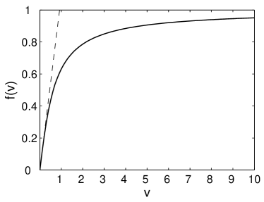
Figure 7: Dimensionless function $f(v)$ [see Eqs. (118) and (149] describing the transition between additive and nonadditive regimes. The dashed line presents the asymptotic limit at small $v$.

At large values of $v$ the pressure (118) becomes

$$P^{\textrm{neq}}_{\textrm{th}}(T,0,l)=\frac{k_{B}TC}{l^{3}}\frac{\varepsilon_{10}+1}{\sqrt{\varepsilon_{10}-1}}\sqrt{\varepsilon_{20}-1},$$ (120)

and is proportional to $\sqrt{\varepsilon_{20}-1}$. This peculiar dependence means that the pressure acting on the atoms of the substrate $2$ is not additive. The non additivity of the pressure can be physically explained as follow: for large $l$ the main contribution to the force is produced by the grazing waves incident on the interface of the material $2$ from the vacuum gap with small values of $q_{z}/k\leq\sqrt{\varepsilon_{20}-1}$. Hence the reflection coefficients from the body $2$ is not small even at small $\varepsilon_{20}-1$ and the body cannot be considered as dilute from an electrodynamic point of view ShortArticle . This is a peculiarity of the non-equilibrium situation. In fact at equilibrium this anomalous contribution is canceled by the waves impinging the interface from the interior of the dielectric $2$, close to the angle of total reflection. In a rarefied body such waves become grazing. Notice that the pressure (120) is valid at the condition

$$l\gg\frac{\lambda_{T}}{\sqrt{\varepsilon_{20}-1}},$$ (121)

which becomes stronger and stronger as $(\varepsilon_{20}-1)~{}\to~{}0$.

At small $v$ one finds from Eq.(118)

$$P^{\textrm{neq}}_{\textrm{th}}(T,0,l)=\frac{(k_{B}T)^{2}}{24l^{2}\hbar c}\frac{\varepsilon_{10}+1}{\sqrt{\varepsilon_{10}-1}}(\varepsilon_{20}-1).$$ (122)

In this case the additivity is restored but the temperature dependence is not linear any more and the pressure decreases more slowly with the distance. This result holds at distances

$$\lambda_{T}\ll l\ll\frac{\lambda_{T}}{\sqrt{\varepsilon_{20}-1}}.$$ (123)

It is worth noting that the interval (123) practically disappears for dense dielectrics.

The above discussion can be summarized as follow [see Fig.8]. If the dielectric $2$ is very dilute but still occupies an infinite half space (or anyway is thick enough, in the sense defined above), there is a first region given by Eq.(123) where the pressure is additive and coincides with Eq.(122). At larger distances, satisfying Eq.(121), the pressure is given by Eq.(120) and is no longer additive. In the intermediate region $l\sim\lambda_{T}/\sqrt{\varepsilon_{20}-1}$ equations (122) and (120) are of the same order.

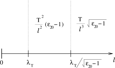
Figure 8: Relevant length scales and asymptotic behaviors of the surface-rarefied body pressure out of thermal equilibrium. There is a first region given by Eq.(123) where the pressure is additive and coincides with Eq.(122), and a second region, satisfying Eq.(121), where the pressure is given by Eq.(120) and is no longer additive.

It is interesting to note that, due to the diluteness condition $(\varepsilon_{20}-1)\ll 1$, in both regions (121) and (123) the thermal term $\Delta P_{\textrm{th}}$ [sum of Eqs.(73) and (75)] gives the leading contribution into the $l-$dependent component of the total pressure $P^{\textrm{neq}}_{\textrm{th}}(T,0,l)$. This clearly emerges from Eqs.(70) - (71), by comparing (fot $T_{2}=0$) the large distance behavior of the pressure at equilibrium $P^{\textrm{eq}}_{\textrm{th}}(T,l)$ given by Eq.(115), with the large distance behaviors of the total pressure just derived, given by Eqs.(120) and (122). The consequences of this are remarkable. In fact the large distance behavior of the total pressure becomes proportional to

$$P^{\textrm{neq}}_{\textrm{th}}(T_{1},T_{2},l)\simeq\Delta P_{\textrm{th}}(T_{1},l)-\Delta P_{\textrm{th}}(T_{2},l),$$

and the interaction between the two bodies will be attractive if $T_{1}>T_{2}$ and repulsive in the opposite case ShortArticle .

Below, in sections VIII.1 and VIII.2, we present the derivation of Eq.(118) for both the PW and EW components, which give rise respectively to the asymptotic behaviors (120) and (122).

VIII.1 PW contribution

In this section we focus on the PW contribution to Eq. (118). One can do explicit calculations if the dielectric functions of the materials do not depend on frequency. This is a good approximation for the diluted body 2. Since we are interested in the large distance asymptotic, this approximation is also good for the solid body 1 if the material has no resonances for $\omega<c/l\ll k_{B}T/\hbar$. In the case of static dielectric functions the integral over $x$ in Eq. (96) can be evaluated via the polygamma function:

$$\int_{0}^{\infty}\frac{\textrm{d}xx^{3}}{e^{x}-1}e^{intx/\alpha}=\Psi^{(3)}\left(1-i\frac{nt}{\alpha}\right).$$ (124)

Then, introducing the new variable $u$ instead of $t$ and the parameter $b$ according to the definitions

$$u=\frac{t}{\sqrt{\varepsilon_{20}-1}},\ \ \ b=\sqrt{\frac{\varepsilon_{10}-1}{\varepsilon_{20}-1}}\gg 1$$ (125)

one can expand $r_{1}^{\mu}(u)$ in series of $1/b$

$$r_{1}^{s}\approx-\left(1-\frac{2u}{b}\right),\ \ \ r_{1}^{p}\approx-\left(1-\frac{2\varepsilon_{1}u}{b}\right)$$ (126)

and in the same approximation one has

$$r_{2}^{p}\approx r_{2}^{s}=r_{2}=\frac{u-\sqrt{1+u^{2}}}{u+\sqrt{1+u^{2}}}.$$ (127)

The result is the following expression for the pressure $P_{\textrm{th}}^{\textrm{neq,PW}}(T,0,l)$:

$$P_{\textrm{th}}^{\textrm{neq,PW}}(T,0,l)=-\frac{2(k_{B}T)^{4}}{\pi^{2}\hbar^{3}c^{3}}\frac{\varepsilon_{10}+1}{\sqrt{\varepsilon_{10}-1}}(\varepsilon_{20}-1)^{2}\sum_{n=1}^{\infty}\times$$

$$\int_{0}^{1/\sqrt{\varepsilon_{20}-1}}\textrm{d}uu^{3}\frac{1+r_{2}^{2}}{1-r_{2}^{2}}(-r_{2})^{n}\textrm{Re}\Psi^{(3)}\left(1-i2nvu\right),$$

(128)

where the parameter $v$ is given by Eq. (119). Here the sum on polarizations gave the factor $\varepsilon_{10}+1$. In the leading approximation the integration over $u$ can be extended up to infinity. Furthermore, the real part of $\Psi^{(3)}\left(1-iy\right)$ can be presented as Abram

$$\textrm{Re}\Psi^{(3)}\left(1-iy\right)=\frac{\pi}{2}\frac{\textrm{d}^{3}}{\textrm{d}y^{3}}\left(\frac{1}{\pi y}-\coth\pi y\right).$$ (129)

After some transformations equation (128) becomes:

$$P_{\textrm{th}}^{\textrm{neq,PW}}(T,0,l)=\frac{k_{B}T}{l^{3}}\frac{\varepsilon_{10}+1}{\sqrt{\varepsilon_{10}-1}}\sqrt{\varepsilon_{20}-1}f_{PW}(v),$$ (130)

where $f_{PW}(v)$ is given by

$$\!\!\!\!\!\!\!\!\!\!\!\!\!\!\!\!\!\!\!\!\!\!\!\!f_{PW}(v)=-\frac{1}{8\pi}\sum_{n=1}^{\infty}\frac{1}{n^{3}}\int_{0}^{\infty}\textrm{d}uu^{3}\frac{1+r_{2}^{2}}{1-r_{2}^{2}}(-r_{2})^{n}\times$$ (131)

$$\!\!\!\frac{\textrm{d}^{3}}{\textrm{d}u^{3}}\left[\frac{1}{2\pi nvu}-\coth(2\pi nvu)\right].$$

The function $f_{PW}(v)$ can be calculated explicitly for large and small values of $v$. When $v\gg 1$, the important range of $u$ in the integral (131) is $u\ll 1$ and one can expand the reflection coefficient $r_{2}$ on small values of $u$. Then the function $f_{PW}(v)$ is reduced to

$$\!\!\!\!\!\!\!\!\!\!\!\!\!\!\!\!\!\!\!\!\!\!\!\!f_{PW}(v\rightarrow\infty)=-\frac{1}{16\pi}\sum_{n=1}^{\infty}\frac{1}{n^{3}}\int_{0}^{\infty}\textrm{d}uu^{2}\times$$ (132)

$$\!\!\!\frac{\textrm{d}^{3}}{\textrm{d}u^{3}}\left[\frac{1}{2\pi nvu}-\coth(2\pi nvu)\right].$$

The integral here is easily calculated by parts and finally one finds

$$f_{PW}(v\rightarrow\infty)=C_{PW}=\frac{\zeta(3)}{8\pi}.$$ (133)

When $v\ll 1$ the significant values of $u$ in the integral (131) are $u\gg 1$, and one can make the corresponding expansion in the reflection coefficient (127). In this case only the $n=1$ term in the sum is relevant. Then one obtains

$$\!\!\!\!\!\!\!\!\!\!\!\!\!\!\!\!\!\!f_{PW}(v\rightarrow 0)=-\frac{1}{32\pi}\int_{0}^{\infty}\textrm{d}uu\times$$ (134)

$$\!\!\!\!\!\!\frac{\textrm{d}^{3}}{\textrm{d}u^{3}}\left[\frac{1}{2\pi vu}-\coth(2\pi vu)\right],$$

and finally:

$$f_{PW}(v\rightarrow 0)=\frac{v}{48}.$$ (135)

The function $f_{PW}(v)$ and its asymptotic behaviours at large and small $v$ are shown in Fig.9.

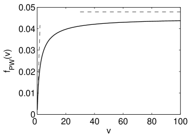
Figure 9: Function $f_{PW}(v)$ (solid) [Eq.(131)] and its asymptotic limits (dashed) at small [Eq.(135)] and large [Eq.(133)] values of $v$.

VIII.2 EW contribution

The derivation of the EW component of the pressure (118) can be performed starting from the expression (106) for the pressure $P_{\textrm{th}}^{\textrm{neq,EW}}(T,0,l)$. By performing the multiple-reflection expansion with the help of Eq. (110) and calculating the integral over the variable $x$ using (111) one finds that Eq.(106) becomes

$$\!\!\!\!\!\!\!P_{\textrm{th}}^{\textrm{neq,EW}}(T,0,l)=\frac{(k_{B}T)^{4}}{\pi^{2}\hbar^{3}c^{3}}\sum_{n=1}^{\infty}\int_{0}^{\infty}\textrm{d}tt^{2}\times$$ (136)

$$\sum_{\mu=s,p}\frac{\textrm{Im}r_{1}^{\mu}\textrm{Re}r_{2}^{\mu}}{\textrm{Im}(r_{1}^{\mu}r_{2}^{\mu})}\textrm{Im}(r_{1}^{\mu}r_{2}^{\mu})^{n}\Psi^{(3)}\left(1+\frac{nt}{\alpha}\right),$$

As in the case of the propagating waves one can introduce the variable $u$ instead of $t$ according to Eq. (125), and can make the expansion for large $b$. Then for the reflection coefficients one gets

$$r_{1}^{s}\approx-\left(1-\frac{i2u}{b}\right),\ \ \ r_{1}^{p}\approx-\left(1-\frac{i2\varepsilon_{1}u}{b}\right)$$

$$r_{2}^{p}\approx r_{2}^{s}=\frac{iu-\sqrt{1-u^{2}}}{iu+\sqrt{1-u^{2}}}.\ \ \ \ \ \ \ \ \ \$$ (137)

Now one should distinct the integration ranges $0<u<1$ and $1<u<\infty$, since the integrands are different in these ranges. Let us do it with the superscript $(1)$ or $(2)$, respectively.

As in the case of propagating waves (130) the pressure can be presented as a parameter-dependent factor times a universal function of $v=l\sqrt{\varepsilon_{20}-1}/\lambda_{T}$:

$$P_{\textrm{th}}^{\textrm{neq,EW}}(T,0,l)=\frac{k_{B}T}{l^{3}}\frac{\varepsilon_{10}+1}{\sqrt{\varepsilon_{10}-1}}\sqrt{\varepsilon_{20}-1}f_{EW}(v),$$ (138)

where the function $f_{EW}(v)$ includes contributions from $0<u<1$ and $1<u<\infty$ ranges:

$$f_{EW}(v)=f_{EW}^{(1)}(v)+f_{EW}^{(2)}(v).$$ (139)

For these functions one has the following expressions

$$\!\!\!\!\!\!\!\!\!\!f_{EW}^{(1)}(v)=-\frac{1}{4\pi^{2}}\sum_{n=1}^{\infty}\frac{1}{n^{3}}\int_{0}^{1}\textrm{d}uu^{3}\times$$

$$\frac{2u^{2}-1}{2u\sqrt{1-u^{2}}}\textrm{Im}(-r_{2})^{n}\frac{\textrm{d}^{3}}{\textrm{d}u^{3}}\Psi\left(1+2nvu\right);$$ (140)

$$f_{EW}^{(2)}(v)=-\frac{1}{4\pi^{2}}\sum_{n=1}^{\infty}\frac{1}{n^{3}}\int_{1}^{\infty}\textrm{d}uu^{3}(-r_{2})^{n}\times$$

$$\frac{\textrm{d}^{3}}{\textrm{d}u^{3}}\Psi\left(1+2nvu\right).$$ (141)

Here we have used the relation between the polygamma functions

$$\Psi^{(3)}(1+y)=\frac{\textrm{d}^{3}}{\textrm{d}y^{3}}\Psi\left(1+y\right),$$ (142)

where $\Psi\left(1+y\right)$ is the digamma function Abram .

Let us discuss now the asymptotic behavior of the functions $f_{EW}^{(1),(2)}(v)$ at small and large values of $v$. For large $v$ the contribution from the range $u\lesssim 1/v$ in the integral Eq. (VIII.2) is negligible, and one can consider the digamma function at large arguments $\Psi(1+2nvu)\rightarrow\ln(2nvu)$. Then the integral can be calculated after the substitution $u=\sin\varphi$. It gives the following result

$$\!\!\!\!\!\!\!f_{EW}^{(1)}(v\rightarrow\infty)=-\frac{1}{4\pi^{2}}\sum_{n=1}^{\infty}\frac{1}{n^{3}}\times$$ (143)

$$\left[\frac{\pi}{2}+(-1)^{n}\left(\beta(n+3/2)+\frac{2}{4n^{2}-1}\right)\right],$$

where the $\beta$-function is defined as

$$\beta(y)=\frac{1}{2}\left[\Psi\left(\frac{1+y}{2}\right)-\Psi\left(\frac{y}{2}\right)\right].$$ (144)

To find $f_{EW}^{(2)}(v)$ one can also take the asymptotic value of $\Psi(1+2nvu)$, make the change $u=\cosh\chi$, and after the integration one obtains

$$f_{EW}^{(2)}(v\rightarrow\infty)=-\frac{1}{4\pi^{2}}\sum_{n=1}^{\infty}\frac{2(-1)^{n}}{n^{3}(4n^{2}-1)}.$$ (145)

Taking the sum of both functions $f_{EW}^{(1)}$ and $f_{EW}^{(2)}$ one finds finally the large $v$ asymptotic for $f_{EW}(v)$:

$$\!\!\!\!\!\!\!f_{EW}(v\rightarrow\infty)=-\frac{1}{4\pi^{2}}\sum_{n=1}^{\infty}\frac{1}{n^{3}}\times$$ (146)

$$\left[\frac{\pi}{2}+(-1)^{n}\left(\beta(n+3/2)+\frac{2(n+1)}{4n^{2}-1}\right)\right].$$

This sum is just a number equal to

$$f_{EW}(v\rightarrow\infty)=C_{EW}=-0.96\cdot 10^{-2}.$$ (147)

Combining together the large $v$ contributions from PW (133) and EW (147) one can find the constant in Eq. (118), i.e. $C=C_{PW}+C_{EW}=3.83\cdot 10^{-2}$.

In the limit of small $v$ it is not difficult to show that $f_{EW}^{(1)}(v)\sim v^{3}$ and can be neglected. The main contribution to $f_{EW}^{(2)}(v)$ comes from the range $u\sim 1/v\gg 1$. For these values the reflection coefficient $r_{2}(u)\approx 1/4u^{2}$ is small and only the $n=1$ term in the sum is relevant. Then the integral over $u$ can be calculated by parts and one obtains

$$f_{EW}(v\rightarrow 0)=\frac{v}{48}.$$ (148)

Let us note that for small $v$, the PW and EW contributions coincide.

The function $f^{(1)}_{EW}(v)$ is shown in Fig.10. The inset demonstrates the cubic behavior at small $v$. It should be noted that $f^{(1)}_{EW}(v)$ so as $f_{PW}(v)$ approach the large $v$ asymptotics rather slowly, but the sum of these functions reaches the large $v$ limit faster as Fig.7 demonstrates. The function $f^{(2)}_{EW}(v)$ is presented in Fig.11. One can see that it behaves in accordance with expected asymptotics.

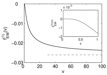
Figure 10: Function $f^{(1)}_{EW}(v)$ (solid) [Eq.(VIII.2)]. The asymptotic limit at large values of $v$ [Eq.(143)] is shown by the dashed line. The inset demonstrates $v^{3}$ behavior at small $v$.

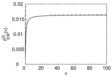
Figure 11: Function $f^{(2)}_{EW}(v)$ (solid) [Eq.(VIII.2)] and its asymptotic limits (dashed) at small and large [Eq.(145)] values of $v$.

Finally, one can establish the correspondence between the function $f(v)$ entering the general formula (118) for the pressure in the limit of one diluted body and the functions $f_{PW}(v)$, $f_{EW}^{(1)}(v)$, and $f_{EW}^{(2)}(v)$ given by Eqs. (131), (VIII.2), and (VIII.2), respectively. This correspondence is given by the simple relation

$$C\;f(v)=f_{PW}(v)+f_{EW}^{(1)}(v)+f_{EW}^{(2)}(v).$$ (149)

IX Large distance behavior of the surface-atom force out of thermal equilibrium

It is interesting to recover the asymptotic results of the surface-atom force out of thermal equilibrium (obtained in articolo2 ) from the general expression of the pressure given by Eqs.(62) and (63). To do this it is crucial to carry out the limit $(\varepsilon_{2}-1)=4\pi n\alpha_{2}\rightarrow 0$ before taking the limit of large distances. To show this, let us focus first on the EW term given by Eq.(63), and perform the rarefied body expansion (body 2) assuming that $\sqrt{\varepsilon_{20}-1}$ is the smallest quantity, also with respect to $|q_{z}|/k$. Due to the effect of the Bose factor, only the frequencies $\omega\sim k_{B}T/\hbar$ are relevant in the integration, and due to the exponential $e^{-2l|q_{z}|}$ the relevant wave-vectors are given by

$$|q_{z}|/k\sim\lambda_{T}/l\gg\sqrt{\varepsilon_{20}-1}.$$ (150)

In this way at large distance it is easy to reproduce the Eqs.(10)-(11) of articolo2 :

$$\!\!\!\!\!\!\!\!\!\!\!{P}_{\text{th}}^{\text{neq,EW}}(T,0,l)=\frac{\hbar\left(\varepsilon_{20}-1\right)}{l^{2}\;8\pi^{2}\;c}\int_{0}^{\infty}\text{d}\omega\frac{\omega}{e^{\hbar\omega/k_{B}T}-1}\;\times$$ (151)

$$\!\!\!\sqrt{|\varepsilon_{1}(\omega)-1|+\left[\varepsilon_{1}^{\prime}(\omega)-1\right]}\;\frac{2+|\varepsilon_{1}(\omega)-1|}{\sqrt{2}|\varepsilon_{1}(\omega)-1|}.$$

In deriving Eq.(151) we also replaced $\varepsilon_{2}\left(\omega\right)$ with its static value $\varepsilon_{20}$, which is reasonable if $k_{B}T$ is much smaller than the lowest atomic resonances, and also ensures that the atoms of the dilute body $2$ cannot adsorb the thermal radiation.

For a rarefied body one has that $\varepsilon_{20}-1\approx 4\pi\alpha_{0}n_{a}$, where $n_{a}$ is the number of atoms of the body per unit volume and $\alpha_{0}$ is the static polarizability of an atom. The pressure in this case is proportional to $n_{a}$ and the force acting on an individual atom can be calculated as

$$F_{{\rm th}}^{{\rm neq,EW}}=\frac{1}{n_{a}}\frac{dP_{{\rm th}}^{{\rm neq,EW}}}{dl}.$$ (152)

It is easy to check that substituting Eq.(151) into (152) one obtains exactly Eq.(10) of articolo2 .

However, there is also the PW contribution. The expansion in the $l$ -dependent part of the PW pressure (62) produces a contribution identical to the EW one, thereby doubling the value of the force (152). This apparent contradiction can be easily solved by the following arguments. The problem approached in the present paper is not equivalent from that approached in Ref. articolo2 . Here we assume that the second slab, being rarefied, is still thick enough to absorb black body radiation from the first slab. On the contrary, the transition to individual atoms (which is the case discussed in Ref. articolo2 ) demands to completely neglect the absorption. Then, to calculate the surface-atom force correctly, one must consider the limit $\varepsilon_{2}^{\prime\prime}\rightarrow 0$ at finite thickness $L$ of the slab 2. On the contrary using the expression (62) means taking the opposite limit procedure, i.e. first $L\rightarrow\infty$ and later $\varepsilon_{2}^{\prime\prime}\rightarrow 0$. The reason why the first limiting procedure is correct in this case, is that if the slab $2$ does not absorb radiation completely, one should also take into account the pressure acting on the remote surface (i.e. the external one), generated by the radiation coming from the left. In absence of absorption it is possible to show that the inclusion of the remote surface in the slab $2$ results in a relatively small value of the PW pressure. Details of calculations are presented in the Appendix B. We only notice here that neglecting of absorption actually requires the condition $\varepsilon_{2}^{\prime\prime}\ll\lambda_{T}^{2}/lL$.

As a consequence, for a finite slab of rarefied gas without absorption the EW contribution (151) provides the total pressure and is equivalent to equations (10)-(11) of articolo2 for the surface-atom force. In particular at temperatures less than the lowest resonance in $\varepsilon_{1}(\omega)$ the pressure (151) (and hence the total pressure) takes the form articolo2

$$P_{\text{th}}^{\text{neq,EW}}(T,0,l)=\frac{(k_{B}T)^{2}}{48\;l^{2}\;c\hbar}\frac{\varepsilon_{10}+1}{\sqrt{\varepsilon_{10}-1}}\;(\varepsilon_{20}-1).$$ (153)

The above result holds at distances (123).

X Conclusions

In this paper we generalized the Casimir-Lifshitz theory for the surface-surface pressure to a situation out of thermal equilibrium, when two bodies are kept at different temperatures in a stationary configuration. In contrast with the equilibrium case, the non-equilibrium force cannot be presented as the sum over imaginary frequencies and one has to work in the real frequency domain. At real frequencies it is natural to separate contributions from propagating and evanescent waves. The delicate interplay between these contributions set the total force.

For bodies made of similar materials the pressure is expressed via the forces at equilibrium. In the general case there is an additional contribution to the pressure, which is antisymmetric in respect to interchange of the materials. The propagating part of the force contains distance independent terms, due to the presence of an energy flux between the bodies in absence of equilibrium.

We presented a detailed analysis of the force, with particular attention for large separations/high temperature behaviors. At equilibrium significant cancellations between PW and EW contributions occur. Such cancellations are less pronounced in the non-equilibrium situation. It is established that at large distances the force between heated ($T$) and cold ($T=0$) bodies behaves similar to the Lifshitz limit, $\sim T/l^{3}$, but with different numerical coefficient. However, this result is true only for dense bodies. If one of them is diluted the behavior of the force can change.

Special attention was devoted to the case when one body is diluted. This is an important situation from which one can recover the interaction between a body and a single atom. Two remarkable results are found for this situation ShortArticle . First, at very large distances, $l\gg\lambda_{T}/\sqrt{\varepsilon_{20}-1}$, the pressure becomes non-additive, in contrast with the equilibrium case. Namely, the non-equilibrium pressure is proportional to the square root of the density of the diluted body, while in the equilibrium it is proportional to the first power of the density and, therefore, it is additive. The second result concerns smaller distances, $\lambda_{T}\ll l\ll\lambda_{T}/\sqrt{\varepsilon_{20}-1}$. In this case we found a new asymptotic behavior for the pressure, $\sim T^{2}/l^{2}$, that decays with the distance more slowly than the Lifshitz limit at equilibrium, and has a stronger temperature dependence. A careful analysis of the transition region between these two limits was done both analytically and numerically.

The pressure between diluted and dense bodies in the distance range $\lambda_{T}\ll l\ll\lambda_{T}/\sqrt{\varepsilon_{20}-1}$ is used to deduce the surface-atom force. Earlier and with different methods it was found in articolo2 that at large distances this force must behave as $\sim T^{2}/l^{2}$. The direct transition from the case of the surface-diluted body provides a force which is two times larger than that in Ref. articolo2 , and both EW and PW terms contribute in the same way. We provided a detailed explanation why if the atom does not absorb radiation one has to neglect the contribution of the PW term, hence recovering the known result.

XI Acknowledgments

We acknowledge supports by the INFN-MICRA project and the Ministero dell’Istruzione, dell’ Universitá e della Ricerca (MiUR).

Appendix A Green functions for two parallel dielectric half-spaces

In this section we present the Green function, which is a solution of Eq.(7). We use the Sipe Green-function formalism Sipe for surface optics. Sipe formulated the problem in terms of $s-$ and $p-$polarized EM vectors waves, in of the Fresnel coefficients of the interfaces. Here we use the lateral Fourier transform representation for the Green’s function:

$$G_{ij}\left[\omega;{\bf r},{\bf r}^{\prime}\right]=\int\frac{\textrm{d}^{2}{\bf Q}}{(2\pi)^{2}}\;e^{i{\bf Q}\cdot({\bf R}-{\bf R}^{\prime})}\;g_{ij}\left[\omega;{\bf Q},z,z^{\prime}\right].$$ (154)

In our geometry the Fourier transform $g_{ij}\left[\omega;{\bf Q},z,z^{\prime}\right]$ depends only from the modulus $Q=|{\bf Q}|$.

A.1 Green’s function with the source and the observation points in the vacuum gap

If both the observation point ${\bf r}$ and the source point ${\bf r}^{\prime}$ are in the vacuum gap, the Green function can be written as the sum $G_{ij}\left[\omega;{\bf r},{\bf r}^{\prime}\right]=G_{ij}^{\textrm{sc.}}\left[\omega;{\bf r},{\bf r}^{\prime}\right]+G_{ij}^{\textrm{bu.}}\left[\omega;{\bf r},{\bf r}^{\prime}\right]$, of a scattered and bulk part. In particular the Fourier transform of these terms are Tomas95 :

$$g_{ij}^{\textrm{sc.}}\left[\omega;{\bf Q},z,z^{\prime}\right] = \frac{2\pi ik^{2}}{q_{z}}\sum_{\mu=s,p}\frac{1}{D_{\mu}}\left[{e}_{\mu,i}(+)\;{e}_{\mu,j}(+)\;r_{1}^{\mu}r_{2}^{\mu}\;e^{iq_{z}(z-z^{\prime}+2l)}+{e}_{\mu,i}(+)\;{e}_{\mu,j}(-)\;r_{1}^{\mu}\;e^{iq_{z}(z+z^{\prime})}+\right.$$ (155)

$$\left.{e}_{\mu,i}(-)\;{e}_{\mu,j}(+)\;r_{2}^{\mu}\;e^{-iq_{z}(z+z^{\prime}-2l)}+\right.\left.{e}_{\mu,i}(-)\;{e}_{\mu,j}(-)\;r_{1}^{\mu}r_{2}^{\mu}\;e^{-iq_{z}(z-z^{\prime}-2l)}\right],$$

$$g_{ij}^{\textrm{bu.}}\left[\omega;{\bf Q},z,z^{\prime}\right] = -4\pi\delta_{i3}\delta_{j3}\delta(z-z^{\prime})+$$ (156)

$$\frac{2\pi ik^{2}}{q_{z}}\sum_{\mu=s,p}\left[{e}_{\mu,i}(+)\;{e}_{\mu,j}(+)\;e^{iq_{z}(z-z^{\prime})}\;\theta(z-z^{\prime})+{e}_{\mu,i}(-)\;{e}_{\mu,j}(-)\;e^{-iq_{z}(z-z^{\prime})}\;\theta(z^{\prime}-z)\right].$$

Here the multiple reflections enter only in the scattered term and are described by the denominator

$$D_{\mu}=1-r^{\mu}_{1}r^{\mu}_{2}e^{2iq_{z}l}.$$ (157)

A.2 Green’s function with the source in a body and the observation point in the vacuum gap

The Fourier transform of the transmitted Green functions with the observation point ${\bf r}$ in the vacuum gap and the source point ${\bf r}^{\prime}$ in the body $1$ or $2$, are respectively Tomas95 :

$$g_{ij}^{(1)}\left[\omega;{\bf Q},z,z^{\prime}\right] = \frac{2\pi ik^{2}}{q_{z}^{(1)}}\sum_{\mu=s,p}\frac{t^{\mu}_{1}}{D_{\mu}}\left[{e}_{\mu,i}(+)\;{e}_{\mu,j}^{(1)}(+)\;e^{iq_{z}z}+{e}_{\mu,i}(-)\;{e}_{\mu,j}^{(1)}(+)\;r_{2}^{\mu}\;e^{-iq_{z}z}\;e^{2iq_{z}l}\right]\;e^{-iq_{z}^{(1)}z^{\prime}},$$ (158)

$$g_{ij}^{(2)}\left[\omega;{\bf Q},z,z^{\prime}\right] = \frac{2\pi ik^{2}}{q_{z}^{(2)}}\sum_{\mu=s,p}\frac{t^{\mu}_{2}}{D_{\mu}}\left[{e}_{\mu,i}(-)\;{e}_{\mu,j}^{(2)}(-)\;e^{-iq_{z}z}+{e}_{\mu,i}(+)\;{e}_{\mu,j}^{(2)}(-)\;r_{1}^{\mu}\;e^{iq_{z}z}\right]\;e^{iq_{z}l}\;e^{iq_{z}^{(2)}(z^{\prime}-l)}.$$ (159)

The symmetry of the problem becomes clear when one set the origin of the coordinate axis in the center of the vacuum gap, by changing $z\rightarrow z-l/2$ and $z^{\prime}\rightarrow z^{\prime}-l/2$ in Eq.(155), (158) and (159).

Appendix B Force acting on a rarefied slab

As discussed in Sec. IX, in order to recover the surface-atom force starting from the surface-surface expression, one must consider the rarefied body as occupying a slab of finite thickness. In this case, for non absorbing atom the PW term of the pressure is negligible, and the EW one reproduces entirely the surface-atom force derived in articolo2 . In this section we discuss this problem and show explicitly that the PW term can be neglected. Let us consider the problem of the thermal forces between a body $1$ at temperature $T$, which occupies the half-space ($z<0$), and a body $2$ at zero temperature which occupies a slab of thickness $L$ in the region ($l<z<l+L$). In the gap $0<z<l$ (region $0$) and outside of the slab $z>l+L$ (region $3$) we can take $\varepsilon=1$. The force per unit of area, acting on the slab in $z-$direction, is

$$P\left(T,0\right)=P^{(0)}-P^{(3)}=\left\langle T_{zz}^{\left(0\right)}\right\rangle-\left\langle T_{zz}^{\left(3\right)}\right\rangle,$$ (160)

where $T_{zz}^{\left(0\right)}$ and $T_{zz}^{\left(3\right)}$ are the $zz-$component of the Maxwell stress tensor in vacuum, calculated in the regions $0$ and $3$, respectively. For a completely absorbing slab there is no field in the region $3$, $T_{zz}^{\left(3\right)}=0$ and one return to Eq.(1). Of course from (160) one can calculate the force acting on a slab of arbitrary thickness, and can recover the results of this paper relative to a thick slab. Here we we assume that the slab is rarefied:

$$\varepsilon_{20}-1\ll 1\ .$$ (161)

Our goal will be to prove that for a slab without absorption the propagating waves give the contribution $P^{{\rm PW}}\ll P^{{\rm EW}}$, and hence can be neglected. For the proof it is enough to consider a monochromatic component of the thermal radiation impinging on the surface of the body 2 with the wave vector ${\bf k}$ and polarization $\mu=s,p.$ In the terms of the complex amplitudes of the fields its contribution to the pressure can be written as [we omit $\left(\mu,{\bf k}\right)$ arguments of the fields]

$$T_{zz}\left(\mu,{\bf k}\right)=\frac{1}{8\pi}\left(\left|E_{z}\right|^{2}-\frac{1}{2}\left|{\bf E}\right|^{2}+\left|H_{z}\right|^{2}-\frac{1}{2}\left|{\bf H}\right|^{2}\right).$$ (162)

The fields in the region 0 are the sums of incident $\left(+\right)$ and reflected $\left(-\right)$ waves:

$${\bf E}^{\left(0\right)}={\bf E}^{\left(0+\right)}+{\bf E}^{\left(0-\right)},\;\;\;\;\;{\bf H}^{\left(0\right)}={\bf H}^{\left(0+\right)}+{\bf H}^{\left(0-\right)}{\rm\ ,}$$ (163)

where ${\bf E}^{\left(0+\right)},{\bf H}^{\left(0+\right)}\propto e^{iq_{z}z}$ and ${\bf E}^{\left(0-\right)},{\bf H}^{\left(0-\right)}\propto e^{-iq_{z}z}$. An important point of the proof is that incident and reflected waves give independent contributions to the stress tensor:

$$T_{zz}^{\left(0\right)}=T_{zz}^{\left(0+\right)}+T_{zz}^{\left(0-\right)}.$$ (164)

The additivity property (164) is obvious. Presence of the mixed term containing both ${\bf E}^{\left(0+\right)}$ and ${\bf E}^{\left(0-\right)\ast}$ would result in the $z-$dependence of $T_{zz}$. But this is not possible since it violates the momentum conservation.
By definition we have that

$$\left|{\bf E}^{\left(0-\right)}\left(\mu,{\bf k}\right)\right|^{2}=R^{\left(\mu,{\bf k}\right)}\left|{\bf E}^{\left(0+\right)}\left(\mu,{\bf k}\right)\right|^{2},$$ (165)

where $R^{\left(\mu,{\bf k}\right)}$ is the reflection coefficient from the slab, for the $(\mu,{\bf k})$-wave . Taking into account the Fresnel relations between the field components at the reflection, we easily find that

$$T_{zz}^{\left(0-\right)}=RT_{zz}^{\left(0+\right)},\;\;\;\;\;\;\;\;T_{zz}^{\left(0\right)}=\left(1+R\right)T_{zz}^{\left(0+\right)}.$$ (166)

Let us consider now the fields in the vacuum region 3. There is only a refracted wave and we have $\left|{\bf E}^{\left(3\right)}\right|^{2}=D^{\left(\mu,{\bf k}\right)}\left|{\bf E}^{\left(0+\right)}\right|^{2}$, where  $D^{\left(\mu,{\bf k}\right)}$ is the transmission coefficient. In absence of absorption $D^{\left(\mu,{\bf k}\right)}=1-R^{\left(\mu,{\bf k}\right)}$. This means that

$$T_{zz}^{\left(3\right)}\left(\mu,{\bf k}\right) = \left(1-R^{\left(\mu,{\bf k}\right)}\right)T_{zz}^{\left(0+\right)}\left(\mu,{\bf k}\right)$$ (167)

$$= \frac{1-R^{\left(\mu,{\bf k}\right)}}{1+R^{\left(\mu,{\bf k}\right)}}T_{zz}^{\left(0\right)}\left(\mu,{\bf k}\right),$$

and from (160) one has

$$P^{{\rm PW}}\left(\mu,{\bf k}\right)=\frac{2R^{\left(\mu,{\bf k}\right)}}{1+R^{\left(\mu,{\bf k}\right)}}T_{zz}^{\left(0\right)}\ \left(\mu,{\bf k}\right).$$ (168)

One can easily calculate $R^{\left(\mu,{\bf k}\right)}$, (see, for example, the problem N.4 in § 66 of LLPCM ). At real $\varepsilon_{20}\rightarrow 1$ one gets, independently on the polarization, the result:

$$R^{\left(\mu,{\bf k}\right)}\approx\frac{\sin^{2}\left[\frac{\omega L}{c}\cos\theta_{0}\right]}{4\cos^{4}\theta_{0}}\left(\varepsilon_{20}-1\right)^{2},$$ (169)

where $\theta_{0}$ is the angle of incidence. This equation is valid at the condition $\cos\theta_{0}\gg\sqrt{\varepsilon_{20}-1}\ .$ Let us note that the surface-atom force equations of articolo2 must be valid in the ”additive“ regime of the Sec. VIII, where just the incident angles $\cos\theta_{0}=q_{z}/k\sim\lambda_{T}/l$ $\gg\sqrt{\varepsilon_{20}-1}$  are important [see Eq.(150)]. For such angles $R^{\left(\mu,{\bf k}\right)}\sim\left(l\sqrt{\varepsilon_{20}-1}/\lambda_{T}\right)^{4}\ll 1$, and $P^{{\rm PW}}\ll T_{zz}^{\left(0\right)}$. Here we assumed that $l$ $\gg\lambda_{T}$.  For $l$ $\lesssim\lambda_{T}$ one gets simply $R^{\left(\mu,{\bf k}\right)}\sim\left(\varepsilon_{20}-1\right)^{2}$. It is not difficult to check that $T_{zz}^{\left(0\right)}\sim$ $\left(\varepsilon_{20}-1\right)\sim P^{{\rm EW}}.$ Finally we find that $P^{{\rm PW}}\ll P^{{\rm EW}}$ and hence the propagating waves contribution can be neglected.

Let us discuss now the role of a weak absorption. Consider the case

$$\varepsilon_{2}=\varepsilon_{2}^{\prime}+i\varepsilon_{2}^{\prime\prime},\varepsilon_{2}^{\prime\prime}\ll 1,\varepsilon_{2}^{\prime}\approx 1.$$ (170)

It is not difficult to generalize (168) for a slab with absorption:

$$P^{{\rm PW}}=\left(1-\frac{D}{1+R}\right)T_{zz}^{\left(0\right)},$$ (171)

where the transmission coefficient $D<1-R$. If $R\ll 1,$

$$P^{{\rm PW}}\approx\left(1-D\right)T_{zz}^{\left(0\right)}.$$ (172)

According to Problem 4 of § 66 in LLPCM , one has that $D\sim\exp\left(-\frac{\omega L\varepsilon_{2}^{\prime\prime}}{c\cos\theta_{0}}\right).$ The imaginary part  $\varepsilon_{2}^{\prime\prime}\left(\omega\right)$ must be taken in this estimate at $\omega\sim k_{B}T/\hbar.$ The factor $\left(1-D\right)$ and correspondingly $P^{{\rm PW}}$ are small if $\omega L\varepsilon_{2}^{\prime\prime}\ll c\cos\theta_{0}$. This gives the condition for neglecting the absorption:

$$\varepsilon_{2}^{\prime\prime}\left(\omega\sim k_{B}T/\hbar\right)\ll\lambda_{T}^{2}/lL.$$ (173)

Let us note that for evanescent waves $T_{zz}^{\left(3\right){\rm EW}}$ does not depend on $z$, while the field of an evanescent wave goes to zero at $z\rightarrow\infty$. This means that $T_{zz}^{\left(3\right){\rm EW}}\equiv 0$.

References

- (1) H.B.G. Casimir, Proc. K. Ned. Akad. Wet. 51, 793 (1948).
- (2) H.B.G. Casimir and D. Polder, Phys. Rev. 73, 360 (1948).
- (3) E.M. Lifshitz, Dokl. Akad. Nauk SSSR 100, 879 (1955).
- (4) E. M. Lifshitz, Zh. Eksp. Teor. Fiz. 29, 94 (1956) [Sov. Phys. JETP 2, 73 (1956)].
- (5) E.M. Lifshitz, Sov. Phys. JETP, 3, 977 (1957).
- (6) S.M. Rytov, Y.A. Kravtsov and V.I. Tatarskii, Principles of Statistical Radiophysics, vol.3: Elements of Random Fields (Springer, Berlin, 1989). This is an enlarged edition of: S.M. Rytov, Theory of Electric Fluctuations and Thermal Radiation (Academy of Sciences of USSR, Moscow, 1953, in Russian).
- (7) I.E. Dzyaloshinskii, E.M. Lifshitz and L.P. Pitaevskii, Advances in Physics 10, 165 (1961).
- (8) C. I. Sukenik, M. G. Boshier, D. Cho, V. Sandoghdar, and E. A. Hinds, Phys. Rev. Lett. 70, 560 (1993).
- (9) S. K. Lamoreaux, Phys. Rev. Lett. 78, 5 (1997).
- (10) B.W. Harris, F. Chen, and U. Mohideen, Phys. Rev. A62,052109 (2000).
- (11) H.B. Chan, V.A. Aksyuk, R.N. Kleiman, D.J. Bishop, and F. Capasso, Science 291, 1941 (2001).
- (12) R.S. Decca, D. López, E. Fischbach, and D.E. Krause, Phys. Rev. Lett. 91, 050402 (2003).
- (13) G. Bressi, G. Carugno, R. Onofrio, and G. Ruoso, Phys. Rev. Lett. 88, 041804 (2002).
- (14) M. Antezza, L.P. Pitaevskii, and S. Stringari, Phys. Rev. A70, 053619 (2004).
- (15) D.M. Harber, J.M. Obrecht, J.M. McGuirk, and E.A. Cornell, Phys. Rev. A72, 033610 (2005).
- (16) J.M. Obrecht, R.J. Wild, M. Antezza, L.P. Pitaevskii, S. Stringari, and E.A. Cornell, Phys. Rev. Lett. 98, 063201 (2007).
- (17) M. Antezza, L.P. Pitaevskii, and S. Stringari, Phys. Rev. Lett. 95, 113202 (2005).
- (18) It is useful to mention here some new experiments proposed in order to measure the thermal effects at thermal equilibrium: I. Carusotto, L.P. Pitaevskii, S. Stringari, G. Modugno, M. Inguscio, Phys. Rev. Lett. 95, 093202 (2005) (surface-atom); M. Brown-Hayes, D.A.R. Dalvit, F.D. Mazzitelli, W.J. Kim, and R. Onofrio, Phys. Rev. A72, 052102 (2005) (cylinder-surface); P. Antonini, G. Bressi, G. Carugno, G. Galeazzi, G. Messineo, and G. Ruoso, New J. Phys. 8, 239 (2006) (surface-surface).
- (19) J.P. Rosenkrans, B. Linder, R.A. Kromhout, J. Chem. Phys. 49, 2927 (1968).
- (20) C. Henkel, K. Joulain, J.-P. Mulet, and J.-J. Greffet, J. Opt. A: Pure Appl. Opt. 4, S109 (2002).
- (21) M. Antezza, J. Phys. A: Math. Gen. 39, 6117 (2006).
- (22) L.P. Pitaevskii, J. Phys. A: Math. Gen. 39, 6665 (2006).
- (23) M. Antezza, L.P. Pitaevskii, S. Stringari, and V.B. Svetovoy, Phys. Rev. Lett. 97, 223203 (2006).
- (24) M. Antezza, Thermal dependence of the Casimir-Polder-Lifshitz force and its effect on ultra-cold gases, (Ph.D. Thesis, University of Trento, Italy, 2006).
- (25) I.A. Dorofeyev, J. Phys. A: Math. Gen. 31, 4369 (1998).
- (26) I. Dorofeyev, H. Fuchs, and J. Jersch, Phys. Rev. E 65, 026610 (2002).
- (27) K. Joulain, J.-P. Mulet, F. Marquier, R. Carminati, J.-J. Greffet, Surf. Sci. Rep. 57, 59 (2005).
- (28) D. Polder and M. Van Hove, Phys. Rev. B 4, 3303 (1971).
- (29) G. Bimonte, Phys. Rev. Lett. 96, 160401 (2006).
- (30) L.D. Landau and E.M. Lifshitz, Electrodynamics of Continuos Media, (Pergamon Press, Oxford, 1963).
- (31) If and are the pressures acting respectively on the bodies and , we have that . Then a positive sign for corresponds to an attraction between the two plates, while a negative sign corresponds to a repulsion.
- (32) E.M. Lifshitz and L.P. Pitaevskii, Statistical Physics, Part 2, (Pergamon Press, Oxford, 1991).
- (33) G.S. Agarwal, Phys. Rev. A11, 230 (1975).
- (34) R. Matloob, H. Falinejad, Phys. Rev. A64, 042102 (2001).
- (35) The condition requiring the divergences of as selects the advanced Green’s function LP ; AGD .
- (36) A.A. Abrikosov, L.P. Gorkov, and I.E. Dzyaloshinski, Methods of Quantum Fields Theory in Statistical Physics, (Prentice-Hall, Englewood Cliffs, USA, 1963).
- (37) J.M. Wylie and J.E. Sipe, Phys. Rev. A30, 1185 (1984); J.E. Sipe, J. Opt. Soc. Am. B 4, 481 (1987).
- (38) M. Revzen, R. Opher, M. Opher, A. Mann, J. Phys. A: Math. Gen. 30, 7783 (1997).
- (39) M.S. Tomas, Phys. Rev. A51, 2545 (1995).
- (40) M.S. Tomas, Phys. Rev. A66, 052103 (2002).
- (41) W. Eckhardt, Phys. Rev. A29, 1991 (1984).
- (42) C.H. Henry and R.F. Kazarinov, Rev. Mod. Phys. 68, 801 (1996).
- (43) V.B. Svetovoy and R. Esquivel, Phys. Rev. E 72, 036113 (2005).
- (44) M. Boström and B.E. Sernelius, Phys. Rev. Lett. 84, 4757 (2000).
- (45) A strong cancellation between contributions of propagating and evanescent waves at was discovered by F. Intravaia and A. Lambrecht, Phys. Rev. Lett. 94, 110404 (2005) and also F. Intravaia, Casimir Effect and Interaction between Surface Plasmons (2006), (Ph.D. Thesis, Université Pierre et Marie Curie - Paris VI, on-line at http://tel.archives-ouvertes.fr/tel-00009755).
- (46) C. Henkel, private communication.
- (47) W.J. Tropf and M.E. Thomas, in Handbook of optical constants of solids, edited by E. Palik (Academic Press, New York, 1998), Vol. III.
- (48) Handbook of mathematical functions, edited by M. Abramowitz and I. A. Stegun (National Bureau of Standards, Applyed Mathematics Series 55, 1972).