Failure of standard approximations of the exchange coupling in nanostructures

Abstract

We calculate the exchange coupling for a double dot system using a numerically exact technique based on finite-element methods and an expansion in 2D Gaussians. Specifically, we evaluate the exchange coupling both for a quasi-one and a two-dimensional system, also including an applied magnetic field. Our numerical results provide a stringent test of standard approximation schemes (e.g., Heitler–London, Hund–Mulliken, Hubbard), and they show that the standard methods do not have reliable predictive power even for simple model systems. Their value in modeling more realistic quantum-dot structures is thus cast in serious doubt.

I Introduction

The possibility of coherent manipulation of electron spins in low-dimensional nanostructures, aimed at future large-scale quantum information processing,Loss and DiVincenzo (1998) calls for a thorough understanding of the spin interactions at play. In the proposal for quantum computing with quantum dots by Loss and DiVincenzo, the exchange coupling between the spins of electrons in tunnel-coupled quantum dots was envisioned as the controllable mechanism for coherent manipulation of spin qubits.Loss and DiVincenzo (1998); Burkard et al. (1999) Recently, this fundamental building block of a possible future solid-state quantum computing architecture was realized in an experiment, demonstrating electrostatic control of the exchange coupling.Petta et al. (2005)

In this paper we present numerically exact finite-element methods for calculations of the exchange coupling between electron spins in tunnel-coupled quasi-one and two-dimensional quantum dots. Such structures have already been under intensive theoretical investigation using various numerical methods, e.g. based on an exact diagonalization of the underlying Hamiltonian Szafran et al. (2004); Bellucci et al. (2004); Helle et al. (2005); Zhang et al. (2006); Melnikov and Leburton (2006); Melnikov et al. (2006); Zhang et al. (2007) or using quantum-chemical approaches like self-consistent Hartree–Fock methods.Hu and Das Sarma (2000) Such numerical approaches often require extensive numerical work. Therefore, much attention has been devoted to simple approximations which lead to closed-form analytic expressions for the exchange coupling.Burkard et al. (1999); Calderon et al. (2006); Saraiva et al. (2007) It is, however, not immediately obvious to what extent these approximations yield correct predictions, and where they break down. For example, in a recent workCalderon et al. (2006) the validity criterion for such approximations was the requirement that the exchange coupling at zero magnetic field always must be positive. A criterion like this can only provide a necessary condition for an approximate scheme to be acceptable.

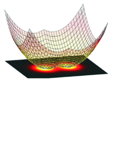
Figure 1: (Color online). Double quantum dot and numerically calculated charge density. The double quantum dot is described by the potential $V(\mathbf{r})$ given in Eq. (4) (here with $\alpha=1$, $\hbar\omega_{0}=4$ meV and $d/r_{0}=1$). The two-dimensional contour plot shows how the charge of two electrons in a singlet spin state is distributed within the double quantum dot. With finite tunnel-coupling between the two quantum dots, the spins of the electrons interact due to the exchange interaction.

The aim of this work is to provide a quantitative comparison of the Heitler–London, the Hund–Mulliken, and the Hubbard approximations, applied to a simple model potential of a double quantum dot, with numerically exact results. In particular, we focus on the case, where the distance between the two quantum dots is short, such that the single-dot electron wave functions have a large overlap. For short distances, the exchange coupling can reach values on the order of several meV, making it sufficiently large to exploit and observe in experiments, and our comparative study is thus highly relevant for on-going experimental activities within the field. The finite-element methods used here allow an easy implementation using available numerical packages,www.comsol.com also when finite magnetic fields are included, which strongly influence the exchange coupling in two-dimensional geometries. We find that the approximative schemes may provide reasonable predictions of the exchange coupling for certain parameter ranges, while they fail, also qualitatively, for short distances, even for the simple model potential considered here. Their value in modeling more realistic quantum-dot structures used in experiments is thereby cast in serious doubt.

II Double quantum dot model

Experimentally, electrons can be confined in double quantum dots using metallic gates on top of a semiconductor heterostructurePetta et al. (2005); Koppens et al. (2005); Hatano et al. (2005) or across a nanowireFasth et al. (2005); Shorubalko et al. (2007) or a nanotube.Sapmaz et al. (2006); Jœrgensen et al. (2006) By suitable electrostatic gating such Coulomb-blockade double quantum dots can be brought into a few-electron regime,van der Wiel et al. (2003) where only a single electron occupies each of the two quantum dots. In this regime, the spin and charge dynamics are described by a two-electron Hamiltonian of the form

$$H(\mathbf{r}_{1},\mathbf{r}_{2})=h(\mathbf{r}_{1})+h(\mathbf{r}_{2})+C(|\mathbf{r}_{1}-\mathbf{r}_{2}|),$$ (1)

where

$$C(|\mathbf{r}_{1}-\mathbf{r}_{2}|)=\frac{e^{2}}{4\pi\varepsilon_{r}\varepsilon_{0}|\mathbf{r}_{1}-\mathbf{r}_{2}|}$$ (2)

is the Coulomb interaction and the single-particle Hamiltonians are

$$h(\mathbf{r})=\frac{\mathbf{p}^{2}}{2m}+V(\mathbf{r}),$$ (3)

with $V(\mathbf{r})$ denoting the confining potential. As in many realizations of double quantum dots we assume that the motion of the electrons is restricted to maximally two dimensions, i.e., $\mathbf{r}=(x,y)$. The inclusion of a magnetic field is discussed below.

As an illustrative example we consider a simple double dot potential readingHelle et al. (2005); Helle (2006)

$$V(\mathbf{r})=\frac{m\omega_{0}^{2}}{2}\left[\min\{(x-d)^{2},(x+d)^{2}\}+(\alpha y)^{2}\right].$$ (4)

Here, $m$ is the effective electron mass, $\hbar\omega_{0}$ is the characteristic confinement energy, $2d$ measures the center to center distance between the quantum dots, and $\alpha$ denotes the ratio of the confinement strengths in the $x$ and $y$ directions. Moreover, we introduce the characteristic oscillator length $r_{0}=\sqrt{\hbar/m\omega_{0}}$. The potential is shown in Fig. 1 together with a numerically calculated charge density. In the limit $d\rightarrow 0$, the potential reduces to that of a single quantum dot. In our calculations we use material parameters typical of GaAs ($m=0.067m_{e}$, $\varepsilon_{r}=12.9$). We consider both the quasi-one dimensional limit $\alpha\gg 1$ and the two-dimensional case $\alpha=1$.

The exchange coupling between the two electrons is a purely orbital effect which arises as a consequence of the Pauli principle and the Coulomb interaction which lead to a splitting $J=E_{A}-E_{S}$ of the lowest eigenvalue $E_{S}$ corresponding to a symmetric orbital wavefunction of the two electrons, $\Psi_{S}(\mathbf{r}_{1},\mathbf{r}_{2})=\Psi_{S}(\mathbf{r}_{2},\mathbf{r}_{1})$, and the lowest eigenvalue $E_{A}$ corresponding to an anti-symmetric orbital wavefunction, $\Psi_{A}(\mathbf{r}_{1},\mathbf{r}_{2})=-\Psi_{A}(\mathbf{r}_{2},\mathbf{r}_{1})$. Due to the Pauli principle the orbital part of a singlet state must be symmetric, while the orbital part of a triplet state must be anti-symmetric. The splitting of the orbital wavefunctions may thereby be mapped onto an effective spin Hamiltonian, $\mathcal{H}=J\,\mathbf{S}_{1}\!\cdot\!\mathbf{S}_{2}$. Ashcroft and Mermin (1976) The task is to calculate the exchange coupling $J$ as function of various parameters, e.g., the distance between the quantum dots and the applied magnetic field. A magnetic field only affects the exchange coupling significantly in two-dimensional geometries and we consequently concentrate on the inclusion of a magnetic field in the two-dimensional case $\alpha=1$.

III Validity of approximate methods

III.1 Quasi-one dimensional limit

We first consider the quasi-one dimensional limit $\alpha\gg 1$, which may be relevant, e.g., for describing confined electrons in nanowires. In this limit we integrate out the motion in the $y$-direction and consider an effective one-dimensional model reading

$$H=h(x_{1})+h(x_{2})+\widetilde{C}_{\alpha}(|x_{1}-x_{2}|),$$ (5)

where the single-electron Hamiltonian is

$$h(x)=\frac{p_{x}^{2}}{2m}+V(x),$$ (6)

$$V(x)=\frac{m\omega_{0}^{2}}{2}[\min\{(x-d)^{2},(x+d)^{2}\}],$$ (7)

and we have introduced

$$\widetilde{C}_{\alpha}(|x|)=\frac{e^{2}}{4\pi\varepsilon_{r}\varepsilon_{0}}\sqrt{\frac{\alpha}{2\pi r_{0}^{2}}}e^{\alpha x^{2}/4r_{0}^{2}}K_{0}(\alpha x^{2}/4r_{0}^{2})$$ (8)

as the (regularized) Coulomb interaction in one dimension. Here, $K_{0}$ is the zeroth-order modified Bessel function of the second kind. The exchange coupling can now be calculated using finite-elements by mapping the one-dimensional two-particle problem onto an effective two-dimensional single-particle problem: We consider the two-particle wavefunction $\Psi(x_{1},x_{2})$ as describing a single fictitious particle with spatial coordinates $\mathbf{\tilde{r}}=(x_{1},x_{2})$ and momentum $\mathbf{\tilde{p}}=(p_{x_{1}},p_{x_{2}})$. Mathematically, the corresponding single-particle-like Hamiltonian then reads

$$H=\mathbf{\tilde{p}}^{2}/2m+W(\mathbf{\tilde{r}}),$$ (9)

where

$$W(\mathbf{\tilde{r}})=V(x_{1})+V(x_{2})+\widetilde{C}_{\alpha}(|x_{1}-x_{2}|)$$ (10)

is the effective external potential that the fictitious particle experiences.

In this reformulation of the problem, the symmetry of the original two-particle wavefunction enters via the boundary condition along the diagonal $x_{2}=x_{1}$. Symmetric wavefunctions fulfill $\Psi_{S}(x_{1},x_{2})=\Psi_{S}(x_{2},x_{1})$ and consequently $\partial_{x_{1}}\Psi_{S}(x_{1},x_{2})|_{x_{2}=x_{1}}=\partial_{x_{2}}\Psi_{S}(x_{1},x_{2})|_{x_{2}=x_{1}}$ (Neumann condition), while anti-symmetric wavefunctions fulfill $\Psi_{A}(x_{1},x_{2})=-\Psi_{A}(x_{2},x_{1})$ and thus $\Psi_{A}(x_{1},x_{2})|_{x_{2}=x_{1}}=0$ (Dirichlet condition). Since $W(\mathbf{\tilde{r}})$ is a confining potential, eigenfunctions go to zero in the limit $|\mathbf{\tilde{r}}|\rightarrow\infty$. In the numerical calculations we assume that the eigenfunctions are zero outside a certain finite range, and we check that the results converge with respect to an increase of this range. Thus, we only need to solve a one-particle problem on a finite-size two-dimensional domain with well-defined boundary conditions. This class of problems is computationally cheap with available finite-element method packages.www.comsol.com

Before discussing the numerical results we briefly review the standard approximations.Burkard et al. (1999) In the Heitler–London approximation the exchange splitting is calculated as $J_{\mathrm{HL}}=\langle-|H|-\rangle-\langle+|H|+\rangle$ with the Heitler–London wavefunctions $|\pm\rangle=(|L\rangle_{1}|R\rangle_{2}\pm|R\rangle_{1}|L\rangle_{2})/\sqrt{2(1\pm|\langle L|R\rangle|^{2})}$, where $H$ is the full two-particle Hamiltonian, and $|L\rangle$ and $|R\rangle$ are the single-particle Fock–Darwin ground states of a single quantum dot centered at $\mathbf{r}_{L}=(-d,0)$ and $\mathbf{r}_{R}=(d,0)$, respectively. The Heitler–London approximation can be improved by including doubly occupied spin singlet states and diagonalizing the Hamiltonian in the resulting Hilbert space. This is known as the Hund–Mulliken approach and yields the expression $J_{\mathrm{HM}}=V-U_{r}/2+\frac{1}{2}\sqrt{U_{r}^{2}+16t_{r}^{2}}$. Here, $U_{r}$ and $t_{r}$ are the on-site Coulomb interaction and the tunnel coupling, respectively, renormalized by the inter-dot Coulomb interaction as described in Ref. Burkard et al., 1999, while $V$ (not to be confused with the confinement potential) is the difference in Coulomb energy between the singly occupied singlet and triplet states. Additional details about the approximative methods are given in Appendix A.

If the inter-dot Coulomb interaction is negligible, the renormalized quantities $U_{r}$ and $t_{r}$ reduce to their bare values, $U$ and $t$, while $V=0$, and if moreover $t/U\ll 1$, the Hund–Mulliken expression reduces to the standard Hubbard expression $J_{\mathrm{H}}=4t^{2}/U$. The Hubbard approximation, which always predicts a positive exchange energy, obviously cannot explain that the exchange energy with an applied magnetic field can be negative. This failure can be corrected by retaining the inter-dot Coulomb interaction, and in the limit $t_{r}/U_{r}\ll 1$, the Hund–Mulliken approximation then yields the extended Hubbard approximation: $J^{*}_{\mathrm{H}}=4t_{r}^{2}/U_{r}+V$. The energy difference $V$ is important for the prediction of the exchange coupling at finite magnetic fields, where it allows for the predicted exchange coupling to become negative.

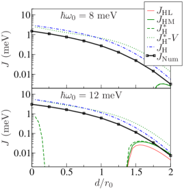
Figure 2: (Color online). Exchange coupling as function of interdot distance in a quasi-one dimensional double quantum dot, $\alpha=10$. The distance $d$ is measured in units of $r_{0}\equiv\sqrt{\hbar/m\omega_{0}}$. Together with the numerical results we show the exchange couplings obtained with the Heitler–London $J_{\mathrm{HL}}$, the Hund–Mulliken $J_{\mathrm{HM}}$, the extended Hubbard $J^{*}_{\mathrm{H}}$, and the standard Hubbard $J_{\mathrm{H}}$ approximations. We also show $J^{*}_{\mathrm{H}}-V$, where $V$ is the Coulomb energy difference between the singly occupied singlet and triplet states.

In Fig. 2 we show numerical results for the exchange coupling as a function of the inter-dot distance with different values of the confinement energy $\hbar\omega_{0}$ for the quasi-one dimensional case $\alpha=10\gg 1$. Together with the numerical results we show the Heitler–London, the Hund–Mulliken and different variations of the Hubbard approximations. The validity of the Heitler–London approximation is strongly dependent on dimensionality due to the increasingly dominating Coulomb interaction in lower-dimensional systems,Calderon et al. (2006) and for the quasi-one dimensional case $J_{\mathrm{HL}}$ is negative in the entire range considered for $\hbar\omega_{0}\leq 8$ meV. The standard Hubbard approximation predicts reasonably well the $d$-dependence, while both the Hund–Mulliken and extended Hubbard approaches lead to (unphysical) negative values of the exchange coupling for a wide range of system parameters. We discuss these discrepancies in more detail when we consider the two-dimensional case below. Confinement energies larger than $18$ meV are required for these approximations to yield positive exchange couplings for all interdot distances. For higher values of $\alpha$, corresponding to stronger confinement in the $y$-direction, the range of validity of these approximations is further reduced.

III.2 Two-dimensional case

We next consider the two-dimensional case $\alpha=1$. In two dimensions the exchange coupling is strongly dependent on applied magnetic fields, and we include a magnetic field perpendicular to the motion of the electrons by the substitution $\mathbf{p}\rightarrow\mathbf{p}+e\mathbf{A}$, where $\mathbf{A}=B_{z}(-y,x)/2$ is a vector potential corresponding to the applied magnetic field $B_{z}\mathbf{\hat{z}}$. The Zeeman term does not affect the exchange coupling and is trivial to include in final total energy calculations.

Rather than mapping the two-dimensional two-particle problem onto an effective four-dimensional one-particle problem, we construct a two-particle basis from single-particle eigenstates $\phi_{i}(\mathbf{r})$ with eigenenergies $\varepsilon_{i}$ found by diagonalizing the single-particle Hamiltonian $h(\mathbf{r})=\frac{(\mathbf{p}+e\mathbf{A})^{2}}{2m}+V(\mathbf{r})$, again using finite-element methods.www.comsol.com The (unsymmmetrized) two-particle basis functions are then $\Psi_{i,j}(\mathbf{r}_{1},\mathbf{r}_{2})=\phi_{i}(\mathbf{r_{1}})\phi_{j}(\mathbf{r_{2}})$, in terms of which the matrix elements of the two-particle Hamiltonian read

$$[\mathbf{H}]_{ij,i^{\prime}j^{\prime}} = \langle\Psi_{i,j}|H|\Psi_{i^{\prime},j^{\prime}}\rangle$$ (11)

$$= (\varepsilon_{i}+\varepsilon_{j})\delta_{i,i^{\prime}}\delta_{j,j^{\prime}}+\langle\Psi_{i,j}|C|\Psi_{i^{\prime},j^{\prime}}\rangle.$$

The Coulomb matrix elements are evaluated by inserting a set of two-particle states constructed from orthonormalized Gaussian single-particle wavefunctions. From the low-energy spectrum of $\mathbf{H}$ we then obtain the exchange coupling $J$. The details of this procedure are described in Appendix B.

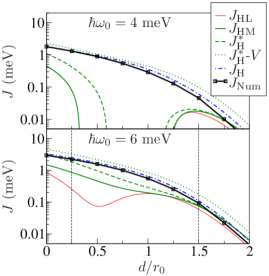
Figure 3: (Color online). Exchange coupling as function of interdot distance in a two-dimensional double dot, $\alpha=1$. See Fig. 2 for details. The vertical lines denote the two values of $d/r_{0}$ for which the dependence on the magnetic field is shown in Fig. 4.

In Fig. 3 we show the results for the two-dimensional case $\alpha=1$. While the standard Hubbard approximation predicts well the $d$-dependence of the exchange coupling, the Heitler–London and the Hund–Mulliken approximations yield predictions that in certain parameter ranges deviate significantly from the numerical results. In particular, in the case $\hbar\omega_{0}=4$ meV a range of distances exists around $d=r_{0}$, where both approximations predict negative exchange couplings. It is well-known that the Heitler–London approximation fails at short distances, when the overlap of the Heitler–London wavefunctions becomes large, and that the range of validity is reduced as the ratio between the Coulomb and confinement energy is increased. Calderon et al. (2006) This explains why the discrepancies are less pronounced in the case $\hbar\omega_{0}=6$ meV. We conjecture that the poor predictions by the Hund–Mulliken and the extended Hubbard approximations are mainly due to the Coulomb energy difference between the singly occupied singlet and triplet states, denoted $V$, overestimating the effects of the inter-dot Coulomb interaction at short distances ($d\sim r_{0}$), leading to a too low (or even negative) exchange energy. For large distances ($d\sim 2r_{0}$), this overestimation decreases and a better agreement with the full numerics is obtained. In the figure we also show $J^{*}_{\mathrm{H}}-V$ which predicts well the exchange coupling, indicating that the effects of the inter-dot Coulomb interaction indeed seem to be overestimated. With larger confinement energies this overestimation becomes less significant, and a better agreement with the numerically exact results is found.

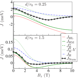
Figure 4: (Color online). Exchange coupling as function of magnetic field in a two-dimensional double dot. Results were obtained with $\hbar\omega_{0}=6$ meV. See Fig. 2 for details.

In Fig. 4 we show numerical results for the exchange coupling as function of the magnetic field $B$ with different inter-dot distances $d$. Together with the numerical results we again show the Heitler–London, the Hund–Mulliken and different variations of the Hubbard approximations. The results show that none of the approximations predict well the dependence of the exchange coupling over the full range of magnetic fields for short distances $d<r_{0}$. For the Hund–Mulliken and the extended Hubbard approximations we again attribute the discrepancy to an overestimation of the effects of the inter-dot Coulomb interaction. For large distances this overestimation is less pronounced, and a good prediction of the qualitative features is obtained.

IV Conclusions

We have presented numerically exact finite-element calculations of the exchange coupling between electron spins confined in low-dimensional nanostructures. We have tested a number of approximations often encountered in the literature by applying them to a simple double dot potential and found that they only predict well the exchange coupling in restricted parameter regimes, when compared to numerical exact results. While the approximative schemes may yield some insight into the qualitative features of the exchange coupling, we find it unlikely that they would suffice in the exchange coupling calculations for actual experimental structures and experiments, having seen how they may fail even in the case of a simple model potential.

We thank A. Braggio, K. Flensberg, L. H. Olsen, A. S. Sørensen, and J. M. Taylor for fruitful discussions. In particular, we thank A. Harju for helpful advice during the development of our numerical routines. APJ is grateful to the FiDiPro program of the Finnish Academy for support during the final stages of this work.

Appendix A Approximative Methods

In the quasi-one dimensional limit $\alpha\gg 1$ we have evaluated the approximative methods numerically using Mathematica, ensuring convergence of the results with respect to a screening length $\delta\rightarrow 0$ of the regularized Coulomb interaction. In the following, we list analytical expressions obtained for the various approximative methods presented in the article for the two-dimensional case $\alpha=1$.

The single-dot potentials corresponding to the double dot potential in Eq. (4) are those of a harmonic oscillator centered at $(\pm d,0)$. The single-dot orbitals are thus the Fock–Darwin states shifted to $(\pm d,0)$. For $d=0$ the Fock–Darwin ground state is

$$\varphi(x,y)=\sqrt{\frac{m\omega}{\pi\hbar}}e^{-m\omega(x^{2}+y^{2})/2\hbar},$$ (12)

where $\omega=\omega_{0}\sqrt{1+\omega_{L}^{2}/\omega_{0}^{2}}$ with $\omega_{L}$ denoting the Larmor frequency $\omega_{L}=eB/2mc$. In the presence of a magnetic field given by the vector potential $\mathbf{A}=B_{z}(-y,x)/2$, shifting the ground state to $(\pm d,0)$ adds a phase factor of $e^{\pm iyd/2l_{B}^{2}}$, where $l_{B}$ is the magnetic length $l_{B}=\sqrt{\hbar c/eB}$. We thus obtain the single-dot orbitals $\varphi_{\pm d}(x,y)=e^{\pm iyd/2l_{B}^{2}}\varphi(x\mp d,y)$, where $\varphi_{\pm d}(x,y)$ then denotes the single-dot orbital centered at $(\pm d,0)$.

Using these single-dot orbitals we obtain for the exchange coupling in the Heitler–London approximation

$$J_{\mathrm{HL}} = \frac{\hbar\omega_{0}}{\mathrm{sinh}\left[2d^{2}(2b-1/b)\right]}\left[c_{s}\frac{\sqrt{\pi b}}{2}\left\{e^{-bd^{2}}I_{0}(bd^{2})\right\}\right.$$

$$+\left.\frac{2d}{\sqrt{b\pi}}\left\{1-e^{-bd^{2}}\right\}+2d^{2}\left\{1-\mathrm{erf}\left(\sqrt{b}d\right)\right\}\right],$$

where $b$ is the magnetic compression factor $b=\omega/\omega_{0}$, $I_{0}$ is the zeroth-order Bessel function, $\mathrm{erf}(x)$ is the error function, and we have introduced the dimensionless distance $d\rightarrow d/r_{0}$. The prefactor $c$ is the ratio between the Coulomb and confining energy, $c_{s}=\frac{e^{2}}{4\pi\epsilon_{r}\epsilon_{0}r_{0}}\frac{1}{\hbar\omega_{0}}$.

In the Hund–Mulliken approximation the exchange coupling is calculated by diagonalizing the two-electron Hamiltonian in the space spanned by $\Psi^{D}_{\pm d}(\mathbf{r}_{1},\mathbf{r}_{2})=\Phi_{\pm d}(\mathbf{r}_{1})\Phi_{\pm d}(\mathbf{r}_{2})$ and $\Psi^{S}_{\pm}(\mathbf{r}_{1},\mathbf{r}_{2})=[\Phi_{+d}(\mathbf{r}_{1})\Phi_{-d}(\mathbf{r}_{2})\pm\Phi_{-d}(\mathbf{r}_{1})\Phi_{+d}(\mathbf{r}_{2})]/\sqrt{2}$, where $\Phi_{\pm d}$ are the orthonormalized single-particle states $\Phi_{\pm d}=(\varphi_{\pm d}-g\varphi_{\mp d})/\sqrt{1-2Sg+g^{2}}$, with $g=(1-\sqrt{1-S^{2}})/S$. This leads to the expression $J_{\mathrm{HM}}=V-U_{r}/2+\frac{1}{2}\sqrt{U_{r}^{2}+16t_{r}^{2}}$, where Burkard et al. (1999)

$$t_{r}=t-w=\left<\Phi_{\pm d}\right|h\left|\Phi_{\mp d}\right>-\left<\Psi_{+}^{S}\right|C\left|\Psi_{\pm d}^{D}\right>/\sqrt{2},$$

$$V=V_{-}-V_{+}=\left<\Psi_{-}^{S}\right|C\left|\Psi_{-}^{S}\right>-\left<\Psi_{+}^{S}\right|C\left|\Psi_{+}^{S}\right>,$$

$$U_{r}=U-V_{+}+X=\left<\Psi_{\pm d}^{D}\right|C\left|\Psi_{\pm d}^{D}\right>-\left<\Psi_{+}^{S}\right|C\left|\Psi_{+}^{S}\right>$$

$$+\left<\Psi_{\pm d}^{D}\right|C\left|\Psi_{\mp d}^{D}\right>.$$ (14)

The Coulomb matrix elements are given by Burkard et al. in Ref. Burkard et al., 1999 and are applicable to any model potential for which the corresponding single-dot potential is a simple harmonic oscillator. Thus only the matrix element $t$ is different for our model potential. We find

$$\frac{t}{\hbar\omega_{0}} = \frac{S}{1-S^{2}}\left[\frac{d}{\sqrt{\pi b}}\left(1-e^{-bd^{2}}\right)+d^{2}\mathrm{erfc}\left(d\sqrt{b}\right)\right],$$

where $\mathrm{erfc}(x)$ is the complimentary error function.

Appendix B Numerical Methods

Here, we discuss the numerical method used in the two-dimensional case $\alpha=1$. We use finite-element methods to solve the single-electron problem given by the single-particle Hamiltonian $h$ in Eq. (1).www.comsol.com The full two-electron problem is then solved by expressing the two-electron Hamiltonian in Eq. (1) in a basis of product states of single-electron solutions $\left|\psi_{n}\right>$, in terms of which the matrix elements are given by Eq. (11). To evaluate the Coulomb elements the single-electron eigenstates are expanded in an orthonormalized basis of 2D Gaussians $\phi_{n_{x},n_{y}}(x,y)=x^{n_{x}}y^{n_{y}}e^{-r^{2}/2}$, where $n_{x}$ and $n_{y}$ are positive integers or zero. The Coulomb matrix elements between product states of 2D Gaussians can be determined analytically, and we state the result here for convenience Pedersen (2007)

$$C_{ijkl} = \frac{e^{2}}{4\pi\epsilon_{0}\epsilon_{r}}\;\frac{\pi}{2}\left(-\frac{1}{4}\right)^{n/2}\sum_{s_{1}=0}^{\lfloor n_{1}/2\rfloor}\cdots\sum_{s_{4}=0}^{\lfloor n_{4}/2\rfloor}\left(-1\right)^{n_{3}+n_{4}+s_{1}+s_{2}-s_{3}-s_{4}}$$

$$\times\;\frac{\Gamma\left(n_{1}+1\right)}{\Gamma\left(s_{1}+1\right)\Gamma\left(n_{1}-2s_{1}+1\right)}\cdots\frac{\Gamma\left(n_{4}+1\right)}{\Gamma\left(s_{4}+1\right)\Gamma\left(n_{4}-2s_{4}+1\right)}$$

$$\times\;\frac{\Gamma\left[\left(n_{1}+n_{3}-2s_{1}-2s_{3}+1\right){/2}\right]\Gamma\left[\left(n_{2}+n_{4}-2s_{2}-2s_{4}+1\right){/2}\right]}{\Gamma\left[\left(n-2s\right){/2}+1\right]}\times\;2^{(n-2s+1)/2}\;\Gamma\left[\left(n-2s+1\right)/2\right],$$

for $n_{1}+n_{3}$ and $n_{2}+n_{4}$ even and zero otherwise. Here $C_{ijkl}=\left<\phi_{n_{x,i},n_{y,i}}\phi_{n_{x,j},n_{y,j}}\right|C\left|\phi_{n_{x,k},n_{y,k}}\phi_{n_{x,l},n_{y,l}}\right>$ while $\Gamma(x)$ is the Gamma function and $\lfloor n/2\rfloor$ indicates flooring of half-integers. Above, we have introduced $n_{1}=n_{x,i}+n_{x,k}$, $n_{2}=n_{y,i}+n_{y,k}$, $n_{3}=n_{x,j}+n_{x,l}$ and $n_{4}=n_{y,j}+n_{y,l}$ , while $n=\sum_{i}n_{i}$ and $s=\sum_{i}s_{i}$. The two-particle Hamiltonian matrix resulting from this procedure may then be diagonalized in the subspaces spanned by the symmetric and antisymmetric product states, respectively, to yield the exchange coupling. Because the expansion in 2D Gaussians becomes increasingly inaccurate as the interdot distance is increased, we are limited to interdot distances of the order of the characteristic oscillator length $r_{0}$. The accuracy of the 2D Gaussian expansion at larger interdot distances could be greatly improved by using an expansion in relative coordinates.Helle et al. (2005)

The finite-element calculations of the single-particle states can be carried out with very high efficiency using existing finite-element packageswww.comsol.com and are not a limiting factor in terms of computational time or convergence. Also, the Coulomb matrix elements $C_{ijkl}$ may be pre-calculated and saved in a lookup table, such that the largest portion of the computational time is spent assembling the two-electron Hamiltonian matrix. For each matrix element, a total of $N^{2}$ lookups in the $C_{ijkl}$ table are required, where $N$ is the number of 2D Gaussians included in the expansion set. A significant reduction in computational time is accomplished by utilizing the symmetry of the Hamiltonian in the product state basis, limiting the calculation to matrix elements which differ by more than a simple complex conjugation. For the results presented in this article, a total of 100 2D Gaussians were used to ensure that the results obtained may essentially be considered exact. With this basis set and a total of $7^{2}=49$ single-particle product states, the calculation of the exchange coupling takes approximately two and a half hours on a standard computer equipped with an Intel Core2 Duo 1.86MHz CPU. As few as 25 Gaussians are in many cases sufficient to produce results that are within 10% of the exact results, and in that case a single calculation only takes about 5 minutes.

The use of finite-element methods for solving the single-electron problem makes it easy to construct the two-electron Hamiltonian, even if analytic expressions for the matrix elements of the single-electron Hamiltonian in the basis of 2D Gaussians cannot easily be obtained. This makes the method very flexible, and only little work is required to solve problems with different choices of potentials. We have verified our numerical implementation against the results in Ref. Helle et al., 2005 as well as for the simple problem of two opposite spin particles in a two-dimensional parabolic potential, which can be solved analytically.

References

- Loss and DiVincenzo (1998) D. Loss and D. P. DiVincenzo, Phys. Rev. A 57, 120 (1998).
- Burkard et al. (1999) G. Burkard, D. Loss, and D. P. DiVincenzo, Phys. Rev. B 59, 2070 (1999).
- Petta et al. (2005) J. R. Petta, A. C. Johnson, J. M. Taylor, E. A. Laird, A. Yacoby, M. D. Lukin, C. M. Marcus, M. P. Hanson, and A. C. Gossard, Science 309, 2180 (2005).
- Szafran et al. (2004) B. Szafran, F. M. Peeters, and S. Bednarek, Phys. Rev. B 70, 205318 (2004).
- Bellucci et al. (2004) D. Bellucci, M. Rontani, F. Troiani, G. Goldoni, and E. Molinari, Phys. Rev. B 69, 201308(R) (2004).
- Helle et al. (2005) M. Helle, A. Harju, and R. M. Nieminen, Phys. Rev. B 72, 205329 (2005).
- Zhang et al. (2006) L. X. Zhang, D. V. Melnikov, and J. P. Leburton, Phys. Rev. B 74, 205306 (2006).
- Melnikov and Leburton (2006) D. V. Melnikov and J. P. Leburton, Phys. Rev. B 73, 155301 (2006).
- Melnikov et al. (2006) D. V. Melnikov, J. P. Leburton, A. Taha, and N. Sobh, Phys. Rev. B 74, 041309(R) (2006).
- Zhang et al. (2007) L. X. Zhang, D. V. Melnikov, and J. P. Leburton, IEEE Trans. Nanotech. 6, 250 (2007).
- Hu and Das Sarma (2000) X. D. Hu and S. Das Sarma, Phys. Rev. A 61, 62301 (2000).
- Calderon et al. (2006) M. J. Calderon, B. Koiller, and S. Das Sarma, Phys. Rev. B 74, 45310 (2006).
- Saraiva et al. (2007) A. L. Saraiva, M. J. Calderon, and B. Koiller, arXiv.org:0706.3354 (2007).
- (14) We have used the COMSOL Multiphysics 3.2 package for all finite-element calculations. See www.comsol.com. Convergence with respect to the mesh size has been ensured.
- Koppens et al. (2005) F. Koppens, J. Folk, J. Elzerman, R. Hanson, L. van Beveren, I. Vink, H. Tranitz, W. Wegscheider, L. Kouwenhoven, and L. Vandersypen, Science 309, 1346 (2005).
- Hatano et al. (2005) T. Hatano, M. Stopa, and S. Tarucha, Science 309, 268 (2005).
- Fasth et al. (2005) C. Fasth, A. Fuhrer, M. T. Björk, and L. Samuelson, Nano Lett. 5, 1487 (2005).
- Shorubalko et al. (2007) I. Shorubalko, A. Pfund, R. Leturcq, M. T. Borgström, F. Gramm, E. Müller, E. Gini, and K. Ensslin, Nanotechnology 18, 44014 (2007).
- Sapmaz et al. (2006) S. Sapmaz, C. Meyer, P. Beliczynski, P. Jarillo-Herrero, and L. P. Kouwenhoven, Nano Lett. 6, 1350 (2006).
- Jœrgensen et al. (2006) H. Jørgensen, K. Grove-Rasmussen, J. Hauptmann, and P. Lindelof, Appl. Phys. Lett. 89, 232113 (2006).
- van der Wiel et al. (2003) W. van der Wiel, S. de Franceschi, J. Elzerman, T. Fujisawa, S. Tarucha, and L. Kouwenhoven, Rev. Mod. Phys. 75, 1 (2003).
- Helle (2006) M. Helle, Ph.D. thesis, Helsinki University of Technology (2006).
- Pedersen (2007) J. Pedersen, Master’s thesis, Technical University of Denmark (2007).
- Leinaas and Myrheim (1977) J. M. Leinaas and J. Myrheim, Nuovo Cimento B 37, 1 (1977).
- Ashcroft and Mermin (1976) N. W. Ashcroft and N. D. Mermin, Solid State Physics (Saunders, Philadelphia, 1976), Chap. 32.