Mathematics University of Leicester

Efficient Method for Detection of Periodic Orbits in Chaotic Maps and Flows

Abstract

An algorithm for detecting unstable periodic orbits in chaotic systems [Phys. Rev. E, 60 (1999), pp. 6172–6175] which combines the set of stabilising transformations proposed by Schmelcher and Diakonos [Phys. Rev. Lett., 78 (1997), pp. 4733–4736] with a modified semi-implicit Euler iterative scheme and seeding with periodic orbits of neighbouring periods, has been shown to be highly efficient when applied to low-dimensional system. The difficulty in applying the algorithm to higher dimensional systems is mainly due to the fact that the number of stabilising transformations grows extremely fast with increasing system dimension. In this thesis, we construct stabilising transformations based on the knowledge of the stability matrices of already detected periodic orbits (used as seeds). The advantage of our approach is in a substantial reduction of the number of transformations, which increases the efficiency of the detection algorithm, especially in the case of high-dimensional systems. The dependence of the number of transformations on the dimensionality of the unstable manifold rather than on system size enables us to apply, for the first time, the method of stabilising transformations to high-dimensional systems. Another important aspect of our treatment of high-dimensional flows is that we do not restrict to a Poincaré surface of section. This is a particularly nice feature, since the correct placement of such a section in a high-dimensional phase space is a challenging problem in itself. The performance of the new approach is illustrated by its application to the four-dimensional kicked double rotor map, a six-dimensional system of three coupled Hénon maps and to the Kuramoto-Sivashinsky system in the weakly turbulent regime.

List of Figures

1. 2.1 (a) The polyhedron ABDC is non-characteristic while the polyhedron AEDC is characteristic, (b) Application of the CB method to AEDC leads to succesive characteristic polyhedra GEDC and HEDC.
2. 2.2 Newton-Raphson method
3. 2.3 After integration time $\tau_{i}$ the point $x_{i}$ returns to the Poincaré surface of section (PSS), however the nearby point $x_{i}+\delta x$ does not. Thus, the matrix needed to map an arbitrary deviation $\delta x_{i}$ on the PSS to the subsequent one $\delta x_{i+1}$ needs to take into account the implicit dependance of the return time on $x$.
4. 3.1 (colour online) Shown in red are the basins of convergence of (a) the Newton method, (b) the Schmelcher and Diakonos method with $0<\lambda<0.3568$ and $C=\mathrm{I}$, and (c) the Davidchack and Lai method with $\beta=4.0$ and $C=\mathrm{I}$ to the zeros of a function $g(x)=\cos(x^{2})$ in the interval $(-3,3)$. Arrows indicate the direction of convergence, and large dots are the zeros to which the method converges.
5. 4.1 Basins of attraction for the period$-3$ orbits of the Ikeda map with parameter values $a=1.0$, $b=0.9$, $k=0.4$ and $\eta=6.0$. Here we have chosen $\tilde{C}=-1$ since in this example the unstable subspace is one-dimensional.
6. 4.2 The basins of attraction for the Ikeda map for the choice of $\tilde{C}=1$. Fixed points of $f^{3}$ with negative unstable eigenvalues are stable stationary solutions of the associated flow, while those with positive eigenvalues are saddles located at the basin boundaries.
7. 4.3 Illustration of two UPOs of KSE detected from a single seed. We show both a level plot for the solutions and a projection onto the first two Fourier components. Since $u(x,t)$ is antisymmetric on $[0,L]$, it is sufficient to display the space-time evolution of $u(x,t)$ on the interval $[0,L/2]$: (a) Seed with time $T=37.0$, (b) a periodic solution of length $T=36.9266$ detected with stabilising transformation $\tilde{C}=+1$ and (c) a periodic solution of length $T=25.8489$ detected with stabilising transformation $\tilde{C}=-1$.
8. 4.4 Illustration of how a UPO can be used as a seed to detect new cycles. We show the projection onto the first two Fourier components of the initial seed ($T=237.4470$) and the three detected orbits. Here $L=38.5$ and $n=15$.
9. 1 The double rotor under the influence of a periodic kick.

List of Tables

1. 3.1 Number $n(p)$ of prime period-$p$ UPOs, and the number $N(p)$ of fixed points of $p$-times iterated map for the kicked double rotor map. The asterisk for $p=8$ indicates that this set of orbits is not complete. Parameters $\epsilon_{\mathrm{max}}(p)$ and $d_{\mathrm{min}}(p)$ are defined in Eqs. (3.34) and (3.35).
2. 3.2 The number of prime UPOs for the system of three coupled Hénon maps (CHM) detected by three different methods: BW – full Biham-Wenzel, BW-r – reduced Biham-Wenzel, ST – our method based on stabilising transformations, Max – maximum number of detected UPOs obtained from all three methods and the system symmetry. See text for details.
3. 4.1 The number of distinct periodic solutions for the Kuramoto-Sivashinsky equation detected by the method of STs. Here $L=38.5$ and $\alpha=0.25$.
4. 4.2 The number of distinct periodic solutions for the Kuramoto-Sivashinsky equation detected by the Levenberg-Marquardt algorithm lmder with $L=38.5$.
5. 4.3 The number of distinct periodic solutions for the Kuramoto-Sivashinsky equation detected by the method of stabilising transformations. Here $L=51.4$ and $\alpha=0.25$.
6. 4.4 The number of distinct periodic solutions for the Kuramoto-Sivashinsky equation detected by the Levenberg-Marquardt algorithm lmder with $L=51.4$.
7. 4.5 Number of distinct orbits detected using the method of stabilising transformations with periodic orbits as seeds The number of seeds is $489$. $L=38.5$, $\alpha=0.25$.
8. 4.6 Number of distinct orbits detected using the method of stabilising transformations with periodic orbits as seeds. The number of seeds is $123$. $L=51.4$, $\alpha=0.25$.

Chapter 1 Introduction

The successes of the differential equation paradigm were impressive and extensive. Many problems, including basic and important ones, led to equations that could be solved. A process of self-selection set in, whereby equations that could not be solved were automatically of less interest than those that could.
I. Stewart

In this chapter we start in §1.1 by giving a brief primer into the theory of dynamical systems. Here our intention is not to give an exhaustive review (concise reviews on the subject are given in [33, 42, 68]). Rather, it is to illustrate the role played by periodic orbits in the development of the theory. In §1.2 a brief introduction to the periodic orbit theory is provided, followed by a discussion concerning the efficient detection of unstable periodic orbits (UPOs). Section 1.3 looks at the application to high-dimensional systems, in particular, large nonequilibrium systems that are extensively chaotic. It is well known that numerical methods can both introduce spurious chaos, as well as suppress it [10, 98]. Thus in §1.4 we discuss some of the numerical issues which can arise when detecting UPOsUPO for a chaotic dynamical system. We give an overview of the objectives of this thesis in §1.5. The final section, 1.6, details the contribution to the literature of this thesis.

1.1 History, theory and applications

Although the subject of modern dynamical systems has seen an explosion of interest in the past thirty years – mainly due to the advent of the digital computer – its roots firmly belong at the foot of the twentieth century. Partly motivated by his work on the famous three body problem, the French mathematician and philosopher Henri Jules Poincaré was to revolutionise the study of nonlinear differential equations.

Since the birth of the calculus, differential equations have been studied both in their own right and for modeling phenomena in the natural sciences. Indeed, Newton considered them in his work on differential calculus [67] as early as $1671$. One of the earliest examples of a first order equation considered by Newton was

$$\frac{dy}{dx}=1-3x+y+x^{2}+xy.$$ (1.1)

A solution of this equation for the initial condition $y(0)=0$ can be obtained as follows: start with

$$y=0+\cdots$$

and insert this into Eq. (1.1); integrating yields

$$y=x+\cdots,$$

repeating the process with the new value of $y$ gives

$$y=x-x^{2}+\cdots.$$

One can imagine continuing this process ad infinitum, leading to the following solution of Eq. (1.1)

$$y=x-x^{2}+\frac{1}{3}x^{3}-\frac{1}{6}x^{4}+\frac{1}{30}x^{5}-\frac{1}{45}x^{6}+\cdots$$

(for further details see [36]).

The preceding example demonstrates one of the main differences between the classical study of differential equations and the current mindset. The classical study of nonlinear equations was local, in the sense that individual solutions where sought after. Most attempts in essence, involved either an approximate series solution or determining a transformation under which the equation was reduced either to a known function or to quadrature.

In his work on celestial mechanics [74], Poincaré developed many of the ideas underpinning modern dynamical systems. By working with sets of initial conditions rather than individual solutions, he was able to prove that complicated orbits existed for which no closed solution was available; Poincaré had caught a glimpse of what is popularly coined “chaos” nowadays.

Although there was continued interest from the mathematical community; most notably Birkhoff in the 1920s and the Soviet mathematicians in the 1940s – Kolmogorov and students thereof – it was not until the 1960s that interest from the general scientific community was rekindled. In 1963 the meteorologist Edward N. Lorenz published his now famous paper “deterministic nonperiodic flow” [61] where a simple system describing cellular convection was shown to exhibit extremely complicated dynamics. Motion was bounded, displayed sensitivity to initial conditions and was aperiodic; Lorenz had witnessed the first example of a chaotic attractor.

Around the same time, the mathematician Steve Smale was using methods from differential topology in order to prove the existence of a large class of dynamical systems (the so called axiom-A systems), which were both chaotic and structurally stable at the same time [91]. Along with examples such as the Lorenz model above, scientists where lead to look beyond equilibrium points and limit cycles in the study of dynamical processes. It became clear that far from being a mathematical oddity, the chaotic evolution displayed by many dynamical systems was of great practical importance.

Today the study of chaotic evolution is widespread throughout the sciences where the tools of nonlinear analysis are used extensively. There remain many open questions and the theory of dynamical systems has a bright and challenging future. The prediction and control [70, 86] of deterministic chaotic systems is an important area which has received a lot of attention over the past decade, whilst the extension of the theory to partial differential equations [79, 93] promises to give fresh insight into the modeling of fully developed turbulence. However, perhaps the most promising area of future research lies in the less mathematically minded disciplines such as biology, economics and the social sciences, to name a few.

1.2 Periodic orbits

Periodic orbits play an important role in the analysis of various types of dynamical systems. In systems with chaotic behaviour, unstable periodic orbits form a “skeleton” for chaotic trajectories [16]. A well regarded definition of chaos [23] requires the existence of an infinite number of UPOs that are dense in the chaotic set. Different geometric and dynamical properties of chaotic sets, such as natural measure, Lyapunov exponents, fractal dimensions, entropies [69], can be determined from the location and stability properties of the embedded UPOs. Periodic orbits are central to the understanding of quantum-mechanical properties of nonseparable systems: the energy level density of such systems can be expressed in a semiclassical approximation as a sum over the UPOs of the corresponding classical system [35]. Topological description of a chaotic attractor also benefits from the knowledge of periodic orbits. For example, a large set of periodic orbits is highly constraining to the symbolic dynamics and can be used to extract the location of a generating partition [20, 73]. The significance of periodic orbits for the experimental study of dynamical systems has been demonstrated in a wide variety of systems [58], especially for the purpose of controlling chaotic dynamics [70] with possible application in communication [5].

1.2.1 Periodic orbit theory

Briefly put, the periodic orbit theory provides a machinery which enables us to use the knowledge provided by the properties of individual solutions, such as their periods, location and stabilities, to make predictions about statistics, e.g. Lyapunov exponents, entropies, and so on. The dynamical systems to be discussed in this section are smooth $n$-dimensional maps of the form $x_{i+1}=f(x_{i})$, where $x_{i}$ is an $n$-dimensional vector in the $n$-dimensional phase space of the system.

Now, in order for the results to be quoted to hold, we assume that the attractor of $f$ is both hyperbolic and mixing. A hyperbolic attractor is one for which the following two conditions hold: (i) there exist stable and unstable manifolds at each point of the attractor whose dimensions, $n_{s}$ and $n_{u}$, are the same for each point on the attractor, with $n_{s}+n_{u}=n$, and (ii) there exists a constant $K>1$ such that for all points, $x$, on the attractor, if a vector $u$ is chosen tangent to the unstable manifold, then

$$||Df(x)u||\geq K||u||,$$ (1.2)

and if $u$ is chosen tangent to the stable manifold

$$||Df(x)u||\leq||u||/K.$$ (1.3)

Here $Df(x)$ denotes the Jacobian matrix of the map $f$ evaluated at the point $x$. By mixing we mean that for any two subsets $A_{1}$, $A_{2}$ in the phase space, we have

$$\lim_{i\to\infty}\mu[A_{1}\cap f^{i}(A_{2})]=\mu(A_{1})\mu(A_{2}),$$ (1.4)

where $\mu$ is the natural measure of the attractor. In other words, the system will evolve over time so that any given open set in phase space will eventually overlap any other given region.

Let us denote the magnitudes of the eigenvalues of the Jacobian matrix for the $p$ times iterated map $f^{p}$ evaluated at the $j$th fixed point by $\lambda_{1j},\dots,\lambda_{nj}$. Suppose that the number of unstable eigenvalues, i.e. $\lambda_{ij}>1$, is given by $n_{u}$, and further, that we order them as follows

$$\lambda_{1j}\geq\cdots\geq\lambda_{n_{u}j}\geq 1\geq\lambda_{(n_{u}+1)j}\geq\cdots\geq\lambda_{nj}.$$ (1.5)

Let $L_{j}$ denote the product of unstable eigenvalues at the $j$th fixed point of $f^{p}$,

$$L_{j}=\lambda_{1j}\lambda_{2j}\cdots\lambda_{n_{u}j}.$$ (1.6)

Then the principal result of the periodic orbit theory is the following: given a subset $A$ of phase space, one may define its natural measure to be

$$\mu(A)=\lim_{p\to\infty}\mu_{p}(A),$$ (1.7)

where

$$\mu_{p}(A)=\sum_{j}L_{j}^{-1}.$$ (1.8)

Here the sum is over all fixed points of $f^{p}$ in $A$; a derivation of Eq. (1.7) may be found in [34].

This result leads to several important consequences, for example, it can be shown that the Lyapunov numbers of $f$ are given by

$$\log\lambda_{p}=\lim_{p\to\infty}\frac{1}{p}\sum_{j}L_{j}^{-1}\log\lambda_{pj},$$ (1.9)

whilst an analogous result exists for the topological entropy

$$h_{T}=\lim_{p\to\infty}\frac{1}{p}\ln N_{p},$$ (1.10)

where $N_{p}$ denotes the number of fixed points of the map $f^{p}$. These and similar results obtained within the periodic orbit theory show that knowledge of the UPOs can yield a great deal of information concerning the properties of a chaotic dynamical system. Thus making their efficient detection highly desirable. For further details, a thorough review of the periodic orbit theory is given in the book by Cvitanović et al [17].

At this stage, it is important to point out that most systems of interest turn out not to be hyperbolic, in particular, the dynamical systems studied in this thesis are non-hyperbolic. Hyperbolic systems, however, remain important due to the fact that they are more tractable from a mathematical perspective. Indeed, most rigorous results in dynamical systems are for the case of hyperbolic systems, and although much of the theory is believed to transfer over to the non-hyperbolic case there are very few rigorous results.

1.2.2 Efficient detection of UPOs

We have seen that the role of UPOs in chaotic systems is of fundamental theoretical and practical importance. It is thus not surprising that much effort has been put into the development of methods for locating periodic solutions in different types of dynamical systems. In a limited number of cases, this can be achieved due to the special structure of the systems. Examples include the Biham-Wenzel method applicable to Hénon-like maps [3], or systems with known and well ordered symbolic dynamics [41]. For generic systems, however, most methods described in the literature use some type of an iterative scheme that, given an initial condition (seed), converges to a periodic orbit of the chaotic system. In order to locate all UPOs with a given period $p$ p, the convergence basin of each orbit for the chosen iterative scheme must contain at least one seed. The seeds are often chosen either at random from within the region of interest, from a regular grid, or from a chaotic trajectory with or without close recurrences. Typically, the iterative scheme is chosen from one of the “globally” convergent methods of quasi-Newton or secant type. However, experience suggests that even the most sophisticated methods of this type suffer from a common problem: with increasing period, the basin size of the UPOs becomes so small that placing a seed within the basin with one of the above listed seeding schemes is practically impossible [64].

A different approach, which appears to effectively deal with the problem of reduced basin sizes has been proposed by Schmelcher and Diakonos (SD) [83, 84] SD. The basic idea is to transform the dynamical system in such a way that the UPOs of the original system become stable and can be located by simply following the evolution of the transformed dynamical system. That is, to locate period-$p$ orbits of a discrete dynamical system U

$$U\!\!:\quad x_{i+1}=f(x_{i}),\quad f\!\!:{\mathbb{R}}^{n}\mapsto{\mathbb{R}}^{n}\;,$$ (1.11)

one considers an associated flow

$$\Sigma\!\!:\quad\frac{dx}{ds}=Cg(x)\,,$$ (1.12)

where $g(x)=f^{p}(x)-x$ and $C$ C is an $n\times n$ n constant orthogonal matrix. It is easy to see that the map $f^{p}(x)$ fg and flow $\Sigma$ sigma have identical sets of fixed points for any $C$, while $C$ can be chosen such that unstable period-$p$ orbits of $U$ become stable fixed points of $\Sigma$.

Since it is not generally possible to choose a single matrix $C$ that would stabilise all UPOs of $U$, the idea is to find the smallest possible set of matrices ${\mathcal{C}}=\{C_{k}\}_{k=1}^{K}$, such that, for each UPO of $U$, there is at least one matrix $C\in{\mathcal{C}}$ that transforms the unstable orbit of $U$ into a stable fixed point of $\Sigma$. To this end, Schmelcher and Diakonos have put forward the following conjecture [83]

Conjecture 1.2.1.

Let ${\mathcal{C}}_{\mathrm{SD}}$ be the set of all $n\times n$ orthogonal matrices with only $\pm 1$ non-zero entries. Then, for any $n\times n$ non-singular real matrix $G$, there exists a matrix $C\in{\mathcal{C}}_{\mathrm{SD}}$ such that all eigenvalues of the product $CG$ have negative real parts.

CSD The set ${\mathcal{C}}_{\mathrm{SD}}$ forms a group isomorphic to the Weyl group $B_{n}$ [48], i.e. the symmetry group of an $n$-dimensional hypercube. The number of matrices in ${\mathcal{C}}_{\mathrm{SD}}$ is $K=2^{n}n!$.

The above conjecture has been verified for $n\leq 2$ [85], and appears to be true for $n>2$, but, thus far, no proof has been presented. According to this conjecture, any periodic orbit, whose stability matrix does not have eigenvalues equal to one, can be transformed into a stable fixed point of $\Sigma$ with $C\in{\mathcal{C}}_{\mathrm{SD}}$. In practice, to locate periodic orbits of the map $U$, we try to integrate the flow $\Sigma$ from a given initial condition (seed) using different matrices from the set ${\mathcal{C}}_{\mathrm{SD}}$. Some of the resulting trajectories will converge to fixed points, while others will fail to do so, either leaving the region of interest or failing to converge within a specified number of steps.

The main advantage of the SD approach is that the convergence basins of the stabilised UPOs appear to be much larger than the basins produced by other iterative schemes [21, 55, 84], making it much easier to select a useful seed. Moreover, depending on the choice of the stabilising transformation, the SD method may converge to several different UPOs from the same seed.

The flow $\Sigma$ can be integrated by any off-the-shelf numerical integrator. Schmelcher and Diakonos have enjoyed considerable success using a simple Euler method. However, the choice of integrator for this problem is governed by considerations very different from those typically used to construct an ODE ODE solver. Indeed, to locate a fixed point of the flow, it may not be very efficient to follow the flow with some prescribed accuracy. Therefore, local error considerations, for example, are not as important. Instead, the goal is to have a solver that can reach the fixed point in as few integration steps as possible. In fact, as shown by Davidchack and Lai [19], the efficiency of the method can be improved dramatically when the solver is constructed specifically with the above goal in mind. In particular, recognizing the typical stiffness of the flow $\Sigma$, Davidchack and Lai have proposed a modified semi-implicit Euler method

$$x_{i+1}=x_{i}+[\beta s_{i}C^{\mathsf{T}}-G_{i}]^{-1}g(x_{i})\;,$$ (1.13)

where $\beta>0$ is a scalar parameter, $s_{i}=||g(x_{i})||$ is an $L_{2}$ norm, $G_{i}=Dg(x_{i})$G is the Jacobian matrix, and “${\mathsf{T}}$” denotes transpose. Note that, away from the root of $g$, the above iterative scheme is a semi-implicit Euler method with step size $h=(\beta s_{i})^{-1}$ and, therefore, can follow the flow $\Sigma$ with a much larger step size than an explicit integrator (e.g. Euler or Runge-Kutta). Close to the root, the proposed scheme can be shown to converge quadratically [55], analogous to the Newton-Raphson method.

Another important ingredient of the algorithm presented in [19] is the seeding with already detected periodic orbits of neighbouring periods. This seeding scheme appears to be superior to the typically employed schemes and enables fast detection of plausibly all periodic orbits of increasingly larger periods in generic low-dimensional chaotic systems. For example, for the Ikeda map at traditional parameter values, the algorithm presented in [19] was able to locate plausibly all periodic orbits up to period 22 for a total of over $10^{6}$ orbit points. Obtaining a comparable result with generally employed techniques requires an estimated $10^{5}$ larger computational effort.

While the stabilisation approach is straightforward for relatively low-dimensional systems, direct application to higher-dimensional systems is much less efficient due to the rapid growth of the number of matrices in ${\mathcal{C}}_{\mathrm{SD}}$. Even though it appears that, in practice, far fewer transformations are required to stabilise all periodic orbits of a given chaotic system [72], the sufficient subset of transformations is not known a priori. It is also clear that the route of constructing a universal set of transformations is unlikely to yield substantial reduction in the number of such transformations. Therefore, a more promising way of using stabilising transformations for locating periodic orbits in high-dimensional systems is to design such transformations based on the information about the properties of the system under investigation.

1.3 Extended systems

The periodic orbit theory is well developed for low-dimensional chaotic dynamics - at least for axiom-A systems [17]. The question naturally arises as to whether or not the theory has anything to say for extended systems. At first glance the transition from low-dimensional chaotic dynamics to fully developed spatiotemporal chaos may seem rather optimistic. However, recent results have shown that certain classes of PDEs PDE turn out to be less complicated than they initially appear, when approached from a dynamical systems perspective. Indeed, under certain conditions their asymptotic evolution can be shown to lie on a finite dimensional global attractor [78, 79, 93]. Further, by restricting to equations of the form

$$\frac{du}{dt}+\mathrm{A}u+F(u)=0,$$ (1.14)

where $A$ is a linear differential operator, an even stronger result may be obtained. Such equations are termed evolution equations and their asymptotic dynamics can be shown to lie on a smooth, finite dimensional manifold, known as the inertial manifold [78]. In contrast to the aforementioned global attractor which may have fractal like properties this leads to a complete description of the dynamics by a finite number of modes; higher modes being contained in the geometrical constraints which define the manifold.

A variety of methods for determining all UPOs up to a given length exist for low-dimensional dynamical systems (see Chapter 2). For more complex dynamics, such as models of turbulence in fluids, chemical reactions, or morphogenesis in biology with high – possibly infinite – dimensional phase spaces, such methods quickly run into difficulties. The most computationally demanding calculation to date, has been performed by Kawahara and Kida [52]. They have reported the detection of two three-dimensional periodic solutions of turbulent plane Couette flow using a $15,422$-dimensional discretisation, whilst more recently Viswanath [95] has been able to detect both periodic and relative periodic motions in the same system. It is hoped that such solutions may act as a basis to infer the manner in which transitions to turbulence can occur.

Our goal is somewhat more modest. We will apply our method to the model example of an extended system which exhibits spatiotemporal chaos; the Kuramoto-Sivashinsky equation

$$u_{t}=-\frac{1}{2}(u^{2})_{x}-u_{xx}-u_{xxxx},\quad t\geq 0,\quad x\in[0,L].$$ (1.15)

It was first studied in the context of reaction-diffusion equations by Kuramoto and Tsuzuki [56], whilst Sivashinsky derived it independently as a model for thermal instabilities in laminar flame fronts [90]. It is one of the simplest PDEs to exhibit chaos and has played a leading role in studies on the connection between ODEs and PDEs [27, 49, 54].

It is the archetypal equation for testing a numerical method for computing periodic solutions in extended systems, and has been considered in this context in [9, 57, 100], where many UPOs have been detected and several dynamical averages computed using the periodic orbit theory. Note that the attractor of the system studied in [9] is low dimensional, whilst those studied in [57, 100] have higher intrinsic dimension. Recently the closely related complex Ginzburg-Landau equation

$$A_{t}=RA+(1+i\nu)A_{xx}-(1+i\mu)A|A|^{2},$$ (1.16)

has been studied within a similar framework [60], where Eq. (1.16) is transformed into a set of algebraic equations which are then solved using the Levenberg-Marquardt algorithm.

1.4 A note on numerics

Often the physical models put forward by the applied scientists are extremely complex and, thus, not open to attack via analytical methods. This necessitates the use of numerical simulations in order to analyse and understand the models – particularly in the case where chaotic behaviour is allowed. However, in those cases one can always wonder what one is really computing, given the limitations of floating point systems. This leads to the important question of whether or not the computed solution is “close” to a true solution of the system of interest. In the case of locating a periodic orbit on a computer, we would like to know whether the detected orbit actually exists in the real system. It is well known that in any numerical calculation accuracy is limited by errors due to roundoff, discretisation and uncertainty of input data [92]. The difficulty here, lies in the fact that the solutions of a chaotic dynamical system display extreme sensitivity upon initial conditions, thus, any tiny error will result in the exponential divergence of the computed solution from the true one.

For discrete hyperbolic systems, an answer to the question of validity is provided by the following shadowing lemma due to Anosov and Bowen [1, 7]

Lemma 1.4.1.

Given a discrete hyperbolic system,

$$x_{i+1}=f(x_{i}),$$ (1.17)

then $\forall\epsilon>0$, $\exists\delta>0$ such that every $\delta$-pseudo-orbit for $f$ is $\epsilon$-shadowed by a unique real orbit.

By $\delta$-pseudo-orbit, we mean a computed sequence $(p_{i})_{i\in\mathbb{Z}}$ such that

$$|p_{i+1}-f(p_{i})|<\delta,$$ (1.18)

that is to say, roundoff error at each step of the numerical orbit is bounded above by $\delta$. Such an orbit is said to be $\epsilon$-shadowed if there exists a true orbit $(x_{i})_{i\in\mathbb{Z}}$ such that

$$|x_{i}-p_{i}|<\epsilon\quad\forall i\in\mathbb{Z}.$$ (1.19)

Unfortunately the class of hyperbolic systems is highly restrictive since such systems are rarely encountered in real problems. For non-hyperbolic systems - such as those studied in this work - shadowing results are limited to low dimensional maps [11, 39]. Even then, shadowing can only be guaranteed for a finite number of steps $N$, which is likely to be a function of the system parameters. Further, it can be shown that trajectories of non-hyperbolic chaotic systems fail to have long time shadowing trajectories at all, when unstable dimension variability persists [22, 24, 81, 82]. Although the idea of shadowing goes some way towards making sense of numerical simulations of chaotic systems, it does not answer the question of whether the numerical orbit corresponds to any real one. Therefore, we need tools which can rigorously verify the existence of the corresponding real periodic orbits.

Such methods may also be used to determine the completeness of sets of periodic orbits, however, this requires that the entire search is conducted using rigorous numerics and this approach is inefficient for generic dynamical systems. In general, it is not possible to prove, within our approach, the completeness of the detected sets of UPOs. Rather, a stopping criteria must be deduced after which we can say, with some certainty, that all UPOs of period-$p$ have been found; our assertion of completeness will be based upon the plausibility argument. The following three criteria are used for the validation of the argument

1. Methods based on rigorous numerics (e.g. in [28]) have located the same UPOs in cases where such comparison is possible (usually for low periods, since these methods are less efficient).

2. Our search strategy scales with the period $p$ (see §3.4 and [21]). If we can tune it to locate all UPOs for low periods (where we can verify the completeness using (i)), it is likely (but not provably) capable of locating all UPOs of higher periods as well.

3. For maps with symmetries, we test the completeness by verifying that all the symmetric partners for all detected UPOs have been found (see §3.4.1 and §3.4.2).

Of course, the preceding discussion can only be applied to discrete systems.

1.4.1 Interval arithmetic

There are several approaches towards a rigorous computer assisted study of the existence of periodic orbits. Most make use of the Brouwer fixed point theorem [8], which states that if a convex, compact set $X\subset\mathbb{R}^{n}$ is mapped by a continuous function $f$ into itself then $f$ has a fixed point in $X$. Such rigorous methods tend to fall into one of two classes: (i) topological methods based upon the index properties of a periodic orbit or (ii) interval methods. In our discussion we restrict attention to interval methods since they are the most common in practice. Techniques based on the index properties are in general less efficient; although recent work has seen the ideas extended to include infinite dimensional dynamical systems [30, 99], in particular, in [99] several steady states for the Kuramoto-Sivashinsky equation have been verified rigorously.

Interval methods are based on so called interval arithmetic – an arithmetic defined on sets of intervals [65]. Any computation carried out in interval arithmetic returns an interval which is guaranteed to contain both the true solution and the numerical one. Thus, by using properly rounded interval arithmetic, it is possible to obtain rigorous bounds on any numerical calculations. In what follows an interval is defined to be a compact set $\textbf{x}\subset\mathbb{R}$, i.e.

$$\textbf{x}=[a,b]=\{x:a\leq x\leq b\},$$

where we use boldface letters to denote interval quantities and lowercase maths italic to denote real quantities. By an $n$-dimensional interval vector, we refer to the ordered $n$-tuple of intervals $\textbf{v}=\{\textbf{x}_{1},\dots,\textbf{x}_{n}\}$. Note that this leads readily to the definition of higher dimensional objects.

Arithmetic on the set of intervals is naturally defined in the following way: let us denote by $\circ$ one of the standard arithmetic operations $+$, $-$, $\cdot$ and $/$, then the extension to arbitrary intervals $\textbf{x}_{1}$ and $\textbf{x}_{2}$ must satisfy the condition

$$\textbf{x}_{1}\circ\textbf{x}_{2}=\{x=x_{1}\circ x_{2}:x_{1}\in\textbf{x}_{1},x_{2}\in\textbf{x}_{2}\},$$

where, in the case of division, the interval $\textbf{x}_{2}$ must not contain the number zero. Importantly, the resulting interval is always computable in terms of the endpoints, for example, let $\textbf{x}_{1}=[a,b]$ and $\textbf{x}_{2}=[c,d]$ then the four basic arithmetic operations are given by

$$\textbf{x}_{1}+\textbf{x}_{2} = [a+c,b+d],$$ (1.20)

$$\textbf{x}_{1}-\textbf{x}_{2} = [a-d,b-c],$$ (1.21)

$$\textbf{x}_{1}*\textbf{x}_{2} = [\mathrm{min}\{ac,ad,bc,bd\},\mathrm{max}\{ac,ad,bc,bd\}],$$ (1.22)

$$1/\textbf{x}_{1} = [1/b,1/a],$$ (1.23)

$$\textbf{x}_{1}/\textbf{x}_{2} = \textbf{x}_{1}*1/\textbf{x}_{2}.$$ (1.24)

This allows one to obtain bounds on the ranges of real valued functions by writing them as the composition of elementary operations. For example, if

$$f(x)=x(x-1),$$

then

$$f([0,1])=[0,1]([0,1]-1)=[-1,0],$$

note the exact range $[-1/4,0]\subset[-1,0]$ as expected.

Combined with the Brouwer fixed point theorem, interval arithmetic enables us to prove the existence of solutions to nonlinear systems of equations. In §1.2.2 we saw that the periodic orbit condition is equivalent to the following system of nonlinear equations

$$g(x)=0,$$

where $g(x)=f^{p}(x)-x$. In order to investigate the zeros of the function $g$ one may apply the Newton operator to the n-dimensional interval vector x

$$N(\textbf{x})=x_{0}-(g^{\prime}(\textbf{x}))^{-1}g(x_{0}),$$ (1.25)

where $g^{\prime}(\textbf{x})$ is the interval matrix containing all Jacobian matrices of the form $g^{\prime}(x)$ for $x\in\textbf{x}$, and $x_{0}$ is an arbitrary point belonging to the interval x. Applying the Brouwer fixed point theorem in the context of the Newton interval operator leads to the following Theorem.

Theorem 1.4.2.

If $N(\textbf{x})\subset\mathrm{int}(\textbf{x})$ then $g(x)=0$ has a unique solution in x. If $N(\textbf{x})\cap\textbf{x}=\emptyset$ then there are no zeros of $g$ in x.

For a proof, see for example, [28].

In practice, the following algorithm may be applied to verify the existence of a numerical orbit: (i) start by surrounding the orbit by an $n$-dimensional interval of width $\bar{\epsilon}$, where $\bar{\epsilon}$ is an integer multiple of the precision, $\epsilon$, with which the orbit is known, (ii) then apply the Newton operator to the interval, if $N(\textbf{x})\subset\textbf{x}$ there is exactly one orbit in x, else if $N(\textbf{x})\cap\textbf{x}=\emptyset$ no orbit of $g$ lies in x, (iii) if neither of the above hold then either the orbit is not a true one, or else, $\bar{\epsilon}$ needs to be increased.

In [28, 29] interval arithmetic has been applied to various two-dimensional maps, note however, that in applications the Newton operator is replaced by the following method due to Krawczyk

$$K(\textbf{x})=x_{0}-Ag(x_{0})-(Ag^{\prime}(\textbf{x})-I)(\textbf{x}-x_{0}),$$ (1.26)

here $A$ is a preconditioning matrix. The Krawczyk operator of Eq. (1.26) has the advantage that it does not need to compute the inverse of $g^{\prime}$, thus it can be used for a wider class of systems than the Newton operator.

1.5 Overview

In this thesis, we present an extension of the method of stabilising transformations to high-dimensional systems. Using periodic orbits as seeds, we construct stabilising transformations based upon our knowledge of the respective stability matrices. The major advantage of this approach as compared with the method of Schmelcher and Diakonos is in a substantial reduction of the number of transformations. Since in practice, high-dimensional systems studied in dynamical systems typically consist of low-dimensional chaotic dynamics embedded within a high-dimensional phase space, we are able to greatly increase the efficiency of the algorithm by restricting the construction of transformations to the low-dimensional dynamics. An important aspect of our treatment of high-dimensional flows is that we do not restrict to a Poincaré surface of section (PSS). PSS This is a particularly nice feature, since the phase space topology for a high-dimensional flow is extremely complex, and the correct placement of such a surface is a nontrivial task.

In Chapter 2 we review common techniques for detecting UPOs, keeping with the theme of the present work our arrangement is biased towards those methods which are readily applicable in higher dimensions. We begin Chapter 3 by introducing the method of stabilisation transformations (ST) ST in its original form. In §3.2 we study the properties of the STs for $n=2$. We extend our analysis to higher dimensional systems in §3.3, and show how to construct STs using the knowledge of the stability matrices of already detected periodic orbit points. In particular, we argue that the stabilising transformations depend essentially on the signs of unstable eigenvalues and the directions of the corresponding eigenvectors of the stability matrices. Section 3.4 illustrates the application of the new STs to the detection of periodic orbits in a four-dimensional kicked double rotor map and a six-dimensional system of three coupled Hénon maps. In Chapter 4 we propose and implement an extension of the method of STs for detecting UPOs of flows as well as unstable spatiotemporal periodic solutions of extended systems. We will see that for high-dimensional flows – where the choice of PSS is nontrivial – it will pay to work in the full phase space. In §4.1 we adopt the approach often taken in subspace iteration methods [62], we construct a decomposition of the tangent space into unstable and stable orthogonal subspaces, and construct STs without the knowledge of the UPOs. This is particularly useful since in high dimensional systems it may prove difficult to detect even a single periodic orbit. In particular, we show that the use of singular value decomposition to approximate the appropriate subspaces is preferable to that of Schur decomposition, which is usually employed within the subspace iteration approach. The proposed method for detecting UPOs is tested on a large system of ODEs representing odd solutions of the Kuramoto-Sivashinsky equation in §4.2. Chapter 5 summarises this work and looks at further work that should be undertaken to apply the methods presented to a wider range of problems.

1.6 Thesis results

The main results of this thesis are published in [13, 14, 15], the important points of which are detailed below.

1) Efficient detection of periodic orbits in chaotic systems by stabilising transformations.

1. A proof of Conjecture 1.2.1 for the case $n=2$ is presented. In other words, we show that any two by two matrix may be stabilised by at least one matrix belonging to the set proposed by Schmelcher and Diakonos.

2. Analysis of the stability matrices for the two-dimensional case is provided.

3. The above analysis is used to construct a smaller set of stabilising transformations. This enables us to efficiently apply the method to high-dimensional systems.

4. Experimental evidence is provided showing the successful application of the new set of transformations to high-dimensional ($n\geq 4$) discrete dynamical systems. For the first time, plausibly complete sets of periodic orbits are detected for high-dimensional systems.

2) On the use of stabilising transformations for detecting unstable periodic orbits for the Kuramoto-Sivashinsky equation.

1. The extension of the method of stabilising transformations to large systems of ODEs is presented.

2. We construct stabilising transformations using the local stretching factors of an arbitrary – not periodic – point in phase space. This is particularly important, since for very high-dimensional systems, finding small sets of UPOs to initiate the search becomes increasingly difficult.

3. The number of such transformations is shown to be determined by the system’s dynamics. This contrasts to the transformations introduced by Schmelcher and Diakonos which grow with system size.

4. In contrast to traditional methods we do not use a Poincaré surface of section, rather, we supply an extra equation in order to determine the period.

5. Experimental evidence for the applicability of the aforementioned scheme is provided. In particular, we are able to calculate many time-periodic solutions of the Kuramoto-Sivashinsky equation using a fraction of the computational effort of generally employed techniques.

Chapter 2 Conventional techniques for detecting periodic orbits

Science is built up of facts, as a house is with stones. But a collection of facts is no more a science than a heap of stones is a house.
H. J. Poincaré

The importance of efficient numerical schemes to detect periodic orbits has been discussed in the Introduction, where we have seen that the periodic orbits play an important role in our ability to understand a given dynamical system. In the following chapter we give a brief review of the most common techniques currently in use. In developing numerical schemes to detect unstable periodic orbits (UPO) there is much freedom. Essentially, the idea is to transform the system of interest to a new dynamical system which possesses the sought after orbit as an attracting fixed point. Most methods in the literature are designed to detect UPOs of discrete systems, the application to the continuous setting is then made by the correct choice of Poincaré surface of section (PSS). For that reason in this chapter, unless stated otherwise, the term dynamical system will refer to a discrete dynamical system.

2.1 Special cases

In a select number of cases, efficient methods may be designed based on the special structure inherent within a particular system. In this section we discuss such methods, with particular interest in the method due to Biham and Wenzel [3] applicable to Hénon-type maps. In Chapter 3 we apply our method to a system of coupled Hénon maps and validate our results against a method which is an extension of the Biham-Wenzel method.

2.1.1 One-dimensional maps

Perhaps one of the simplest methods to detect UPOs in one-dimensional maps is that of inverse iteration. By observing that the unstable orbits of a one-dimensional map are attracting orbits of the inverse map, one may simply iterate the inverse map forward in time in order to detect UPOs. Since the inverse map is not one-to-one, at each iteration we have a choice of branch to make. By choosing the branch according to the symbolic code of the orbit we wish to find, we automatically converge to the desired cycle.

The method cannot be directly applied to higher-dimensional systems since they typically have both expanding and contracting directions. However, if in the contracting direction the chaotic attractor is thin enough so as to be treated approximately as a zero-dimensional object, then it may be possible to build an expanding one-dimensional map by projecting the original map onto the unstable manifold and applying inverse iteration to the model system. Orbits determined in this way will typically be “close” to orbits of the full system, and may be used to initiate a search of the full system using more sophisticated routines.

Methods can also be constructed due to the fact that for one-dimensional maps well ordered symbolic dynamics exists. For ease of exposition, we shall describe one such method in the case of a unimodal mapping, $f$, that is, a mapping of the unit interval such that $f(0)=f(1)=0$, $f^{\prime}(c)=0$ and $f^{\prime\prime}(c)<0$, where $c\in(0,1)$ is the unique turning point of $f$.

The symbolic dynamics description for a point $x\in[0,1]$ is given by $\{s_{k}\}$ where

$$s_{k}=\left\{\begin{array}[]{ll}1\quad\mathrm{if}\quad f^{(k-1)}(x)\geq x_{c},\\ 0\quad\mathrm{otherwise}.\\ \end{array}\right.$$ (2.1)

Here $x_{c}$ is the unique turning point of the map $f$. Note that the order along the $x$-axis of two points $x$ and $y$ can be determined from their respective itineraries $\{s_{k}\}$ and $\{s_{k}^{\prime}\}$. To see this, let us define the well ordered symbolic future $\gamma$ of the point $x$ to be

$$\gamma(S)=0.w_{1}w_{2}\dots=\sum_{k=1}^{\infty}w_{1}2^{-k},$$ (2.2)

where $S$ denotes the symbolic code of the point $x$ and

$$w_{k}=\sum_{i=1}^{k}s_{i}\leavevmode\nobreak\ (\mathrm{mod}2).$$

Now suppose that $s_{1}=s_{1}^{\prime},\dots,s_{k}=s_{k}^{\prime}$ and $s_{k+1}=0$ and $s_{k+1}^{\prime}=1$. Then it can be shown that

$$x<y\Longleftrightarrow\sum_{i=1}^{k+1}s_{i}\leavevmode\nobreak\ (\mathrm{mod}2)=0.$$ (2.3)

For a proof see for example [18].

Thus in order to detect UPOs of the map $f$ one begins by determining the symbolic value $\gamma_{c}$ for the orbit $\bar{S}=\cdots s_{1}s_{2}\cdots s_{p}s_{1}s_{2}\cdots s_{p}\cdots$. Choosing a starting point $x_{0}$ with symbolic value $\gamma$ from the unit interval, one may update the starting point by comparing its symbolic value, $\gamma$, against $\gamma_{c}$, the value for the cycle. Using a binary search, this procedure will quickly converge to the desired orbit.

The method can also be extended to deal with certain two-dimensional systems, in that case one must also define the well ordered symbolic past in order to uniquely identify orbits of the system. This idea has been applied to a number of different models, such as the Hénon map, different types of billiard systems and the diamagnetic Kepler problem, to name a few [41].

We conclude this section by mentioning that for one-dimensional maps it is always possible to determine UPOs as the roots to the nonlinear equation $g=f^{p}(x)-x$. Since it is straightforward to bracket the roots of a nonlinear equation in one dimension and thus apply any of a number of solvers to detect UPOs. We shall discuss methods for solving nonlinear equations in some detail in §2.2.

2.1.2 The Biham-Wenzel method

The Biham-Wenzel (BW) BW method has been developed and successfully applied in the detection of UPOs for Hénon-type systems [3, 4, 75]. It is based on the observation that for maps such as the Hénon map there exists a one-to-one correspondence between orbits of the map and the extremum configurations of a local potential function. For ease of exposition, we describe the method in the case of the Hénon map which has the following form

$$x_{i+1}=1-ax_{i}^{2}+bx_{i-1},$$ (2.4)

when expressed as a one-dimensional recurrence relation.

In order to detect a closed orbit of length $p$ for the Hénon map, we introduce a $p$-dimensional vector field, $v(x)$, which vanishes on the periodic orbit

$$\frac{dx_{i}}{d\tau}=v_{i}(x)=x_{i+1}-1+ax_{i}^{2}-bx_{i-1},\quad i=1,\dots,p.$$ (2.5)

Now for fixed $x_{i+1}$, $x_{i-1}$ the equation $v_{i}(x)=0$ has two solutions which may be viewed as representing extremal points of a local potential function

$$v_{i}(x)=\frac{\partial}{\partial x_{i}}V_{i}(x),\quad V_{i}(x)=x_{i}(x_{i+1}-bx_{i-1}-1)+\frac{a}{3}x_{i}^{3}.$$ (2.6)

Assuming the two extremal points to be real, one is a local minimum of $V_{i}(x)$ and the other is a local maximum. The idea of BW was to integrate the flow (2.5) with an essential modification of the signs of its components

$$\frac{dx_{i}}{d\tau}=s_{i}v_{i},\quad i=1,\dots,p,$$ (2.7)

where $s_{i}=\pm 1$. Note that Eq. (2.7) is solved subject to the periodic boundary condition $x_{p+1}=x_{0}$.

Loosely speaking, the modified flow will be in the direction of the local maximum of $V_{i}(x)$ if $s_{i}=+1$, or in the direction of the local minimum if $s_{i}=-1$. The differential equations (2.7) then drive an approximate initial guess towards a steady state of (2.5). Since the potential defined in Eq. (2.6) is unbounded for large $|x_{i}|$, the flow will diverge for initial guesses far from the true trajectory. However, the basins of attraction for the method are relatively large, and it can be shown that convergence is achieved for all initial conditions as long as $|x_{i}|$, $i=1,\dots,p$, are small with respect to $\sqrt{a}$. For the standard parameter values $a=1.4$, $b=0.3$, BW report the detection of all UPOs for $p\leq 28$.

An additional feature of the BW method is that the different sequences, $\{s_{i}\}$, when read as a binary code, turn out to be related to the symbolic code of the UPOs. Consider a periodic configuration $\{x_{i}\}$, and the corresponding sequence $\{s_{i}\}$. Then if we define

$$S_{i}=(-1)^{i}s_{i},\quad i=1,\dots,p,$$ (2.8)

it can be seen that for most trajectories, the sequence $S_{i}$ coincides with the symbolic dynamics $\bar{S}_{i}$ of the Hénon map, which we define as $\bar{S}_{i}=1$ if $x_{i}>0$ and $\bar{S}_{i}=-1$ if $x_{i}<0$. Further, for a particular sequence $\{s_{i}\}$ the corresponding UPO does not always exist. In this case, the solution of (2.7) diverges, thus in principle the BW method detects all UPOs that exist and indicates which ones do not.

To conclude, the BW method is an efficient method for detecting UPOs of Hénon-type maps. However, it has been shown that for certain parameter values the method may fail to converge in some cases [31, 40]. In [31] it was shown that failure occurs in one of two ways: either the solution of Eq. (2.7) converges to a limit cycle rather than a steady state, or uniqueness fails, i.e. two sequences converge to the same UPO. Extensions of the method include detection of all $2^{p}$ UPOs for the complex Hénon map [4], as well as detection of UPOs for systems of weakly coupled Hénon maps [75].

2.2 UPOs: determining roots of nonlinear functions

One of the most popular detection strategies is to recast the search for UPOs in phase space into the equivalent problem of detecting zeros of a highly nonlinear function

$$g(x)=f^{p}(x)-x,\quad x\in\mathbb{R}^{n},$$ (2.9)

where $p\in\mathbb{Z}^{+}$ denotes the period. This enables us to use tools developed for root finding to aid in our search. These methods usually come in the form of an iterative scheme

$$x_{i+1}=\Phi(x_{i}),\quad i=0,1,2,\dots,$$ (2.10)

which, under certain conditions and for a sufficiently good guess, $x_{0}$, guarantee convergence [92]. Note that the concern of the current work is with high-dimensional systems, thus we will not discuss those methods which are not readily applicable in this case. In particular we do not deal with those approaches designed primarily for one-dimensional systems. Examples and further references concerning root finding for one-dimensional systems may be found, for example, in [77].

2.2.1 Bisection

Perhaps the most basic technique for detecting zeros of a function of one variable is the bisection method. Let $g:\mathbb{R}\rightarrow\mathbb{R}$ be continuous on the interval $[a,b]$, then if $g(a)<0$ and $g(b)>0$, it is an immediate consequence of the intermediate value theorem that at least one root of $g$ must lie within the interval $(a,b)$. Assuming the existence of a unique zero of $g\in(a,b)$, we may proceed as follows: set $x_{1}=\frac{1}{2}(a+b)$ and evaluate $g(x_{1})$, if $g(x_{1})>0$ then the root lies in the interval $(a,x_{1})$, otherwise it lies in the interval $(x_{1},b)$. The iteration of this process leads to a robust algorithm which converges linearly in the presence of an isolated root. Problems may however occur when – as in our case – the detection of several roots is necessary.

An extension of the bisection method to higher dimensional problems known as characteristic bisection (CB) CB has recently been put forward by Vrahatis [6, 96]. Before giving a description of the CB method, we need to define the concept of a characteristic polygon. Let us denote by $S$ the set of all $n$-tuples consisting of $\pm 1$’s. Clearly, the number of distinct elements of $S$ is given by $2^{n}$. Now we form the $2^{n}\times n$ matrix $\Lambda_{n}$ so that its rows are the elements of $S$ without repetition. Next, consider an oriented $n$-polyhedron, $\Pi_{n}$, with vertices $x_{i},i=1,2,\dots,2^{n}$. We may construct the associated matrix $S(g;\Pi_{n})$, whose $i$th row is given by

$$\mathrm{sgn}g(x_{i})=(\mathrm{sgn}g_{1}(x_{i}),\mathrm{sgn}g_{2}(x_{i}),\dots,\mathrm{sgn}g_{n}(x_{i}))^{T},$$ (2.11)

where sgn denotes the sign function and $g$ is given by Eq. (2.9). The polyhedron $\Pi_{n}$ is said to be a characteristic polyhedron if the matrix $S(g;\Pi_{n})$ is equal to $\Lambda_{n}$ up to a permutation of rows. A constructive process for determining whether a polyhedron is characteristic, is to check that all combination of signs are present at its vertices. In Figure 2.1a, one can immediately conclude that the polygon $ABDC$ is not characteristic, whilst the polygon $AEDC$ is.

Figure 2.1: (a) The polyhedron ABDC is non-characteristic while the polyhedron AEDC is characteristic, (b) Application of the CB method to AEDC leads to succesive characteristic polyhedra GEDC and HEDC.

In our discussion we assume that we know the whereabouts of an isolated root of Eq. (2.9); in practice rigorous techniques such as those discussed in §1.4 can be used in order to locate the so called inclusion regions to initiate the search. The idea of the CB method is to surround the region in phase space which contains the root by a succession of $n$-polyhedra, $\Pi^{(k)}_{n}$. At each stage the polyhedra are bisected in such a way that the new polyhedra maintain the quality of being characteristic. This refinement process is continued until the required accuracy is achieved. The idea is illustrated for the two-dimensional case in Figure 2.1b, where three iterates of the process are shown: $\Pi^{(0)}_{2}\equiv AEDC$, $\Pi^{(1)}_{2}\equiv GEDC$ and $\Pi^{(2)}_{2}\equiv HEDC$.

Similar to the one-dimensional bisection, CB gives an unbeatably robust algorithm once an inclusion region for the UPO has been determined. It is independent of the stability properties of the UPO and guarantees success as long as the initial polyhedron is characteristic. However, there lies the crux of the method. In general to initiate the search, one needs to embed $2^{n}$ points into an $n$-dimensional phase space, such that all combination of $\pm 1$’s are represented. This is clearly a nontrivial task for high-dimensional problems such as those studied in this work.

2.2.2 Newton-type methods

In this section we discuss a class of iterative schemes which are popular in practice – the Newton-Raphson (NR) NR method and variants thereof. Due to excellent convergence properties, namely that convergence is ensured for sufficiently good guesses and that in the linear neighbourhood quadratic convergence is guaranteed, NR is the method of choice for many applications.

Newton-Raphson method

Let $x^{*}$ be a solution of the equation $g(x^{*})=f^{p}(x^{*})-x^{*}=0$, and assume that we have an initial guess $x_{i}$ sufficiently close to $x^{*}$, i.e. $x^{*}-x_{i}=\delta x_{i}$ where $\delta x_{i}$ is small. Replacing $x^{*}$ in the above equation gives

$$f^{p}(x_{i}+\delta x_{i})-(x_{i}+\delta x_{i})=0,$$ (2.12)

which, after Taylor series expansion of $f$ and some algebraic manipulation yields I

$$\delta x_{i}+(Df^{p}(x_{i})-\mathrm{I}_{n})^{-1}(f^{p}(x_{i})-x_{i})+\emph{O}(\delta x_{i}^{2})=0,$$ (2.13)

where $Df^{p}(x_{i})$Df is the Jacobian of $f^{p}(x)$ evaluated at $x=x_{i}$. Restricting to the linear part of Eq. 2.13 and setting $x_{i+1}=x_{i}+\delta x_{i}$, leads to the familiar Newton-Raphson algorithm

$$x_{i+1} = x_{i}-(Df^{p}(x_{i})-\mathrm{I}_{n})^{-1}(f^{p}(x_{i})-x_{i}),$$ (2.14)

$$= x_{i}-[Dg(x_{i})]^{-1}g(x_{i}).$$

DgIn the case $n=1$, Newton’s method has the following geometrical interpretation: given an initial point $x_{i}$, we approximate $g$ by the linear function

$$L(x)=g(x_{i})+Dg(x_{i})(x-x_{i}),$$ (2.15)

which is tangent to $g(x)$ at the point $x_{i}$. We then obtain the updated guess $x_{i+1}$ by solving the linear Eq. (2.15); see Figure 2.2.

Figure 2.2: Newton-Raphson method

In order to speed up convergence, Householder proposed the following iterative scheme [47]

$$x_{i+1}=x_{i}+(k+1)\Big{(}\frac{(1/g)^{(k)}}{(1/g)^{(k+1)}}\Big{)},\quad k=1,2,3,\dots.$$ (2.16)

Note that this is a generalization of the Newton algorithm applicable in the one-dimensional setting, where one keeps $k+1$ terms in the Taylor series expansion of $f$. For $k=0$, Newton’s method is restored, whilst $k=1$, gives the following third order method first discovered by the astronomer E. Halley in 1694

$$x_{i+1}=x_{i}-\frac{2gg^{\prime}}{2(g^{\prime})^{2}-gg^{\prime\prime}}.$$ (2.17)

The use of NR to detect periodic orbits is limited mainly due to the unpredictable nature of its global convergence properties, in particular for high dimensions. Typically the basins of attraction will not be simply connected regions, rather, their geometries will be given by complicated, fractal sets, rendering any systematic detection strategy useless. Nevertheless, the method is unbeatably efficient when a good initial guess is known, or for speeding convergence in inaccurately determined zeros.

Multiple shooting algorithms

Multiple shooting is a variant of the NR method, and has been developed for detecting period-$p$ orbits for maps [17], particularly for increasing period, where the nonlinear function $g$ becomes increasingly complex and can fluctuate excessively. In those cases the periodic orbit is more easily found as a zero of the following $n\times p$ dimensional vector function

$$F(\textbf{x})=\left[\!\!\begin{array}[]{c}f(x_{1})-x_{2}\\ f(x_{2})-x_{3}\\ \cdot\\ f(x_{p})-x_{1}\end{array}\!\!\right].$$ (2.18)

We now write Newton’s method in the following more convenient form

$$DF(\mathbf{x})\delta\mathbf{x}=-F(\mathbf{x}),$$ (2.19)

where we define the Newton step $\delta\mathbf{x}=\mathbf{x}_{i+1}-\mathbf{x}_{i}$, and $DF(\mathbf{x})$ is the $np\times np$ matrix

$$\left[\begin{array}[]{cccccc}f^{\prime}(x_{1})&-\mathrm{I}_{n}&&&\\ &f^{\prime}(x_{2})&-\mathrm{I}_{n}&&\\ &&\cdots&\cdots&\\ &&&f^{\prime}(x_{p-1})&-\mathrm{I}_{n}\\ -I_{n}&&&&f^{\prime}(x_{p})\\ \end{array}\right]$$ (2.20)

where $\mathrm{I}_{n}$ is the $n\times n$ identity matrix. Note that, due to the sparse nature of the Jacobian (2.19) can be solved efficiently.

The technique of multiple shooting gives a robust method for determining long period UPOs in discrete dynamical systems. The idea also proves useful for continuous systems. Here there are several approaches one may take, for example, one may define a sequence of Poincaré surface of sections (PSS) in such away that an orbit leaving one section reaches the next one in a predictable manner, without traversing other sections along the way, thus reducing the flow to a set of maps. However, the topology of high-dimensional flows is hard to visualise and such a sequence of PSSs will usually be hard to construct; see [17] for further details. We present an alternative approach when we discuss the application of Newton’s method to flows in §2.2.3.

The damped Newton-Raphson method

The global convergence properties of the NR method are wildly unpredictable, and in general the basins of attraction cannot be expected to be simply connected regions. To improve upon this situation, it is useful to introduce the following function

$$h(x)=\frac{1}{2}g(x)\cdot g(x),$$ (2.21)

proportional to the square of the norm of $g(x)$. Noting that the NR correction, $\delta x$, is a direction of descent for $h$, i.e. T

$$\nabla{h}\cdot\delta x = (g^{\mathsf{T}}Dg)\cdot(-Dg^{-1}g),$$ (2.22)

$$= -g^{\mathsf{T}}\cdot g<0,$$ (2.23)

suggests the following damped NR scheme

$$x_{i+1}=x_{i}-\lambda_{i}[Dg(x_{i})]^{-1}g(x_{i}),$$ (2.24)

where $0<\lambda_{i}\leq 1$ are chosen such that at each step $h(x)$ decreases. The existence of such a $\lambda_{i}$ follows from the fact that the NR correction is in the direction of decreasing norm.

At this stage it is important to make the distinction between the Newton step $\delta x$ and the Newton direction $d=-[Dg(x)]^{-1}g(x)$. In the following, the Newton step will be a positive multiple of the Newton direction. The full Newton step corresponds to $\lambda_{i}=1$ in the above equation. In practice one starts by taking the full NR step since this will lead to quadratic convergence close to the root. In the case that the norm increases we backtrack along the Newton direction until we find a value of $\lambda_{i}$ for which $h(x_{i+1})<h(x_{i})$.

One such implementation, is given by the Newton-Armijo rule, which expresses the damping factor, $\lambda_{i}$, in the form

$$\lambda_{i}=2^{-k},\quad k=0,1,\dots,$$

during each iteration successive values of $k$ are tested until a value of $k$ is found such that

$$h(x_{i}+\lambda_{i}d)<(1-\alpha\lambda_{i})^{2}h(x_{i}),$$ (2.25)

where the parameter $\alpha\in(0,1)$ is a small number intended to make (2.25) as easy as possible to satisfy; see [53] for details and references concerning the Armijo rule.

Methods like the Armijo rule are often called line searches due to the fact that one searches for a decrease in the norm along the line segment $[x_{i},x_{i}+d]$. In practice some problems can respond well to one or two decreases in the step length by a modest amount (such as $1/2$), whilst others require a more drastic reduction in the step-length. To address such issues, more sophisticated line searches can be constructed. The strategy for a practical line search routine is as follows: if after two reductions by halving, the norm still does not decrease sufficiently, we define the function

$$\Phi(\lambda):=h(x_{i}+\lambda d).$$ (2.26)

We may build a quadratic polynomial model of $\Phi$ based upon interpolation at the three most recent values of $\lambda$. The next $\lambda$ is the minimiser of the quadratic model. For example, let $\lambda_{0}=1,\lambda_{1}=1/2$ and $\lambda_{2}=1/4$, then we can model $\Phi(\lambda)$ by

$$\Phi(\lambda)\approx(\frac{8}{3}\Phi_{0}-8\Phi_{1}+\frac{16}{3}\Phi_{2})\lambda^{2}+(-2\Phi_{0}+10\Phi_{1}-8\Phi_{2})\lambda+(\frac{1}{3}\Phi_{0}-2\Phi_{1}+\frac{8}{3}\Phi_{2}),$$ (2.27)

where $\Phi_{i}=\Phi(\lambda_{i})$ for $i=0,1,2$. Taking the derivative of this quadratic, we find that it has a minimum when

$$\lambda=\frac{6\Phi_{0}-30\Phi_{1}+24\Phi_{2}}{16\Phi_{0}-48\Phi_{1}+32\Phi_{2}}.$$ (2.28)

These ideas can of course be further generalised through the use of higher-order polynomials in the modeling of the function $\Phi(\lambda)$.

Damped NR is a very powerful detection routine. By using information contained in the norm of $g$ to determine the correct step-size, a globally convergent method is obtained. Further, close to the root it reverts to the full NR step thus recovering quadratic convergence. It should, however, be pointed out that, in practice, the method may occasionally get stuck in a local minimum, in which case, detection should be restarted from a new seed.

Quasi-Newton

For an $n$-dimensional system, calculation of the Jacobian matrix requires $n^{2}$ partial derivative evaluations whilst approximating the Jacobian matrix by finite differences requires $O(n^{2})$ function evaluations. Often, a more computationally efficient method is desired.

Consider the case of the one-dimensional NR algorithm for solving the scalar equation $g(x)=0$. Recall that the secant method [77] approximates the derivative $g^{\prime}(x_{i})$ with the difference quotient

$$b_{i}=\frac{g(x_{i})-g(x_{i-1})}{x_{i}-x_{i-1}},$$ (2.29)

and then takes the step

$$x_{i+1}=x_{i}-b_{i}^{-1}g(x_{i}).$$ (2.30)

The extension to higher dimensions is made by using the basic property of the Jacobian $Dg(x)\delta x=\delta g$ to write the equation

$$Dg(x_{i})(x_{i}-x_{i-1})=g(x_{i})-g(x_{i-1}).$$ (2.31)

For scalar equations, (2.29) and (2.31) are equivalent. For equations in more than one variable, (2.29) is meaningless, so a wide variety of methods that satisfy the secant condition (or quasi-Newton condition) (2.31) have been designed.

Broyden’s method is the simplest example of the quasi-Newton methods. In the case of Broyden’s method, if $x_{i}$ and $B_{i}$ are the current approximate solution and Jacobian, respectively, then

$$x_{i+1}=x_{i}-\lambda_{i}B_{i}^{-1}g(x_{i}),$$ (2.32)

where $\lambda_{i}$ is the step length for the approximate Newton direction $d_{i}=-B_{i}^{-1}g(x_{i})$. After each iteration, $B_{i}$ is updated to form $B_{i+1}$ using the Broyden update

$$B_{i+1}=B_{i}+\frac{(y-B_{i}s)s^{\mathsf{T}}}{s^{\mathsf{T}}s}.$$ (2.33)

Here $y=g(x_{i+1})-g(x_{i})$ and $s=\lambda_{i}d_{i}$. It is a straightforward calculation to show that the above update formula satisfies the quasi-Newton condition (2.31). Different choices for the update formula are possible, indeed, depending on the form of the update a different quasi-Newton scheme results; see [53] for further details and references.

2.2.3 Newton’s method for flows

Given an autonomous flow

$$\frac{dx}{dt}=v(x),$$ (2.34)

we can write the periodic orbit condition as

$$\phi^{T}(x)-x=0.$$ (2.35)

Here the flow map $\phi^{t}(x)\equiv x(t)$ phi corresponds to the solution of (2.34) at time $t$, and $T$ TT defines the period. In order to determine UPOs of the flow we must determine the $(n+1)$ vector $(x,T)$ satisfying Eq. (2.35). Immediately however, we run into a problem; namely, that the system in (2.35) is under determined. To solve this problem we add an equation of constraint by way of a Poincaré surface of section (PSS). As long as the flow crosses the PSS transversely everywhere in phase space, we obtain a $(n-1)$-dimensional system of equations of full rank. In what follows we assume for simplicity that the PSS is given by a hyperplane $\mathcal{P}$, that is, it takes the following linear form

$$\xi\cdot(x-x_{0})=0,$$ (2.36)

where $x_{0}\in\mathcal{P}$ and $\xi$ is a vector perpendicular to $\mathcal{P}$. The action of the constraint given by Eq. (2.36), is to reduce the $n$-dimensional flow to a $(n-1)$-dimensional map defined by successive points of directed intersection of the flow with the hyperplane $\mathcal{P}$.

We may now proceed in similar fashion to the discrete case by linearising Eq. (2.35), we then obtain an improved guess by solving the resulting linear system in conjunction with Eq. (2.36). The NR correction $(\delta x,\delta T)$ is given by the solution of the following system of linear equations

$$\left[\begin{array}[]{cc}J-\mathrm{I}_{n}&v(\phi^{T}(x))\\ \xi^{\mathsf{T}}&0\\ \end{array}\right]\left[\begin{array}[]{c}\delta x\\ \delta T\\ \end{array}\right]=-\left[\begin{array}[]{c}\phi^{T}(x)-x\\ 0\\ \end{array}\right],$$ (2.37)

where the corresponding Jacobian, $J$J, is obtained by simultaneous integration of the flow and the variational form [17]

$$\frac{dJ}{dt}=AJ,\quad J(0)=\mathrm{I}_{n},$$ (2.38)

here $A=dv/dx$ and as usual $\mathrm{I}_{n}$ denotes the $n\times n$ identity matrix. Note that the second term in the vector on the RHS of Eq. (2.37) has been equated to zero, this is since our initial guess for the NR method lies on the PSS. By construction, Eq. (2.36) is equal to zero on the PSS.

Since the ODE (2.34) is autonomous, it follows that if $x(t)$ is a solution of (2.34), (2.35), then any phase shifted function $x(t+q)$, $q\in\mathbb{R}$, also solves (2.34), (2.35). It is this arbitrariness which forces us to introduce a PSS, by restricting to the surface $\mathcal{P}$ we eliminate corrections along the flow. Constraints can of course arise in other more natural ways, for example, if the flow has an integral of motion, such as the energy in a Hamiltonian system. In this case one may define a map of dimension $(n-2)$, by successive points of directed intersection of the flow, with the $(n-2)$-manifold given by the intersection of the plane, $\mathcal{P}$, and the corresponding energy shell. This leads to the following form for the NR correction

$$\left[\begin{array}[]{ccc}J-\mathrm{I}_{n}&v(\phi^{T}(x))&\nabla H\\ \xi^{\mathsf{T}}&0&0\\ \end{array}\right]\left[\begin{array}[]{c}\delta x\\ \delta T\\ \delta E\\ \end{array}\right]=-\left[\begin{array}[]{c}\phi^{T}(x)-x\\ 0\\ \end{array}\right],$$ (2.39)

which must be solved simultaneously with

$$H(x)-E=0,$$ (2.40)

in order to remain on the energy shell. Here $H$ is the Hamiltonian function and $E$ defines its energy.

Figure 2.3: After integration time $\tau_{i}$ the point $x_{i}$ returns to the Poincaré surface of section (PSS), however the nearby point $x_{i}+\delta x$ does not. Thus, the matrix needed to map an arbitrary deviation $\delta x_{i}$ on the PSS to the subsequent one $\delta x_{i+1}$ needs to take into account the implicit dependance of the return time on $x$.

To complete we mention that the preceding discussion seems somewhat strange, in that, in order to detect fixed points of the Poincaré map which has dimension $(n-1)$, we solve a system of $(n+1)$ equations. This is because, in general, the equations of constraint are nonlinear, recall that we chose to work with linear equations to simplify the exposition. In the case when the equations of constraint can be solved explicitly, one may work directly with the Poincaré map, however, care must be taken when computing the corresponding Jacobians, in particular, the total derivative should be taken due to the dependence of the constrained variables and the return times on $x$; see Figure 2.3. This may naturally be extended to the Hamiltonian case given above, and in fact to a flow with an arbitrary number of constraints; see [25] for further details.

Multiple shooting revisited

As in the discrete case, the detection of long period UPOs can be aided by the introduction of multiple shooting. We have seen that the problem of detecting UPOs of a flow may be regarded as a two-point boundary value problem; the boundary conditions being the relations closing the trajectory in phase space after time T, i.e. the periodic orbit condition, $\phi^{T}(x)=x$. In order to apply multiple shooting, we begin by discretising the time evolution into $N$ time intervals

$$0=\tau_{0}<\tau_{1}<\cdots<\tau_{N-1}<\tau_{N}=T.$$ (2.41)

For ease of exposition we partition the time interval $[0,T]$ into $N$ intervals of equal length, $\Delta=T/N$. The aim of multiple shooting is then to integrate $N$ trajectories – one for each interval – and to check if the final values coincide with the initial conditions of the next one up to some precision. If not, then we apply NR to update the initial conditions.

Let us denote by $x_{i}$ the initial value of the trajectory at time $\tau_{i}$, and the final value of the trajectory at time $\tau_{i+1}$ by $\phi^{\Delta}(x_{i})$, then ($N-1$) continuity conditions exist

$$C_{i}(x_{i},x_{i+1},T)=\phi^{\Delta}(x_{i})-x_{i+1}=0,\quad i=0,1,\dots,N-2,$$ (2.42)

together with the boundary conditions

$$B(x_{N-1},x_{0},T)=\phi^{\Delta}(x_{N-1})-x_{0}=0.$$ (2.43)

Now, we must solve $N$ initial value problems, and for that we adopt the NR method

$$C_{i}(x_{i},x_{i+1},T)+\frac{\partial C_{i}}{\partial x_{i}}\delta x_{i}+\frac{\partial C_{i}}{\partial x_{i+1}}\delta x_{i+1}+\frac{\partial C_{i}}{\partial T}\delta T=0.$$ (2.44)

These equations become

$$C_{i}(x_{i},x_{i+1},T)+J_{i}\delta x_{i}+\delta x_{i+1}+\frac{1}{N}v_{i+1}\delta T=0,$$ (2.45)

and using the boundary conditions (2.43), we get

$$B(x_{N-1},x_{0},T)+J_{N-1}\delta x_{N-1}-\delta x_{0}+\frac{1}{N}v_{N}\delta T=0.$$ (2.46)

Here

$$J_{i}=\frac{\partial\phi^{\Delta}(x_{i})}{\partial x_{i}}\quad\mathrm{and}\quad v_{i+1}=v(\phi^{\Delta}(x_{i})).$$ (2.47)

We can then write Eqs. (2.45), (2.46) in a matrix form of dimension $[nN\times n(N+1)]$

$$\left[\begin{array}[]{ccccccc}J_{0}&-\mathrm{I}_{n}&0&\cdots&0&0&v_{1}\\ 0&J_{1}&-\mathrm{I}_{n}&\cdots&0&0&v_{2}\\ \cdots&\cdots&\cdots&\cdots&\cdots&\cdots&\cdots\\ 0&0&0&\cdots&J_{N-2}&-\mathrm{I}_{n}&v_{N-1}\\ -I_{n}&0&0&\cdots&0&J_{N-1}&v_{N}\\ \end{array}\right]\left[\begin{array}[]{c}\delta x_{0}\\ \delta x_{1}\\ \cdots\\ \delta x_{N-2}\\ \delta x_{N-1}\\ \frac{1}{N}\delta T\\ \end{array}\right]=\left[\begin{array}[]{c}C_{0}\\ C_{1}\\ \cdots\\ C_{N-2}\\ B\\ \end{array}\right],$$ (2.48)

which must be solved simultaneously with the PSS condition

$$P(x;x_{0})=0.$$ (2.49)

As in the case of simple shooting, the equation (2.49) ensures the Newton correction lies on the PSS.

For a more detailed description in applying multiple shooting algorithms to flows – in particular conservative ones – see [26]. We conclude by mentioning the POMULT software described in [26] which is written in Fortran and provides routines for a rather general analysis of dynamical systems. The package was designed specifically for locating UPOs and steady states of Hamiltonian systems by using two-point boundary value solvers which are based on similar ideas to the multiple shooting algorithms discussed here. However, it also includes tools for calculating power spectra with fast fourier transform, maximum Lyapunov exponents, the classical correlation function, and the construction of PSS.

2.3 Least-square optimisation tools

In §2.2.2 we saw that by using the information contained within the norm of $g(x)=f^{p}(x)-x$ it is possible to greatly improve the convergence properties of the Newton-Raphson (NR) method. Let us now rewrite the function $h(x)$ defined in Eq. (2.21) in a slightly different form

$$h(x)=\frac{1}{2}\sum_{j=1}^{n}[g_{j}(x)]^{2}.$$ (2.50)

Here the $g_{j}$ are the components of the vector valued function $g=f^{p}(x)-x$. Since $h$ is a nonnegative function for all $x$, it follows that every minimum $x^{*}$ of $h$ satisfying $h(x^{*})=0$ is a zero of $g$, i.e. $g(x^{*})=f^{p}(x^{*})-x^{*}=0$.

In order to detect UPOs of $g$ we can apply the NR algorithm to the gradient of (2.50), the corresponding Newton direction is given by

$$d_{i}=-H^{-1}(x_{i})\nabla h(x_{i}),$$ (2.51)

where $H$ is the Hessian matrix of mixed partial derivatives. Note that the components of the Hessian matrix depend on both the first derivatives and the second derivatives of the $g_{j}$:

$$H_{kl}=\sum_{j=1}^{n}\left[\frac{\partial g_{j}}{\partial x_{k}}\frac{\partial g_{j}}{\partial x_{l}}+g_{j}(x)\frac{\partial g_{j}}{\partial x_{k}\partial x_{l}}\right].$$ (2.52)

In practice the second order derivatives can be ignored. To motivate this, note that the term multiplying the second derivative in Eq. (2.52) is $g_{j}(x)=f_{j}^{p}(x)-x_{j}$. For a sufficiently good initial guess the $g_{j}$ will be small enough that the term involving only second order derivatives becomes negligible. Dropping the second order derivatives leads to the Gauss-Newton direction

$$d_{i}=-\tilde{H}^{-1}(x_{i})\nabla h(x_{i}).$$ (2.53)

Here $\tilde{H}=Dg^{\mathsf{T}}Dg$ where $Dg$ is the Jacobian of $g$ evaluated at $x_{i}$.

In the case where a good initial guess is not available, the application of Gauss-Newton (GN) GN will in general be unsuccessful. One way to remedy this is to move in the direction given by the gradient whenever the GN correction acts as to increase the norm, i.e. use steepest descent far from the root.

Based on this observation, Levenberg proposed the following algorithm [59]. The update rule is a blend of the aforementioned algorithms and is given by

$$x_{i+1}=x_{i}-[\tilde{H}+\lambda\mathrm{I}_{n}]^{-1}\nabla h(x_{i}).$$ (2.54)

After each step the error is checked, if it goes down, then $\lambda$ is decreased, increasing the influence of the GN direction. Otherwise, $\lambda$ is increased and the gradient dominates. The above algorithm has the disadvantage that for increasingly large $\lambda$ the matrix $(\tilde{H}+\lambda\mathrm{I}_{n})$ becomes more and more diagonally dominant, thus the information contained within the calculated Hessian is effectively ignored. To remedy this, Marquardt had the idea that an advantage could still be gained by using the curvature information contained within the Hessian matrix in order to scale the components of the gradient. With this in mind he proposed the following update formula

$$x_{i+1}=x_{i}-[\tilde{H}+\lambda\cdot\mathrm{diag}(\tilde{H})]^{-1}\nabla h(x_{i}),$$ (2.55)

known as the Levenberg-Marquardt (LM) LM algorithm [63]. Since the Hessian is proportional to the curvature of the function $h$, Eq. (2.55) implies larger steps in the direction of low curvature, and smaller steps in the direction with high curvature.

LM is most commonly known for its application to nonlinear least square problems for modeling data sets. However, it has recently been applied in the context of UPO detection. Lopez et al [60] used it to detect both periodic and relative periodic orbits of the complex Ginzburg-Landau equation. In this work Lopez et al used the lmder implementation of the LM algorithm contained in the MINPACK package [66]. They found that in the case of the complex Ginzburg-Landau equation the method out-performs the quasi-Newton methods discussed earlier, as well as other routines in the MINPACK package such as hybrj which is based on a modification of Powell’s hybrid method [76].

2.4 Variational methods

For those equations whose dynamics are governed by a variational principle, periodic orbits are naturally detected by locating extrema of a so called cost function. In the case of a classical mechanical system such a cost function is given by the action, which is the time integral of the Lagrangian, $L(q,\dot{q},t)$, where $q\in\mathbb{R}^{n}$. Starting from an initial loop, that is, a smooth closed curve, $q(t)$, satisfying $q(t)-q(t+T)=0$, one proceeds to detect UPOs by searching for extrema of the action functional

$$S[q]=\int_{0}^{T}L(q,\dot{q},t)dt.$$ (2.56)

One advantage of this approach is that UPOs with a certain topology can be detected since the initial guess is not a single point but a whole orbit. This method has recently been applied to the classical $n$-body problem, where new families of solutions have been detected [89].

In the case of a general flow – such as that defined by Eq. (2.34) – one would still like to take advantage of the robustness offered by replacing an initial point by a rough guess of the whole UPO. To this end, Civtanović et al [57] have introduced the Newton descent method, which can be viewed as a generalisation of the multiple shooting algorithms discussed earlier. The basic idea is to make an informed guess of what the desired UPO looks like globally, and then to use a variational method in order to drive the initial loop, $L$, towards a true UPO.

To begin, one selects an initial loop $L$, a smooth, differentiable closed curve $\tilde{x}(s)$ in phase space, where $s\in[0,2\pi]$ is some loop parameter. Assuming $L$ to be close to a UPO, one may pick $(N-1)$ pairs of nearby points along the loop and the orbit

$$\tilde{x}_{i} = \tilde{x}(s_{i}),\quad 0\leq s_{1}\leq\dots\leq s_{N-1}\leq 2\pi,$$ (2.57)

$$x_{i} = x(t_{i}),\quad 0\leq t_{1}\leq\dots\leq t_{N-1}\leq T.$$ (2.58)

Denote by $\delta\tilde{x}_{i}$ the deviation of a point $x_{i}$ on the periodic orbit from the point $\tilde{x}_{i}$. Let us define the loop velocity field, as the set of s-velocity vectors tangent to the loop $L$, i.e. $\tilde{v}(\tilde{x})=\mathrm{d}\tilde{x}/\mathrm{d}s$. Then the goal is to continuously deform the loop $L$ until the directions of the loop velocity field are aligned with the vector field $v$ evaluated on the UPO. Note that the magnitudes of the tangent vectors depend upon the particular choice of parameter $s$. Thus, to match the magnitudes, a local time scaling is introduced

$$\lambda(s_{i})=\Delta t_{i}/\Delta s_{i}.$$ (2.59)

Now, since $x_{i}=\tilde{x}_{i}+\delta\tilde{x}_{i}$ lies on the periodic orbit, we have

$$\phi^{\Delta t_{i}+\delta t}(\tilde{x}_{i}+\delta\tilde{x}_{i})=\tilde{x}_{i+1}+\delta\tilde{x}_{i+1}.$$ (2.60)

Linearisation of (2.60) yields the multiple shooting NR method

$$\delta\tilde{x}_{i+1}-J(\tilde{x}_{i},\Delta t_{i})\delta\tilde{x}_{i}-v_{i+1}\delta t_{i}=\phi^{\Delta t_{i}}(\tilde{x}_{i})-\tilde{x}_{i+1},$$ (2.61)

which, for a sufficiently good guess, generates a sequence of loops L with a decreasing cost function given by

$$F^{2}(\tilde{x})=\frac{N-1}{2\pi}\sum_{i=1}^{N-1}(\phi^{\Delta t_{i}}(\tilde{x}_{i})-\tilde{x}_{i+1})^{2}.$$ (2.62)

As with any NR method, a decrease in the cost function is not always guaranteed if the full NR-step is taken. However, a decrease in $F^{2}$ is ensured if infinitesimal steps are taken.

Fixing $\Delta s_{i}$ one may proceed by $\delta\tau$, where $\tau$ is a fictitious time which parameterises the Newton Descent, thus the RHS of Eq. (2.61) is multiplied by $\delta\tau$

$$\delta\tilde{x}_{i+1}-J(\tilde{x}_{i},\Delta t_{i})\delta\tilde{x}_{i}-v_{i+1}\delta t_{i}=\delta\tau(\phi^{\Delta t_{i}}(\tilde{x}_{i})-\tilde{x}_{i+1}).$$ (2.63)

According to Eq. (2.59) the corresponding change in $\Delta t_{i}$ is given by

$$\delta t_{i} = \Delta t_{i}(\tau+\delta\tau)-\Delta t_{i}(\tau),$$ (2.64)

$$= \frac{\partial\Delta t_{i}}{\partial\tau}\delta\tau,$$

$$= \Delta s_{i}\frac{\partial\lambda}{\partial\tau}\delta\tau,$$

and similarly $\delta\tilde{x}=(\partial/\partial\tau)\tilde{x}(s_{i},\tau)\delta\tau$. Dividing Eq. (2.63) by $\delta\tau$ and substituting the above expressions for $\delta t_{i}$, $\delta\tilde{x}_{i}$ yields

$$\frac{d\tilde{x}_{i+1}}{d\tau}-J(\tilde{x}_{i},\Delta t_{i})\frac{d\tilde{x}_{i}}{d\tau}-v_{i+1}\frac{\partial\lambda}{\partial\tau}(s_{i},\tau)\Delta s_{i}=\phi^{\Delta t_{i}}(\tilde{x}_{i})-\tilde{x}_{i+1}.$$ (2.65)

Now in the limit $N\rightarrow\infty$, the step sizes $\Delta s_{i}$, $\Delta t_{i}=\emph{O}(\frac{1}{N})\rightarrow 0$, giving

$$v_{i+1}\approx v_{i},\quad\tilde{x}_{i+1}\approx\tilde{x}_{i}+\tilde{v}_{i}\Delta s_{i},$$

$$J(\tilde{x}_{i},\ \Delta t_{i})\approx I+A(\tilde{x}_{i})\Delta t_{i},\quad\phi^{\Delta t_{i}}(\tilde{x}_{i})\approx\tilde{x}_{i}+v_{i}\Delta t_{i}.$$

Substituting into Eq. (2.65) and using the relation (2.59) results in the following PDE which describes the evolution of a loop $L(\tau)$ toward a UPO

$$\frac{\partial^{2}\tilde{x}}{\partial{s}\partial{\tau}}-\lambda A\frac{\partial{\tilde{x}}}{\partial{\tau}}-v\frac{\partial{\lambda}}{\partial{\tau}}=\lambda v-\tilde{v},$$ (2.66)

where $v$ is the vector field given by the flow, and $\tilde{v}$ is the loop velocity field. The importance of Eq. (2.66) becomes transparent if we rewrite the equation in the following form

$$\frac{\partial}{\partial\tau}(\tilde{v}-\lambda v)=-(\tilde{v}-\lambda v),$$ (2.67)

from which it follows that the fictitious time flow decreases the cost functional

$$F^{2}[\tilde{x}]=\frac{1}{2\pi}\int_{L(\tau)}[\tilde{v}(\tilde{x})-\lambda v(\tilde{x})]^{2}d\tilde{x}.$$ (2.68)

The Newton descent method is an infinitesimal step variant of the damped NR method. It uses a large number of initial points in phase space as a seed which allows for UPOs of a certain topology to be detected, in practice it is very robust and has been applied in particular to the Kuramoto-Sivashinsky equation in the weakly turbulent regime, where many UPOs have been detected. The main problem – as with most multiple shooting methods – is that of efficiency. In [57] they state that most of the computational effort goes into inverting the $[(nd+1)\times(nd+1)]$ matrix resulting from the numerical approximation of Eq. (2.66), here $d$ is the number of loop points and will typically be large.

2.5 Summary

Our review is not exhaustive and further methods exist for the detection of unstable periodic orbits (UPO) in a chaotic dynamical system. For example, in those cases where the systems dynamics depend smoothly upon some parameter the method of continuation can be applied. Here one uses the fact that their exists a window in parameter space where one can easily detect solutions, the idea is then to slowly vary the parameter into a previously unaccessible region in parameter space whilst carefully following the corresponding solution branch. These ideas have recently been applied to determine relative periodic motions to the classical fluid mechanics problem of pressure-driven flow through a circular pipe [97]. Another recent proposal by Parsopoulos and Vrahatis [71] uses the method of particle swarm optimization in order to detect UPOs as global minima of a properly defined objective function. The preceding algorithm has been tested on several nonlinear mappings including a system of two coupled Hénon maps and the Predator-Prey mapping, and has been found to be an efficient alternative for computing UPOs in low-dimensional nonlinear mappings.

For generic maps (or flows) no computational algorithm is guaranteed to find all solutions up to some period $p$ (time $T_{\mathrm{max}}$). For systems where the topology is well understood one can build sufficiently good initial guesses so that the Newton-Raphson method can be applied successfully. However, in high-dimensional problems the topology is hard to visualize and typically Newton-Raphson will fail. Here the variational method offers a robust alternative, methods that start with a large number of initial guesses along an orbit, do not suffer from the numerical instability caused by exponential sensitivity of chaotic trajectories. Unfortunately, these methods tend to result in large systems of equations, the solution of which is a costly process, this has the knock on effect of slowing the convergence of such methods considerably. This makes it extremely difficult to find UPOs with larger periods or detect them for higher dimensional systems. In Chapters 3 and 4 we shall introduce and discuss the method of stabilising transformations in some detail, due to the fact that the method possesses excellent global convergence properties and needs only marginal a priori knowledge of the system, it is ideally suited to determining UPOs in high-dimensional systems.

Chapter 3 Stabilising transformations

Tis plain that there is not in nature a point of stability to be found: everything either ascends or declines.
Sir Walter Scott

An algorithm for detecting unstable periodic orbits based on stabilising transformations (ST) has had considerable success in low-dimensional chaotic systems [19]. Applying the same ideas in higher dimensions is not trivial due to a rapidly increasing number of required transformations. In this chapter we introduce the idea behind the method of STs before going onto to analyse their properties. We then propose an alternative approach for constructing a smaller set of transformations. The performance of the new approach is illustrated on the four-dimensional kicked double rotor map and the six-dimensional system of three coupled Hénon maps [14].

3.1 Stabilising transformations as a tool for detecting UPOs

The method of STs was first introduced in 1997 by Schmelcher and Diakonos (SD) as a tool for determining unstable periodic orbits (UPOs) for general chaotic maps [83]. For the first time UPOs of high periods where determined for complicated two-dimensional maps, for example, the Henon map [43] and the Ikeda-Hammel-Jones-Maloney map [50, 38]. One of the main advantages of the method is that the basin of attraction for each UPO extends far beyond its linear neighbourhood and is given by a simply connected region.

Let us consider the following $n$-dimensional system:

$$U\!\!:\quad x_{i+1}=f(x_{i}),\quad f\!\!:{\mathbb{R}}^{n}\mapsto{\mathbb{R}}^{n}\;.$$ (3.1)

The basic idea of the SD method is to introduce a new dynamical system $\bar{U}$, with fixed points in exactly the same position in phase space as the UPOs of $U$ but with differing stability properties, ideally the fixed points of $\bar{U}$ will be asymptotically stable. In general however, no such system exists. Fortunately, this can be rectified by choosing a set of associated systems, such that, for each UPO of $U$, there is at least one system which possesses the UPO as a stable fixed point. To this end, SD have put forward the following set of systems

$$\bar{U}_{k}\!\!:\quad x_{i+1}=x_{i}+\lambda C_{k}[f^{p}(x_{i})-x_{i}],\quad k=1,\dots,2^{n}n!,$$ (3.2)

here $\lambda$ is a small positive number, $p$ is the period and $C_{k}$ is an $n\times n$ matrix with elements $[C_{k}]_{ij}\in\{0,\pm 1\}$ such that each row or column contains only one nonzero element. To motivate Eq. (3.2), it is useful to look at the Jacobian of the system $\bar{U}_{k}$

$$\frac{dx_{i+1}}{dx_{i}}=\mathrm{I}_{n}+\lambda C_{k}[Df^{p}(x_{i})-\mathrm{I}_{n}].$$ (3.3)

For a fixed point of $\bar{U}_{k}$ to be stable all eigenvalues of the above expression must have absolute value less than one. This can be achieved in the following way: (i) choose a linear transformation $C_{k}$ such that all eigenvalues of the matrix $C_{k}[Df^{p}(x_{i})-\mathrm{I}_{n}]$ have negative real part, and (ii) pick $\lambda$ sufficiently small so that the eigenvalues of $\mathrm{I}+\lambda C_{k}[Df^{p}(x_{i})-\mathrm{I}_{n}]$ are scaled so as to all have absolute value less than one. The fact that such a $\lambda$ exists is clear, whilst step (i) follows from Conjecture 1.2.1.

This leads to the following algorithm to detect all period-$p$ orbits of a chaotic map. We begin by placing seeds over the attractor using any standard seeding strategy, for example, a chaotic trajectory or a uniform grid. Using the different matrices $C_{k}$, we construct the $2^{n}n!$ associated systems $\bar{U}_{k}$ – see Observation 1.2.2. For a sufficiently small value of $\lambda$, we propagate each seed using the iteration scheme in (3.2) to compute a sequence $\{x_{i}\}$ for each of the $2^{n}n!$ maps, $\bar{U}_{k}$. If a sequence converges, we check whether a new period-$p$ orbit point has been found, and if so, proceed to detect the remaining $(p-1)$ orbit points by iterating the map $f$. In order to test for the completeness of a set of period-$p$ orbits, SD suggest iterating a multiple of the initial seeds used in the detection process. If no new orbits are found then they claim that the completion of the set is assured.

From a computational perspective the SD method has two major failings. Firstly, and most importantly, the application to high-dimensional systems is restricted due to the fact that the number of matrices in the set $\mathcal{C}_{\mathrm{SD}}$ increases very rapidly with system dimension. Secondly, it follows from our prior discussion that the parameter $\lambda$ scales with the magnitude of the largest eigenvalue of (3.3). Since the instability of a UPO increases with the period $p$, very small values of $\lambda$ must be taken in order to detect long period orbits. This has the effect of increasing the number of steps – hence function evaluations – needed to obtain convergence, which in turn leads to a rise in the computational costs.

The problem of extending the method of STs to high-dimensional systems is the primary concern of this thesis and will be dealt with in some detail in this chapter and the next. The problem of efficiency is solved to some extent by the following observation in [84]. For a given map $f$. Taking the limit $\lambda\to 0$ in Eq. (3.2) leads to the following continuous flow

$$\lim_{\lambda\to 0}\frac{x_{i+1}-x_{i}}{\lambda}=\frac{dx}{ds}=C_{k}(f^{p}(x)-x)=C_{k}g(x).$$ (3.4)

The equilibria of Eq. (3.4) are located at exactly the same positions and share the same stability properties as the fixed points of the associated systems $\bar{U}_{k}$ in the limit of small $\lambda$. By transferring to the continuous setting, the dependency on $\lambda$ has been removed, this allows us to use our favourite off-the-shelf numerical integrator to enable us to detect UPOs of $f$; the SD method is precisely Euler’s method to solve the flow of (3.4) with step-size $\Delta t=\lambda$.

Figure 3.1: (colour online) Shown in red are the basins of convergence of (a) the Newton method, (b) the Schmelcher and Diakonos method with $0<\lambda<0.3568$ and $C=\mathrm{I}$, and (c) the Davidchack and Lai method with $\beta=4.0$ and $C=\mathrm{I}$ to the zeros of a function $g(x)=\cos(x^{2})$ in the interval $(-3,3)$. Arrows indicate the direction of convergence, and large dots are the zeros to which the method converges.

Taking into account the typical stiffness of the flow in Eq. (3.4), Davidchack and Lai proposed a modified scheme employing a semi-implicit Euler method [19]. The semi-implicit scheme is obtained from the fully implicit Euler method in the following way: starting from the implicit scheme as applied to Eq. (3.4)

$$x_{i+1}=x_{i}+hCg(x_{i+1}),$$ (3.5)

one obtains the semi-implicit Euler routine by expanding the term $g(x_{i+1})$ in a Taylor series about $x_{i}$ and retaining only those terms which are linear

$$x_{i+1} = x_{i}+hCg(x_{i})+hCg^{\prime}(x_{i})\Delta x_{i}+O(\Delta x_{i}^{2}),$$ (3.6)

$$\doteq x_{i}+[\frac{1}{h}C^{\mathsf{T}}-g^{\prime}(x_{i})]^{-1}g(x_{i}).$$ (3.7)

The Davidchack-Lai method is completed by choosing the step-size $h=1/(\beta s_{i})$, here $\beta>0$ is a scalar parameter and $s_{i}=||g(x_{i})||$ is an $L_{2}$ norm. This leads to the following algorithm for detecting UPOs

$$x_{i+1}=x_{i}+[\beta s_{i}C^{\mathsf{T}}-G_{i}]^{-1}g(x_{i}),$$ (3.8)

where $G_{i}=Dg(x_{i})$ is the Jacobian matrix, and “${\mathsf{T}}$” denotes transpose.

In the vicinity of an UPO, the function $g(x)$ tends to zero and Newton-Raphson is restored, indeed it can be shown that the method retains quadratic convergence [55]. Away from the UPO and for sufficiently large $\beta$, the flow is accurately reproduced thus conserving the global convergence properties of the SD method. A nice property of the above algorithm is that the basin sizes can be controlled via the parameter $\beta$. In particular in [21] it is shown that increasing the value of the parameter $\beta$ results in a larger basin size. A large value of $\beta$, however, requires more time steps for the iteration to converge to a UPO. This leads to a trade off between enlarging the basins and the speed of convergence. A comparison of the basins of attraction for the Newton-Raphson, the Schmelcher-Diakonos and the Davidchack-Lai methods is given in Figure 3.1. Here the roots of the function $g(x)=\cos(x^{2})$ are shown on the interval $(-3,3)$ along with the corresponding basins of attraction for the three methods; see [19] for further details.

3.1.1 Seeding with periodic orbits

An important ingredient of the Davidchack-Lai algorithm lies in the selection of initial seeds. Davidchack and Lai claim that the most efficient strategy for detecting UPOs of period $p$ is to use UPOs of other periods as seeds [19]. This can be understood due to the distribution of the UPOs. It is well known that orbit points cover the attractor in a systematic manner, which in turn reflects the foliation of the function $f^{p}(x)$ and its iterates. For low-dimensional maps, Davidchack and Lai have considerable success with the aforementioned seeding strategy as compared to traditional seeding algorithms. Indeed, for the Hénon and the Ikeda-Hammel-Jones-Maloney maps, all period-$p$ orbits were detected using period-$(p-1)$ orbits, provided they exist; in the case that no period-$(p-1)$ orbits exist, one can try either $(p-2)$ or $(p+1)$.

The use of UPOs as seeds is also crucial to our work. We shall see that it is the information contained in the UPOs – or rather their Jacobian’s – that will enable us to construct new sets of STs, in turn allowing for efficient detection of UPOs in high-dimensional systems.

3.2 Stabilising transformations in two dimensions

The stability of a fixed point $x^{\ast}$ of the flow

$$\Sigma\!\!:\quad\frac{dx}{ds}=Cg(x)\,,$$ (3.9)

is determined by the real parts of the eigenvalues of the matrix $CG$, where $G=Dg(x^{\ast})$ is the Jacobian matrix of $g(x)$ evaluated at $x^{\ast}$. For $x^{\ast}$ to be a stable fixed point of $\Sigma$, the matrix $C$ has to be such that all the eigenvalues of $CG$ have negative real parts. In order to understand what properties of $G$ determine the choice of a particular stabilising transformation $C$, we use the following parametrisation for the general two-dimensional orthogonal matrices

$$C_{s,\alpha}=\left[\!\!\begin{array}[]{cc}s\cos\alpha&\sin\alpha\\ -s\sin\alpha&\cos\alpha\end{array}\!\!\right],$$ (3.10)

where $s=\pm 1$ and $-\pi<\alpha\leq\pi$. When $\alpha=-\pi/2,\leavevmode\nobreak\ 0,\leavevmode\nobreak\ \pi/2$, or $\pi$, we obtain the set of matrices ${\mathcal{C}}_{\mathrm{SD}}$. For example,

$$C_{1,\pi/2}=\left[\begin{array}[]{cc}0&1\\ -1&0\\ \end{array}\right],$$ (3.11)

and

$$C_{-1,\pi}=\left[\begin{array}[]{cc}1&0\\ 0&-1\\ \end{array}\right].$$ (3.12)

If we write

$$G:=\{G_{ij}\},\quad i,j=1,2,$$ (3.13)

then the eigenvalues of $C_{s,\alpha}G$ are given by the following equations:

$$\sigma_{1,2}=-A\cos(\alpha-\theta)\pm\sqrt{A^{2}\cos^{2}(\alpha-\theta)-s\det G}$$ (3.14)

where $\det G=G_{11}G_{22}-G_{12}G_{21}$, $\leavevmode\nobreak\ A=\frac{1}{2}\sqrt{(sG_{11}+G_{22})^{2}+(sG_{12}-G_{21})^{2}}$, and

$$\tan\theta=\frac{sG_{12}-G_{21}}{-sG_{11}-G_{22}}\>,\qquad-\pi<\theta\leq\pi\,.$$ (3.15)

Note that the signs of the numerator and denominator are significant for defining angle $\theta$ in the specified range and should not be canceled out. It is clear from Eq.(3.14) that both eigenvalues have negative real parts when

$$s=\bar{s}:={\mathrm{sgn}}\,\det G,\qquad\mbox{and}\qquad|\alpha-\theta|<\textstyle\frac{\pi}{2}\,,$$ (3.16)

provided that $\det G\neq 0$. This result proves the validity of Conjecture 1.2.1 for $n=2$. Moreover, it shows that there are typically two matrices in ${\mathcal{C}}_{\mathrm{SD}}$ that stabilise a given fixed point.

Parameter $\theta$ clearly plays an important role in the above analysis. The following two theorems show its relationship to the eigenvalues and eigenvectors of the stability matrix of a fixed point.

Theorem 3.2.1.

Let $x^{\ast}$ be a saddle fixed point of $f^{p}(x):{\mathbb{R}}^{2}\mapsto{\mathbb{R}}^{2}$ whose stability matrix $\Dfp(x^{\ast})$ has eigenvalues $\lambda_{1,2}$ such that $|\lambda_{2}|<1<|\lambda_{1}|$ and eigenvectors defined by the polar angles $0\leq\phi_{1,2}<\pi$, i.e. $v_{1,2}=(\cos\phi_{1,2},\sin\phi_{1,2})^{\mathsf{T}}$. Then the following is true for the angle $\theta$ defined in Eq. (3.15):

Case 1. $\lambda_{1}<-1$:

$$\textstyle\theta\in\left(-\frac{\pi}{2},\frac{\pi}{2}\right)\,.$$ (3.17)

Moreover, if $|\lambda_{1}|\gg 1$, then

$$\theta=(\phi_{1}-\phi_{2})(\mathrm{mod\leavevmode\nobreak\ }\pi)-\textstyle\frac{\pi}{2}+\mathcal{O}(\frac{1}{|\lambda_{1}|})\,.$$ (3.18)

Case 2. $\lambda_{1}>1$:

$$\theta=\left\{\begin{array}[]{cc}\frac{3\pi}{2}-\phi_{1}-\phi_{2}\,,&0<\phi_{1}-\phi_{2}<\pi\,,\\ \frac{\pi}{2}-\phi_{1}-\phi_{2}\,,&-\pi<\phi_{1}-\phi_{2}<0\,.\\ \end{array}\right.$$ (3.19)

Proof 3.2.2.

Matrix $G=\Dfp(x^{\ast})-I_{2}$, where $I_{2}$ is the identity matrix, can be written as follows:

$$G=\left[\!\!\begin{array}[]{cc}G_{11}\!&\!G_{12}\\ G_{21}\!&\!G_{22}\end{array}\!\!\right]=\left[\!\!\begin{array}[]{cc}\cos\phi_{1}\!&\!\cos\phi_{2}\\ \sin\phi_{1}\!&\!\sin\phi_{2}\end{array}\!\!\right]\left[\!\!\begin{array}[]{cc}\lambda_{1}-1\!&\!0\\ 0\!&\!\lambda_{2}-1\end{array}\!\!\right]\left[\!\!\begin{array}[]{cc}\cos\phi_{1}\!&\!\cos\phi_{2}\\ \sin\phi_{1}\!&\!\sin\phi_{2}\end{array}\!\!\right]^{-1}$$ (3.20)

Case 1:

Since $\det G=(\lambda_{1}-1)(\lambda_{2}-1)>0$ we set $s=1$ and obtain from Eq. (3.15):

$$\tan\theta=\frac{(\lambda_{1}-\lambda_{2})\cot(\phi_{1}-\phi_{2})}{2-\lambda_{1}-\lambda_{2}}\,,$$ (3.21)

where, just like in Eq. (3.15), as well as in Eqs. (Case 2:) and (3.25) below, the signs of the numerator and denominator should not be canceled out. Since $2-\lambda_{1}-\lambda_{2}>0$, we have that $\cos\theta>0$ or

$$\textstyle\theta\in\left(-\frac{\pi}{2},\frac{\pi}{2}\right)\,.$$

For $|\lambda_{1}|\gg 1$, Eq. (3.21) yields:

$$\tan\theta=\left[-1+\mathcal{O}(\frac{1}{|\lambda_{1}|})\right]\cot(\phi_{1}-\phi_{2})\,,$$

and, given Eq. (3.17), the result in Eq. (3.18) immediately follows.

Case 2:

In this case $\det G=(\lambda_{1}-1)(\lambda_{2}-1)<0$, so, from Eq. (3.15) with $s=-1$:

$$\tan\theta = \frac{(\lambda_{2}-\lambda_{1})\cos(\phi_{1}+\phi_{2})/\sin(\phi_{1}-\phi_{2})}{(\lambda_{2}-\lambda_{1})\sin(\phi_{1}+\phi_{2})/\sin(\phi_{1}-\phi_{2})}$$

$$= \frac{-\cos(\phi_{1}+\phi_{2})/\sin(\phi_{1}-\phi_{2})}{-\sin(\phi_{1}+\phi_{2})/\sin(\phi_{1}-\phi_{2})}\,,$$

since $\lambda_{2}-\lambda_{1}<0$. The result in Eq. (3.19) follows.

Theorem 3.2.3.

Let $x^{\ast}$ be a spiral fixed point of $f^{p}(x):{\mathbb{R}}^{2}\mapsto{\mathbb{R}}^{2}$ whose stability matrix $\Dfp(x^{\ast})$ has eigenvalues $\lambda_{1,2}=\lambda\pm\mathrm{i}\omega$. Then

$$\theta \in \textstyle\left(-\frac{\pi}{2},\frac{\pi}{2}\right)\hskip 54.06006pt\mathrm{if}\quad\lambda<1\,,$$ (3.23)

$$\theta \in \textstyle\left(-\pi,-\frac{\pi}{2}\right)\cup\left(\frac{\pi}{2},\pi\right)\quad\mathrm{if}\quad\lambda>1\,.$$

Proof 3.2.4.

The stability matrix can be decomposed as follows:

$$\Dfp(x^{\ast})=\left[\!\!\begin{array}[]{cc}\cos\phi&\mathrm{e}^{\eta}\\ \sin\phi&0\end{array}\!\!\right]\left[\!\!\begin{array}[]{cc}\lambda&\omega\\ -\omega&\lambda\end{array}\!\!\right]\left[\!\!\begin{array}[]{cc}\cos\phi&\mathrm{e}^{\eta}\\ \sin\phi&0\end{array}\!\!\right]^{-1}\,,$$ (3.24)

where $\eta\in\mathbb{R}$. Given that $G=\Dfp(x^{\ast})-I_{2}$, we have from Eq. (3.15):

$$\tan\theta=\frac{-\omega\cosh\eta/\sin\phi}{1-\lambda}\,.$$ (3.25)

The result in Eq. (3.23) follows from the sign of the denominator.

The key message of the above theorems is that the ST matrix depends mostly on the directions of the eigenvectors and the signs of the unstable eigenvalues of $Df^{p}$ (or their real parts), and only marginally on the actual magnitudes of the eigenvalues. This means that a transformation that stabilises a given fixed point $x^{\ast}$ of $f^{p}$ will also stabilise fixed points of all periods with similar directions of eigenvectors and signs of the unstable eigenvalues. In the next Section, we will show how this observation can be used to construct STs for efficient detection of periodic orbits in systems with $n>2$.

3.3 Extension to higher-dimensional systems

To extend the analysis of the preceding Section to higher-dimensional systems, we note that the matrix $C_{\bar{s},\theta}$, as defined by Eqs. (3.10), (3.15), and (3.16), is closely related to the orthogonal part of the polar decomposition of $G$; see Appendix 12. Recall that any non-singular $n\times n$ matrix can be uniquely represented as a product

$$G=QB\,,$$ (3.26)

where $Q$ is an orthogonal matrix and $B$ is a symmetric positive definite matrix. The following theorem provides the link between $C_{\bar{s},\theta}$ and $Q$ for $n=2$:

Theorem 3.3.1.

Let $G\in\mathbb{R}^{2\times 2}$ be a non-singular matrix with the polar decomposition $G=QB$, where $Q$ is an orthogonal matrix and $B$ is a symmetric positive definite matrix. Then matrix $C_{\bar{s},\theta}$, as defined by Eqs. (3.10), (3.15) and (3.16), is related to $Q$ as follows:

$$C_{\bar{s},\theta}=-Q^{\mathsf{T}}$$ (3.27)

Proof 3.3.2.

Since $C_{\bar{s},\theta}$ is an orthogonal matrix by definition, it is sufficient to prove that $C_{\bar{s},\theta}G$ is symmetric negative definite. Then, by the uniqueness of the polar decomposition, it must be equal to $-B$.

Denote by $b_{ij}$ the element in the $i$-th row and $j$-th column of $C_{\bar{s},\theta}G$. We must show that $b_{12}=b_{21}$. Using Eq. (3.15), we have that

$$b_{12} = \bar{s}G_{12}\cos\theta+G_{22}\sin\theta$$

$$= \left[\bar{s}G_{12}+G_{22}\frac{\bar{s}G_{12}-G_{21}}{-\bar{s}G_{11}-G_{22}}\right]\cos\theta$$

$$= \left[\frac{G_{11}G_{12}+G_{21}G_{22}}{\bar{s}G_{11}+G_{22}}\right]\cos\theta\,,$$

and similarly

$$b_{21} = G_{21}\cos\theta-\bar{s}G_{11}\sin\theta$$

$$= \left[G_{21}-\bar{s}G_{11}\frac{\bar{s}G_{12}-G_{21}}{-\bar{s}G_{11}-G_{22}}\right]\cos\theta$$

$$= \left[\frac{G_{11}G_{12}+G_{21}G_{22}}{\bar{s}G_{11}+G_{22}}\right]\cos\theta\,,$$

hence the matrix $C_{\bar{s},\theta}G$ is symmetric. Since, by definition, $\theta$ and $\bar{s}$ are chosen such that the eigenvalues of $C_{\bar{s},\theta}G$ are negative, the matrix $C_{\bar{s},\theta}G$ is negative definite. Finally, by the uniqueness of the polar decomposition,

$$C_{\bar{s},\theta}G=-B=-Q^{\mathsf{T}}G\,,$$

which completes the proof.

For $n>2$, we can always use the polar decomposition to construct a transformation that will stabilise a given fixed point. Indeed, if a fixed point $x^{\ast}$ of an $n$-dimensional flow has a non-singular matrix $G=Dg(x^{\ast})$, then we can calculate the polar decomposition $G=QB$ and use

$$C=-Q^{\mathsf{T}}\;,$$ (3.30)

to stabilise $x^{\ast}$. Moreover, by analogy with the two-dimensional case, we can expect that the same matrix $C$ will also stabilise fixed points $\tilde{x}$ with the matrix $\tilde{G}=Dg(\tilde{x})$, as long as the orthogonal part $\tilde{Q}$ of the polar decomposition $\tilde{G}=\tilde{Q}\tilde{B}$ is sufficiently close to $Q$. More precisely, $C$ will stabilise $\tilde{x}$, if all eigenvalues of the product $Q\tilde{Q}^{\mathsf{T}}$ have positive real parts.

We base this observation on the following corollary of Lyapunov’s stability theorem; see Appendix 12

Corollary 3.3.3.

Let $B\in\mathbb{R}^{n\times n}$ be a positive definite symmetric matrix. If $Q\in\mathbb{R}^{n\times n}$ is an orthogonal matrix such that all its eigenvalues have positive real parts, then all the eigenvalues of the product $QB$ have positive real parts as well.

Proof 3.3.4.

According to Lyapunov’s theorem, a matrix $A\in\mathbb{R}^{n\times n}$ has all eigenvalues with positive real parts if and only if there exists a symmetric positive definite $G\in\mathbb{R}^{n\times n}$ such that $GA+A^{\mathsf{T}}G=H$ is positive definite.

Let $A=QB$ and let’s choose $G$ in the form $G=\frac{1}{2}QB^{-1}Q^{\mathsf{T}}$. Since $B$ is positive definite, its inverse $B^{-1}$ is also positive definite, and, since $G$ and $B^{-1}$ are related by a congruence transformation, according to Sylvester’s inertia law – see Appendix 12 – $G$ is also positive definite. Now,

$$GQB+(QB)^{\mathsf{T}}G=\textstyle\frac{1}{2}QB^{-1}Q^{\mathsf{T}}QB+\frac{1}{2}BQ^{\mathsf{T}}QB^{-1}Q^{\mathsf{T}}=\frac{1}{2}[Q+Q^{\mathsf{T}}]\;.$$

Therefore, $QB$ has eigenvalues with positive real parts if and only if $\frac{1}{2}[Q+Q^{\mathsf{T}}]$ is positive definite. The proof is completed by observing that, for orthogonal matrices, the eigenvalues of $\frac{1}{2}[Q+Q^{\mathsf{T}}]$ are equal to the real parts of the eigenvalues of $Q$.

Note that Observation 3.30 is a direct generalisation of conditions in Eq. (3.16) which are equivalent to requiring that the eigenvalues of $C_{s,\alpha}C_{\bar{s},\theta}^{\mathsf{T}}$ have positive real parts.

In the scheme where already detected periodic orbits are used as seeds to detect other orbits [19], we can use $C$ in Eq. (3.30) as a stabilising matrix for the seed $x^{\ast}$. Based on the analysis in §3.2, this will allow us to locate a periodic orbit in the neighbourhood of $x^{\ast}$ with similar invariant directions and the same signs of the unstable eigenvalues. Note, however, that the neighbourhood of the seed $x^{\ast}$ can also contain periodic orbits with the similar invariant directions but with some eigenvalues having the opposite sign (i.e. orbits with and without reflections). To construct transformations that would stabilise such periodic orbits, we can determine the eigenvalues and eigenvectors of the stability matrix of $x^{\ast}$

$$\Dfp(x^{\ast})=V\Lambda V^{-1}\,,$$ (3.31)

where $\Lambda:=\mathrm{diag}(\lambda_{1},\ldots,\lambda_{n})$ is the diagonal matrix of eigenvalues of $\Dfp(x^{\ast})$ and $V$ is the matrix of eigenvectors, and then calculate the polar decomposition of the matrix

$$\hat{G}=V(S\Lambda-\mathrm{I}_{n})V^{-1}\,,$$ (3.32)

where $S=\mathrm{diag}(\pm 1,\pm 1,\ldots,\pm 1)$. Note that, as follows from the analysis in §3.2 for $n=2$ and numerical evidence for $n>2$, changing the sign of a stable eigenvalue will not result in a substantially different ST. Therefore, we restrict our attention to the following subset of $S$:

$$S_{ii}=\left\{\begin{array}[]{rl}\pm 1,&|\lambda_{i}|>1\,,\\ 1,&|\lambda_{i}|<1\,,\end{array}\right.\quad\mathrm{for}\quad i=1,\ldots,n\,.$$ (3.33)

For a seed with $k$ real unstable eigenvalues, this results in $2^{k}$ possible transformations. Note that, on the one hand, this set is much smaller than ${\mathcal{C}}_{\mathrm{SD}}$, while, on the other hand, it allows us to target all possible types of periodic orbits that have invariant directions similar to those at the seed.

3.4 Numerical results

In this Section we illustrate the performance of the new STs on a four-dimensional kicked double rotor map [80] and a six-dimensional system of three coupled Hénon maps [75]. Both systems are highly chaotic and the number of UPOs is expected to grow rapidly with increasing period. The goal is to locate all UPOs of increasingly larger period. Of course, the completeness of the set of orbits for each period cannot be guaranteed, but it can be established with high degree of certainty by using the plausibility criteria outlined in the Introduction.

In order to start the detection process, we need to have a small set of periodic orbits (of period $p>1$) that can be used as seeds. Such orbits can be located using, for example, random seeds and the standard Newton-Raphson method (or the scheme in Eq. (3.8) with $\beta=0$). We can then use these periodic orbits as seeds to construct the STs and detect more UPOs with higher efficiency. The process can be iterated until we find no more orbits of a given period. In previous work DL [19, 21] showed that for two-dimensional maps such as Hénon and Ikeda it is sufficient to use period-$(p-1)$ orbits as seeds to locate plausibly all period-$p$ orbits. For higher-dimensional systems, such as those considered in the present work, these seeds may not be sufficient. However, it is always possible to use more seeds by, for example, locating some of the period-$(p+1)$ orbits, which can then be used as seeds to complete the detection of period-$p$ orbits. The following recipe can be used as a general guideline for developing a specific detection scheme for a given system:

1. Find a set of orbit points of low period using random seeds and the iterative scheme in Eq. (3.8) with $\beta=0$ (i.e. the Newton-Raphson scheme).

2. To locate period-$p$ orbits, first use period-$(p-1)$ orbits as seeds. For each seed $x_{0}$, construct $2^{k}$ STs $C$ using Eqs. (3.31-3.33), where $k$ is the number of unstable eigenvalues of $D\!f^{p-1}(x_{0})$.

3. Starting from $x_{0}$ and with a fixed value of $\beta>0$ use the iteration scheme in Eq. (3.8) to construct a sequence $\{x_{i}\}$ for each of the $2^{k}$ STs. If a sequence converges to a point, check whether it is a new period-$p$ orbit point, and if so, proceed to find a complete orbit by iterating the map $f$.

4. Repeat steps $2-3$ for several $\beta$ in order to determine the optimal value of this parameter (see explanation below).

5. Repeat steps $2-4$ using newly found period-$p$ points as seeds to search for period-$(p+1)$ orbits.

6. Repeat steps $2-4$ using incomplete set of period-$(p+1)$ orbits as seeds to find any missing period-$p$ orbits.

Although we know that the action of $\beta$ is to increase the basin size of the stabilised points, it is not known a priori what values of $\beta$ to use for a given system and period. Monitoring the fraction of seeds that converge to periodic orbits, we observe that it grows with increasing $\beta$ until it reaches saturation, indicating that the iterative scheme faithfully follows the flow $\Sigma$. On the other hand, larger $\beta$ translates into smaller integration steps and, therefore, longer iteration sequences. Thus the optimal value of $\beta$ is just before the saturation point. As demonstrated previously by DL [19] and observed in the numerical examples presented in the following sections, this value appears to scale exponentially with the period and can be estimated based on the information about the detection pattern at lower periods.

The stopping criteria in step 3, which we use in the numerical examples discussed below, are as follows. The search for UPOs is conducted within a rectangular region containing a chaotic invariant set. The sequence $\{x_{i}\}$ is terminated if (i) $x_{i}$ leaves the region, (ii) $i$ becomes larger than a pre-defined maximum number of iterations (we use $i>100+5\beta$ ), (iii) the sequence converges, such that $\|g(x_{i})\|<\mbox{\em Tol}_{g}$. In cases (i) and (ii) a new sequence is generated from a different seed and/or with a different stabilising matrix. In case (iii) five Newton iterations are applied to $x_{i}$ to allow convergence to a fixed point to within the round-off error. A point $x^{\ast}$ for which $\|g(x^{\ast})\|$ is the smallest is identified with a fixed point of $f^{p}$. The maximum round-off error over the set ${\cal X}_{p}$ of all detected period-$p$ orbit points

$$\epsilon_{\mathrm{max}}(p)=\max\{\|g(x^{\ast})\|:x^{\ast}\in{\cal X}_{p}\}$$ (3.34)

is monitored in order to assess the accuracy of the detected orbits.

To check if the newly detected orbit is different from those already detected, its distance to other orbit points is calculated: if $\|x^{\ast}-y^{\ast}\|_{\infty}>\mbox{\em Tol}_{x}$ for all previously detected orbit points $y^{\ast}$, then $x^{\ast}$ is a new orbit point. Even for a large number of already detected UPOs, this check can be done very quickly by pre-sorting the detected orbit points along one of the system coordinates and performing a binary search for the points within $\mbox{\em Tol}_{x}$ of $x^{\ast}$. The infinity norm in the above expression is used for the computational efficiency of this check.

The minimum distance between orbit points

$$d_{\mathrm{min}}(p)=\min\{\|x^{\ast}-y^{\ast}\|_{\infty}:x^{\ast},y^{\ast}\in{\cal X}_{p}\}$$ (3.35)

is monitored and the algorithm is capable of locating all isolated UPOs of a given period $p$ as long as $\epsilon_{\mathrm{max}}(p)<\mbox{\em Tol}_{g}\lesssim\mbox{\em Tol}_{x}<d_{\mathrm{min}}(p)$. Since typically $\epsilon_{\mathrm{max}}(p)$ increases and $d_{\mathrm{min}}(p)$ decreases with $p$ (see Tables 3.1 and 3.2), the above conditions can be satisfied up to some period, after which higher-precision arithmetics needs to be used in the evaluation of the map. For the numerical examples presented in the following sections we use double-precision computation with $\mbox{\em Tol}_{g}=10^{-6}$ and $\mbox{\em Tol}_{x}=10^{-5}$.

3.4.1 Kicked double rotor map

The kicked double rotor map describes the dynamics of a mechanical system known as the double rotor under the action of a periodic kick; a derivation is given in Appendix 5.2. It is a 4-dimensional map defined by

$$\left[\!\!\begin{array}[]{c}x_{i+1}\\ y_{i+1}\end{array}\!\!\right]=\left[\!\!\begin{array}[]{l}My_{i}+x_{i}\leavevmode\nobreak\ (\mbox{mod}\leavevmode\nobreak\ 2\pi)\\ Ly_{i}+c\sin{x_{i+1}}\end{array}\!\!\right],$$ (3.36)

where $x_{i}\in\mathbb{S}^{2}$ are the angle coordinates and $y_{i}\in\mathbb{R}^{2}$ are the angular velocities after each kick. Parameters $L$ and $M$ are constant $2\times 2$ matrices that depend on the masses, lengths of rotor arms, and friction at the pivots, while $c\in\mathbb{R}^{2}$ is a constant vector whose magnitude is proportional to the kicking strength $f_{0}$. In our numerical tests we have used the same parameters as in [80], with the kicking strength $f_{0}=8.0$.

The following example illustrates the stabilising properties of the transformations constructed on the basis of periodic orbits. Let us take a typical period-3 orbit point $x^{\ast}=(0.6767947,5.8315697)$, $y^{\ast}=(0.9723920,-7.9998313)$ as a seed for locating period-4 orbits. The Jacobian matrix $D\!f^{3}(x^{\ast},y^{\ast})$ of the seed has eigenvalues $\Lambda=\mbox{diag}(206.48,-13.102,-0.000373,0.000122)$. Therefore, based on the scheme discussed in §3.3 Eqs. (3.31-3.33), we can construct four STs $C$ corresponding to $(S_{11},S_{22})$ in Eq. (3.33) being equal to $(+,+)$, $(-,+)$, $(+,-)$ and $(-,-)$. Of the total of 2190 orbit points of period-4 (see Table 3.1), the transformations $C_{1}$, $C_{2}$, $C_{3}$, and $C_{4}$ stabilise #$(1)=532$, #$(2)=544$, #$(3)=474$, and #$(4)=516$ orbit points, respectively, and these sets of orbits are almost completely non-overlapping. That is, the number of orbits stabilised by both $C_{1}$ and $C_{2}$ is #$(1\cap 2)=2$. Similarly, #$(1\cap 3)=16$, #$(1\cap 4)=0$, #$(2\cap 3)=0$, #$(2\cap 4)=14$, and #$(3\cap 4)=0$. On the other hand, the number of period-4 orbits stabilised by at least one of the four transformations is #$(1\cup 2\cup 3\cup 4)=2034$. This is a typical picture for other seeds of period-3 as well as other periods.

This example provides evidence for the validity of our approach to constructing the STs in high-dimensional systems based on periodic orbits. It also shows that, in the case of the double rotor map, a single seed is sufficient for constructing transformations that stabilise majority of the UPOs. Of course, in order to locate the UPOs, we need to ensure that the seeds are in the convergence basins of the stabilised periodic orbits. That is why we need to use more seeds to locate plausibly all periodic orbits of a given period. Still, because of the enlarged basins of the stabilised orbits, the number of seeds is much smaller than that required with iterative schemes that do not use the STs.

Table 3.1: Number $n(p)$ of prime period-$p$ UPOs, and the number $N(p)$ of fixed points of $p$-times iterated map for the kicked double rotor map. The asterisk for $p=8$ indicates that this set of orbits is not complete. Parameters $\epsilon_{\mathrm{max}}(p)$ and $d_{\mathrm{min}}(p)$ are defined in Eqs. (3.34) and (3.35).

$p$	$n(p)$	$N(p)$	$\epsilon_{\mathrm{max}}(p)$	$d_{\mathrm{min}}(p)$
1	12	12	$1.0\cdot 10^{-14}$	$1.3\cdot 10^{0}$
2	45	102	$5.9\cdot 10^{-14}$	$3.4\cdot 10^{-1}$
3	152	468	$5.8\cdot 10^{-13}$	$6.2\cdot 10^{-2}$
4	522	2190	$2.7\cdot 10^{-12}$	$6.9\cdot 10^{-3}$
5	2200	11 012	$2.6\cdot 10^{-11}$	$1.1\cdot 10^{-3}$
6	9824	59 502	$1.6\cdot 10^{-10}$	$1.8\cdot 10^{-4}$
7	46 900	328 312	$9.7\cdot 10^{-10}$	$9.1\cdot 10^{-5}$
8${}^{\ast}\!\!$	229 082	1 834 566	$1.2\cdot 10^{-8}$	$5.5\cdot 10^{-5}$

Compared to the total of 384 matrices in ${\mathcal{C}}_{\mathrm{SD}}$, we use only two or four transformations for each seed, depending on the number of unstable directions of the seed orbit points. Yet, the application of the detection scheme outlined in §3.4 allows us to locate plausibly all periodic orbits of the double rotor map up to period 7. Table 3.1 also includes the number of detected period-8 orbits that were used as seeds to complete the detection of period 7.

The confidence with which we claim to have plausibly complete sets of periodic orbits for each period is enhanced by the symmetry consideration. That is, since the double rotor map is invariant under the change of variables $(x,y)\mapsto(2\pi-x,-y)$, a necessary condition for the completeness of the set of orbits for each period is that for any orbit point $(x^{*},y^{*})$ the set also contains an orbit point $(2\pi-x^{*},-y^{*})$. Even though this condition was not used in the detection scheme, we find that the detected sets of orbits (apart from period 8) satisfy this symmetry condition. Of course, this condition is not sufficient to prove the completeness of the detected sets of UPOs, but, combined with the exhaustive search procedure presented above, provides a strong indication of the completeness.

3.4.2 Coupled Hénon maps

Another system we use to test the efficacy of our approach is a six-dimensional system of three coupled Hénon maps (CHM) CHM,

$$x^{j}_{i+1}=a-(\tilde{x}^{j}_{i})^{2}+bx^{j}_{i-1},\quad\mathrm{for}\quad j=1,2,3\,,$$ (3.37)

where $a=1.4$ and $b=0.3$ are the standard parameter values of the Hénon map and the coupling is given by

$$\tilde{x}^{j}_{i}=(1-\epsilon)x^{j}_{i}+\frac{1}{2}\epsilon(x^{j+1}_{i}+x^{j-1}_{i}),$$ (3.38)

with $x^{0}_{i}=x^{3}_{i}$ and $x^{4}_{i}=x^{1}_{i}$. We have chosen the coupling parameter $\epsilon=0.15$. Our choice of this system is motivated by the work of Politi and Torcini [75] in which they locate periodic orbits in CHM for a small coupling parameter by extending the method of Biham and Wenzel (BW) [3]. This makes the CHM an excellent test system, since we can compare our results against those for the BW method. The BW method defines the following artificial dynamics

$$\dot{x}_{i}^{j}(t)=(-1)^{s(i,j)}\{x^{j}_{i+1}(t)-a+[\tilde{x}^{j}_{i}(t)]^{2}-bx^{j}_{i-1}(t)\},$$ (3.39)

with $s(i,j)\in\{0,1\}$. Given the boundary condition $x_{p+1}^{j}=x_{1}^{j}$, the equilibrium states of Eq. (3.39) are the period-$p$ orbits for the CHM. The BW method is based on the property that every equilibrium state of Eq. (3.39) can be made stable by one of the $2^{3p}$ possible sequences of $s(i,j)$ and, therefore, can be located by simply integrating Eq. (3.39) to convergence starting from the same initial condition $x_{i}^{j}=0.0$. It is also found that, for the vast majority of orbits, each orbit is stabilised by a unique sequence of $s(i,j)$.

In order to reduce the computational effort, Politi and Torcini suggest reducing the search to only those sequences $s(i,j)$ which are allowed in the uncoupled system, i.e. with $\epsilon=0$. This reduction is possible because the introduction of coupling has the effect of pruning some of the orbits found in the uncoupled Hénon map without creating any new orbits.

Table 3.2: The number of prime UPOs for the system of three coupled Hénon maps (CHM) detected by three different methods: BW – full Biham-Wenzel, BW-r – reduced Biham-Wenzel, ST – our method based on stabilising transformations, Max – maximum number of detected UPOs obtained from all three methods and the system symmetry. See text for details.

$p$	BW	BW-r	ST	Max	$\epsilon_{\mathrm{max}}(p)$	$d_{\mathrm{min}}(p)$
1	8	8	8	8	$1.3\cdot 10^{-14}$	$9.9\cdot 10^{-1}$
2	28	28	28	28	$4.6\cdot 10^{-14}$	$5.2\cdot 10^{-1}$
3	0	0	0	0	-	-
4	34	34	40	40	$2.7\cdot 10^{-8}$	$4.2\cdot 10^{-2}$
5	0	0	0	0	-	-
6	74	74	72	74	$9.5\cdot 10^{-10}$	$8.6\cdot 10^{-3}$
7	28	28	28	28	$1.0\cdot 10^{-8}$	$5.6\cdot 10^{-3}$
8	271	271	285	286	$1.1\cdot 10^{-6}$	$5.5\cdot 10^{-3}$
9	-	63	64	66	$9.9\cdot 10^{-7}$	$2.6\cdot 10^{-4}$
10	-	565	563	568	$1.3\cdot 10^{-8}$	$4.1\cdot 10^{-4}$
11	-	272	277	278	$7.1\cdot 10^{-9}$	$5.4\cdot 10^{-4}$
12	-	1972	1999	1999	$2.5\cdot 10^{-6}$	$4.3\cdot 10^{-4}$
13∗	-	-	1079	-	$8.6\cdot 10^{-8}$	$4.0\cdot 10^{-4}$
14∗	-	-	6599	-	$2.3\cdot 10^{-6}$	$3.5\cdot 10^{-4}$
15∗	-	-	5899	-	$7.0\cdot 10^{-6}$	$1.5\cdot 10^{-4}$

We have implemented the BW method with both the full search and the reduced search (BW-r) up to as high a period as is computationally feasible (see Table 3.2). In the case of the full search we detect UPOs up to period 8 and in the case of the reduced search up to period 12. The seed $x_{i}^{j}=0.0$ was used for all periods except for period 4, where it was found that with this seed both BW and BW-r located only 28 orbits. We found a maximum of 34 orbits using the seed $x_{i}^{j}=0.5$. It is possible that more orbits can be found with different seeds for other periods as well, but we have not investigated this. The example of period 4 illustrates that, unlike for a single Hénon map, the Biham-Wenzel method fails to detect all orbits from a single seed.

Even though our approach (labeled “ST” in Table 3.2) is general and does not rely on the special structure of the Hénon map, its efficiency far surpasses the full BW method and is comparable to the reduced BW method. Except for periods 6 and 10, the ST method locates the same or larger number of orbits.

Unlike the double rotor map, the CHM possesses very few periodic orbits for small $p$, particularly for odd values of $p$. Therefore, we found that the direct application of the detection strategy outlined at the beginning of §3.4 would not allow us to complete the detection of even period orbits. Therefore, for even periods $p$ we also used $p+2$ as seeds and, in case of period 12, a few remaining orbits were located with seeds of period 15. We did not attempt to locate a maximum possible number of UPOs for $p>12$. The numbers of such orbits (labeled with asterisks) are listed in Table 3.2 for completeness.

As with the double rotor map, we used the symmetry of the CHM to test the completeness of the detected sets of orbits. It is clear from the definition of the CHM that all its UPOs are related by the permutation symmetry (i.e., six permutations of indices $j$). The column labeled “Max” in Table 3.2 lists the maximum number of UPOs that we were able to find using all three methods and applying the permutation symmetry to find any UPOs that might have been missed. As can be seen in Table 3.2, only a few orbits remained undetected by the ST method.

Concluding this Section, we would like to point out that the high efficiency of the proposed method is primarily due to the fact that each ST constructed based on the stability properties of the seed orbit substantially increases the basins of convergence of orbits stabilised by this transformation. This is apparent in a typical increase of the fraction of converged seeds with the increasing value of parameter $\beta$ in Eq. (3.8). For example, when detecting period-10 orbits of CHM using period-12 orbits as seeds, the fraction of seeds that converge to periodic orbits grows from 25-30% for small $\beta$ (essentially the Newton-Raphson method) to about 70% for the optimal value of $\beta$.

3.5 Summary

In this chapter we have presented a new scheme for constructing stabilising transformations [14] which can be used to locate periodic orbits in chaotic maps with the iterative scheme given by Eq. (3.8). The scheme is based on the understanding of the relationship between the STs and the properties of eigenvalues and eigenvectors of the stability matrices of the periodic orbits. Of particular significance is the observation that only the unstable eigenvalues are important for determining the STs. Therefore, unlike the original set of transformations proposed by Schmelcher and Diakonos, which grows with the system size as $2^{n}n!$, our set has cardinality of at most $2^{k}$, where $k$ is the maximum number of unstable eigenvalues (i.e. the maximum dimension of the unstable manifold). It is also apparent that, while the SD set contains a large fraction of transformations that do not stabilise any UPOs of a given system, all of our transformations stabilise a significant subset of UPOs. The dependence of the number of transformations on the dimensionality of the unstable manifold rather than on the system dimensionality is especially important in cases when we study low-dimensional chaotic dynamics embedded in a high-dimensional phase space. This is often the case in systems obtained from time-space discretisation of nonlinear partial differential equations (e.g. the Kuramoto-Sivashinsky equation). Application of the STs approach to such high-dimensional chaotic systems will be the subject of Chapter 4.

Chapter 4 Extended systems: Kuramoto-Sivashinsky equation

The mind uses its faculty for creativity only when experience forces it to.
H. J. Poincaré

In this chapter we extend the ideas presented in Chapter 3 so as to efficiently compute unstable periodic orbits (UPO) in large-scale dynamical systems arising from the spatial discretisation of parabolic PDEs [15]. Following the approach often adopted in subspace iteration methods (see [62, 88] and references therein) we construct a decomposition of the tangent space into unstable and stable orthogonal subspaces. On the unstable subspace we apply the method of stabilising transformations (ST), whilst Picard iteration is performed on the complement. The method is extremely effective when the dimension of the unstable subspace is small compared to the system dimension. We apply the new scheme to the model example of a chaotic spatially extended system – the Kuramoto-Sivashinsky equation.

4.1 Subspace decomposition

Consider the solution of the nonlinear system

$$f(x)-x=0,\quad x\in\mathbb{R}^{n},\quad f:\mathbb{R}^{n}\rightarrow\mathbb{R}^{n},$$ (4.1)

where $f(x)$ is assumed twice differentiable in the neighbourhood of $x^{*}$, an isolated root of Eq. (4.1). We can approximate the solution of (4.1) by a recursive fixed point procedure of the form

$$x_{i+1}=f(x_{i}),\quad i=1,2,3,\dots.$$ (4.2)

It is well known that the iteration (4.2) converges locally in the neighbourhood of a solution $x^{*}$, as long as all the eigenvalues of the Jacobian $Df(x^{*})$ lie within the unit disc $\{z\in\mathbb{C}:|z|<1\}$. In contrast, (4.2) typically diverges if $Df(x^{*})$ has an eigenvalue outside the unit disc. In that case, a popular alternative – as discussed in Chapter 2 – is to employ Newton’s method

$$(Df(x_{i})-I_{n})\delta x_{i} = -(f(x_{i})-x_{i}),$$ (4.3)

$$x_{i+1} = x_{i}+\delta x_{i},\quad i=1,2,3,\dots.$$ (4.4)

The idea of subspace iterations is to exploit the fact that the divergence of the fixed point iteration (4.2) is due to a small number of eigenvalues, $n_{u}$, lying outside the unit disc. By decomposing the space $\mathbb{R}^{n}$ into the direct sum of the unstable subspace spanned by the eigenvectors of $Df(x^{*})$

$$\mathbb{P}=\mathrm{Span}\{e_{k}\in\mathbb{R}^{n}:Df(x^{*})e_{k}=\lambda_{k}e_{k},|\lambda_{k}|>1\}$$ (4.5)

and its orthogonal complement, $\mathbb{Q}$, a modified iterative scheme is obtained. The application of Newton’s method to the subspace $\mathbb{P}$ whilst continuing to use the relatively cheap fixed point iteration on the subspace $\mathbb{Q}$, results in a highly efficient scheme provided $\mathrm{dim}(\mathbb{P})\ll\mathrm{dim}(\mathbb{Q})$.

To this end, let $V_{p}\in\mathbb{R}^{n\times n_{u}}$ be a basis for the subspace $\mathbb{P}\subset\mathbb{R}^{n}$ spanned by the eigenvectors of $DF(x^{*})$ corresponding to those eigenvalues lying outside the unit disc, and $V_{q}\in\mathbb{R}^{n\times n_{s}}$ a basis for $\mathbb{Q}$, where $n_{u}+n_{s}=n$. Then, we can define orthogonal projectors $P$ and $Q$ onto the respective subspaces, $\mathbb{P},\mathbb{Q}$, as follows

$$P = V_{p}V_{p}^{\mathsf{T}},$$ (4.6)

$$Q = V_{q}V_{q}^{\mathsf{T}}=I_{n}-P.$$ (4.7)

Note that any $x\in\mathbb{R}^{n}$ admits the following unique decomposition

$$x=V_{p}\bar{p}+V_{q}\bar{q}=p+q,\quad p:=V_{p}\bar{p}=Px,\quad q:=V_{q}\bar{q}=Qx,$$ (4.8)

with $\bar{p}\in\mathbb{R}^{n_{u}}$ and $\bar{q}\in\mathbb{R}^{n_{s}}$. Substituting (4.8) in Eq. (4.3) and multiplying the result by $[V_{q},V_{p}]^{\mathsf{T}}$ on the left, one obtains

$$\left[\begin{array}[]{cc}V_{q}^{\mathsf{T}}DfV_{q}-I_{n_{s}}&0\\ V_{p}^{\mathsf{T}}DfV_{q}&V_{p}^{\mathsf{T}}DfV_{p}-I_{n_{u}}\\ \end{array}\right]\left[\begin{array}[]{c}\Delta\bar{q}\\ \Delta\bar{p}\\ \end{array}\right]=-\left[\begin{array}[]{c}V_{q}^{\mathsf{T}}f-\bar{q}\\ V_{p}^{\mathsf{T}}f-\bar{p}\\ \end{array}\right].$$ (4.9)

Here we have used the fact that $V_{p}^{\mathsf{T}}V_{q}=0_{n_{u}\times n_{s}}$, $V_{q}^{\mathsf{T}}V_{p}=0_{n_{s}\times n_{u}}$, and $V_{q}^{\mathsf{T}}DfV_{p}=0_{n_{s}\times n_{u}}$ the latter holding due to the invariance of $Df$ on the subspace $\mathbb{P}$. Now, the first $n_{s}$ equations in (4.9) may be solved using the following fixed point iteration scheme

$$\Delta\bar{q}^{[0]} = 0,$$

$$\Delta\bar{q}^{[i]} = V_{q}^{\mathsf{T}}DfV_{q}\Delta\bar{q}^{[i-1]}+V_{q}^{\mathsf{T}}f-\bar{q},$$ (4.10)

$$\Delta\bar{q} = \Delta\bar{q}^{[l]}=\sum_{i=0}^{l-1}(V_{q}^{\mathsf{T}}DfV_{q})^{i}(V_{q}^{\mathsf{T}}f-\bar{q}),$$

where $l$ denotes the number of fixed point iterations taken per Newton-Raphson step. Since $r_{\sigma}[V_{q}^{\mathsf{T}}DfV_{q}]<1$ by construction, the iteration (4.1) will be locally convergent on $\mathbb{Q}$ in some neigbourhood of $\Delta\bar{q}$ – here $r_{\sigma}[\cdot]$ denotes the spectral radius. In order to determine $\Delta\bar{p}$ one solves

$$(V_{p}^{\mathsf{T}}DfV_{p}-I_{n_{u}})\Delta\bar{p}=-V_{p}^{\mathsf{T}}f+\bar{p}-V_{p}^{\mathsf{T}}DfV_{q}\Delta\bar{q}.$$ (4.11)

Note that in practice only one iteration of (4.1) is performed [62], i.e. $l=1$, this leads to the following simplified system to solve for the correction $[\Delta\bar{q},\Delta\bar{p}]^{\mathsf{T}}$

$$\left[\begin{array}[]{cc}-I_{n_{s}}&0\\ V_{p}^{\mathsf{T}}DfV_{q}&V_{p}^{\mathsf{T}}DfV_{p}-I_{n_{u}}\\ \end{array}\right]\left[\begin{array}[]{c}\Delta\bar{q}\\ \Delta\bar{p}\\ \end{array}\right]=-\left[\begin{array}[]{c}V_{q}^{\mathsf{T}}f-\bar{q}\\ V_{p}^{\mathsf{T}}f-\bar{p}\\ \end{array}\right].$$ (4.12)

Key to the success of the above algorithm is the accurate approximation of the eigenspace corresponding to the unstable modes. In order to construct the projectors $P$, $Q$, the Schur decomposition is used. However, primary concern of the work in [62, 88] is the continuation of branches of periodic orbits, where it is assumed that a reasonable approximation to a UPO is known. Since we have no knowledge a priori of the orbits whereabouts we shall need to accommodate this into our extension of the method to detecting UPOs.

4.1.1 Stabilising transformations

An alternative approach is supplied by the method of STs, where in order to detect equilibrium solutions of Eq. (4.1) we introduce the associated flow

$$\frac{dx}{ds}=g(x).$$ (4.13)

Here $g(x)=f(x)-x$. With this setup we are able to stabilise all UPOs $x^{*}$ of Eq. (4.1) such that all the eigenvalues of the Jacobian $Df(x^{*})$ have real part smaller than one. In order to stabilise all possible UPOs we study the following flow

$$\frac{dx}{ds}=Cg(x),$$ (4.14)

where $C\in\mathbb{R}^{n\times n}$ is a constant matrix introduced in order to stabilise UPOs with the Jacobians that have eigenvalues with real parts greater than one.

Substituting (4.8) in Eq. (4.13) and multiplying the result by $[V_{q},V_{p}]^{\mathsf{T}}$ on the left, one obtains

$$\frac{d\bar{q}}{ds} = V_{q}^{\mathsf{T}}g,$$ (4.15)

$$\frac{d\bar{p}}{ds} = V_{p}^{\mathsf{T}}g.$$ (4.16)

Thus we have replaced the original Eq. (4.13) by a pair of coupled equations, Eq. (4.15) of dimension $n_{s}$ and Eq. (4.16) of dimension $n_{u}$. Since

$$\frac{\partial}{\partial\bar{q}}(V_{q}^{\mathsf{T}}g) = V_{q}Dg\frac{\partial x}{\partial\bar{q}},$$

$$= V_{q}^{\mathsf{T}}DgV_{q},$$

and $r_{\sigma}[V_{q}^{\mathsf{T}}DgV_{q}]<0$ by construction, it follows that in order to detect all UPOs of Eq. (4.1), it is sufficient to solve

$$\frac{d\bar{q}}{ds} = V_{q}^{\mathsf{T}}g,$$ (4.17)

$$\frac{d\bar{p}}{ds} = \tilde{C}V_{p}^{\mathsf{T}}g,$$ (4.18)

where $\tilde{C}\in\mathbb{R}^{n_{u}\times n_{u}}$ is a constant matrix.

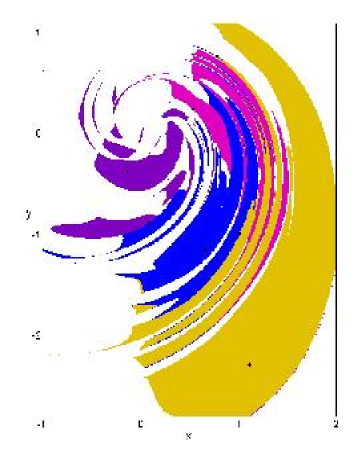
(a) Schur decomposition

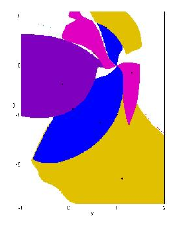
(b) Singular value decomposition

Figure 4.1: Basins of attraction for the period$-3$ orbits of the Ikeda map with parameter values $a=1.0$, $b=0.9$, $k=0.4$ and $\eta=6.0$. Here we have chosen $\tilde{C}=-1$ since in this example the unstable subspace is one-dimensional.

In [62, 88] the Schur decomposition (SchD) SchD is used in order to construct the projectors $P$ and $Q$. This is fine for continuation problems since one may assume from the offset that they possess an initial condition $x_{0}$ sufficiently close to a UPO such that the SchD of $Df(x_{0})$ gives a good approximation to the eigenspace of $Df(x^{*})$. However, it is well known that the eigenvectors of the perturbed Jacobian $Df(x^{*}+\delta x)$ behave erratically as we increase $\delta x$. In order to enlarge the basins of attraction for the UPOs we propose that singular value decomposition (SVD) SVD be used instead. That is we choose an initial condition $x_{0}$ and construct the SVD of its preimage, i.e. $Df(f^{-1}(x_{0}))=USW^{\mathsf{T}}$ (or in the continuous case $D\phi^{T}(\phi^{-T}(x_{0}))=USW^{\mathsf{T}}$ for some time $T$), the columns of $U$ give the stretching directions of the map at $x_{0}$, whilst the singular values determine whether the directions are expanding or contracting. It is these directions which we use to construct the projectors $P$ and $Q$. Due to the robustness of the SVD we expect the respective basins of attraction to increase.

It is not necessary in practice to decompose Eq. (4.13) in order to apply the new ST. Rather we can express $C$ in terms of $\tilde{C}$ and $V_{p}$. To see this we add $V_{q}$ times Eq. (4.17) to $V_{p}$ times Eq. (4.18) to get

$$\frac{dx}{ds} = V_{q}V_{q}^{\mathsf{T}}g(x)+V_{p}\tilde{C}V_{p}^{\mathsf{T}}g(x),$$ (4.19)

$$= [I_{n}+V_{p}(\tilde{C}-I_{n_{u}})V_{p}^{\mathsf{T}}]g(x),$$

where the second line follows from Eq. (4.7). From this we see that the following choice of $C$ is equivalent to the preceding decomposition

$$C=I_{n}+V_{p}(\tilde{C}-I_{n_{u}})V_{p}^{\mathsf{T}}.$$ (4.20)

Thus in practice we compute $V_{p}$ and $\tilde{C}$ at the seed $x_{0}$ in order to construct $C$ and then proceed to solve Eq. (4.14).

The advantage of using the SVD rather than the SchD can be illustrated by the following example. Consider the Ikeda map [50]:

$$f(\mathbf{x}):=\left[\!\!\begin{array}[]{c}x_{i+1}\\ y_{i+1}\end{array}\!\!\right]=\left[\!\!\begin{array}[]{c}a+b(x_{i}\cos{(\phi_{i})}-y_{i}\sin{(\phi_{i})})\\ b(x_{i}\sin{(\phi_{i})}+y_{i}\cos{(\phi_{i})})\end{array}\!\!\right],$$ (4.21)

where $\phi_{i}=k-\eta/(1+x_{i}^{2}+y_{i}^{2})$ and the parameters are chosen such that the map has a chaotic attractor: $a=1.0$, $b=0.9$, $k=0.4$ and $\eta=6.0$. For this choice of parameters the Ikeda map possesses eight period$-3$ orbit points (two period-3 orbits and two fixed points, one of which is on the attractor basin boundary). In our experiments we have covered the attractor for Eq. (4.21) with a grid of initial seeds and solved the associated flow for $p=3$, i.e., $g(x)=f^{3}(x)-x$. This is done twice, firstly in the case where the projections $P$ and $Q$ are constructed via the SchD and secondly when they are constructed through the SVD. Since all UPOs of the Ikeda map are of saddle type, the unstable subspace is one-dimensional and we need only two transformations: $\tilde{C}=1$ and $\tilde{C}=-1$. Figure 4.1 shows the respective basins of attraction for the two experiments with $\tilde{C}=-1$. It can be clearly seen that the use of SVD corresponds to a significant increase in basin size compared to the SchD. Note that with $\tilde{C}=-1$ we stabilise four out of eight fixed points of $f^{3}$. The other four are stabilised with $\tilde{C}=1$. The corresponding basins of attraction are shown in Figure 4.2. Note that for this choice of ST the choice of basis vectors is not important, since Eq. (4.20) yields $C=I$, so that the associated flow is given by Eq. (4.13).

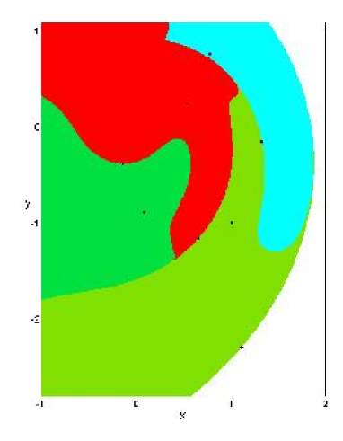
Figure 4.2: The basins of attraction for the Ikeda map for the choice of $\tilde{C}=1$. Fixed points of $f^{3}$ with negative unstable eigenvalues are stable stationary solutions of the associated flow, while those with positive eigenvalues are saddles located at the basin boundaries.

4.2 Implementation

We now wish to apply these ideas to parabolic PDEs of the form (1.14). The numerical solution of such PDEs are typically based upon their representation in terms of a truncated system of nonlinear ODEs. Thus, we will be concerned with the detection of UPOs for large systems of ODEs:

$$\frac{dx}{dt}=v(x),\quad x\in\mathbb{R}^{n},$$ (4.22)

where $v$ is derived from an appropriate discretisation procedure (i.e. finite differences, finite element, spectral method) and $n\gg 1$.

A typical approach in the determination of UPOs for flows is via a Poincaré surface of section (PSS). By “clever” placement of an $(n-1)$-dimensional manifold in the phase space, the problem is reduced to a discrete map defined via intersections with the manifold. However, a correct choice of PSS is a challenging problem in itself. Due to the complex topology of a high-dimensional phase space, the successful detection of UPOs will be highly dependent upon the choice of section. When the choice of a suitable PSS is not obvious a priori, we found it preferable to work with the full flow, adding an auxiliary equation to determine the integration time $T$.

Let $x\mapsto\phi^{t}(x)$ denote the flow map of Eq. (4.22). Then we define the associated flow as follows

$$\frac{dx}{ds} = Cg$$ (4.23)

$$= C(\phi^{T}(x)-x).$$

The additional equation for $T$ is constructed such that $T$ is always changing in the direction that decreases $|\phi^{T}(x)-x|$, i.e.

$$\frac{dT}{ds}\varpropto-\frac{\partial|g|^{2}}{\partial T},$$

or, more precisely

$$\frac{dT}{ds}=-\alpha v(\phi^{T}(x))\cdot(\phi^{T}(x)-x).$$ (4.24)

Here $\alpha>0$ is a constant which controls the relative speed of convergence of Eq. (4.24). This leads to the following augmented flow which must be solved to detect UPOs of (4.22):

$$\frac{d}{ds}\left[\begin{array}[]{c}x\\ T\\ \end{array}\right]=\left[\begin{array}[]{c}C(\phi^{T}(x)-x)\\ -\alpha v(\phi^{T}(x))\cdot(\phi^{T}(x)-x)\\ \end{array}\right].$$ (4.25)

Note that the augmented flow (4.25) is derived by integrating a nonlinear PDE – in our case the KSE – for some time $T$ and will become increasingly stiff for larger $T$.

Several approaches have been proposed for the solution of stiff systems of ODEs; see for example, the review by Shampine and Gear [87]. Of all these techniques the general-purpose codes contained within the ODEPACK software package [44] are regarded as some of the best available routines for the solution of such systems. Thus, in our numerical experiments we use the stiff solver dlsodar from the ODEPACK toolbox to integrate (4.25). dlsodar is a variable step-size solver which automatically changes between stiff and nonstiff modes. In particular, as we approach a steady state of Eq. (4.25) dlsodar will take increasingly larger time-steps, leading to super linear convergence in the neighbourhood of the solution.

To use the solver dlsodar, we must provide a routine that returns the value of the vector field (4.25) evaluated at a given point $(x,T)$. Here we need the solution of Eq. (4.22) which is obtained by applying a suitable numerical integration scheme; see the next section and Appendix .2.7 for further details. The ODEPACK software package makes use of the Jacobian matrix of the system being integrated and provides the option of computing the Jacobian via finite differences or via a user supplied routine. Note that in the case that the flow is expected to be stiff much of the time, it is recommended that a routine for the Jacobian is supplied and we do this. The derivative of (4.25) with respect to $(x,T)$ is given by

$$\left[\begin{array}[]{cc}C(J_{T}-I_{n})&Cv_{T}\\ -\alpha(v_{T}^{\mathsf{T}}(J_{T}-I_{n})+g^{\mathsf{T}}DvJ_{T})&-\alpha(g^{\mathsf{T}}Dvv_{T}+v_{T}^{\mathsf{T}}v_{T})\\ \end{array}\right],$$ (4.26)

where $J_{T}=\partial\phi^{T}(x)/\partial x$, $v_{T}=v(\phi^{T}(x))$, $Dv=dv/dx$ and $g=\phi^{T}(x)-x$ as usual.

Quite often one might wish to terminate simulation before the usual stopping criteria of, for example, a maximum number of steps taken or certain tolerances having been reached. A useful feature of the dlsodar algorithm is that it allows the optional user supplied routine to do just this. To be more exact, it determines the roots of any of a set of user supplied functions

$$h_{i}=h_{i}(t,x_{1},\dots,x_{n}),\quad i=1,\dots,m,$$

and returns the solution of (4.25) at the root if it occurs prior to the normal stopping criteria.

Note that, to increase the efficiency of the algorithm we wish to avoid the following two instances: firstly, due to the local nature of the STs, we should stop the search if we wander too far from the initial condition, and secondly, since our search is governed by the dynamics of Eq. (4.23) and not by those of (4.22), we might move off the attractor after some time period so the convergence to a UPO becomes highly unlikely. In our numerical experiments we supply the following function

$$h_{1}=a-|g|,$$ (4.27)

where $a\in\mathbb{R}$ is a constant and $|\cdot|$ denotes the $L_{2}$ norm. In practice, we have found that there exists a threshold value of $a$, such that convergence is highly unlikely once the norm of $g$ surpasses it. Note that we also restrict the maximum number of allowed integration steps since the convergence becomes less likely if the associated flow is integrated for a long time.

We must also provide two tolerances, rtol and atol, which control the local error of the ODE solver. In particular, the estimated local error in $X=(x,T)$ will be controlled so as to be less than

$$\mathrm{rtol}\cdot||X||_{\infty}+\mathrm{atol}.$$

Thus the local error test passes if, in each component, either the absolute error is less than atol or the relative error is less than rtol. The accuracy with which we would like to solve the flow (4.25) is determined by the stability properties of (4.22). To understand this, we note that in evaluating the RHS of (4.25) it is the solution of Eq. (4.22) at time $T$, i.e. $\phi^{T}(x)$, which is critical for error considerations. Suppose that our initial point lies within $\delta x$ of a true trajectory $x$. Then $\phi^{T}(x+\delta x)$ lies approximately within $e^{\lambda T}\delta x$ of the true trajectory, $\phi^{T}(x)$, where $\lambda$ is the largest Lyapunov exponent of the system. Since $\lambda$ is positive for chaotic systems, the error grows exponentially with the period and we should take this into account when setting the tolerances rtol and atol. This leads us to the following settings for the tolerances

$$\mathrm{rtol}=\mathrm{atol}=10^{-5}/e^{\lambda T_{0}},$$ (4.28)

where $T_{0}$ is the initial period and $\lambda$ is the largest Lyapunov exponent of the flow $v$. We have computed the Lyapunov exponent using the algorithm due to Benettin et al [2]; see Appendix .2.7 for a description of the routine as well as a brief review of Lyapunov exponents.

4.2.1 Kuramoto-Sivashinsky equation

We have chosen the Kuramoto-Sivashinsky equation (KSE)KSE for our numerical experiments. It is the simplest example of spatiotemporal chaos and has been studied in a similar context in [9, 57, 100], where the detection of many UPOs has been reported. We work with the KSE in the form

$$u_{t}=-\frac{1}{2}(u^{2})_{x}-u_{xx}-u_{xxxx},$$ (4.29)

where $x\in[0,L]$ is the spatial coordinate, $t\in\mathbb{R}^{+}$ is the time and the subscripts $x$, $t$ denote differentiation with respect to space and time. For $L<2\pi$, $u(x,t)=0$ is the global attractor for the system and the resulting long time dynamics are trivial. However, for increasing $L$ the system undergoes a sequence of bifurcations leading to complicated dynamics; see for example [54].

Our setup will be close to that found in [57]. In what follows we assume periodic boundary conditions: $u(x,t)=u(x+L,t)$, and restrict our search to the subspace of antisymmetric solutions, i.e. $u(x,t)=-u(L-x,t)$. Due to the periodicity of the solution, we can solve Eq. (4.29) using the pseudo-spectral method [36, 94]. Representing the function $u(x,t)$ in terms of its Fourier modes:

$$\quad u(x,t):={\cal F}^{-1}[\hat{u}]=\sum_{k\in{\mathbb{Z}}}\hat{u}_{k}e^{-ikqx},$$ (4.30)

where

$$\hat{u}:=(\dots,\hat{u}_{-1},\hat{u}_{0},\hat{u}_{1},\dots)^{\mathsf{T}}\,,\qquad\hat{u}_{k}:={\cal F}[u]_{k}=\frac{1}{L}\int_{0}^{L}u(x,t)e^{ikqx}dx,$$ (4.31)

we arrive at the following system of ODEs

$$\frac{d\hat{u}_{k}}{dt}=[(kq)^{2}-(kq)^{4}]\hat{u}_{k}+\frac{ikq}{2}{\cal F}[({\cal F}^{-1}[\hat{u}])^{2}]_{k}\,.$$ (4.32)

Here $q=2\pi/L$ is the basic wave number. Since $u$ is real, the Fourier modes are related by $\hat{u}_{-k}=\hat{u}^{\ast}_{k}$. Furthermore, since we restrict our search to the subspace of odd solutions, the Fourier modes are pure imaginary, i.e. $\mathfrak{Re}(\hat{u}_{k})=0$.

The above system is truncated as follows: the Fourier transform ${\cal F}$ is replaced by its discrete equivalent

$$a_{k}:={\cal F}_{N}[u]_{k}=\sum_{j=0}^{N-1}u(x_{j})e^{ikqx_{j}}\,,\qquad u(x_{j}):={\cal F}_{N}^{-1}[a]_{j}=\frac{1}{N}\sum_{k=0}^{N-1}a_{j}e^{-ikqx_{j}}\,,$$ (4.33)

where $x_{j}=L/N$ and $a_{N-k}=a^{\ast}_{k}$. Since $a_{0}=0$ due to Galilean invariance and setting $a_{N/2}=0$ (assuming $N$ is even), the number of independent variables in the truncated system is $n=N/2-1$. The truncated system looks as follows:

$$\dot{a}_{k}=[(kq)^{2}-(kq)^{4}]a_{k}+\frac{ikq}{2}{\cal F}_{N}[({\cal F}_{N}^{-1}[a])^{2}]_{k}\,,$$ (4.34)

with $k=1,\ldots,n$, although in the Fourier transform we need to use $a_{k}$ over the full range of $k$ values from 0 to $N-1$.

The discrete Fourier transform ${\cal F}_{N}$ can be computed using fast Fourier transform (FFT).FFT In Fortran and C, the routine REALFT from Numerical Recipes [77] can be used. In Matlab, it is more convenient to use complex variables for $a_{k}$. Note that Matlab function fft is, in fact, the inverse Fourier transform.

To derive the equation for the matrix of variations, we use the fact that ${\cal F}_{N}$ is a linear operator to obtain

$$\frac{\partial\dot{a}_{k}}{\partial a_{j}}=[(kq)^{2}-(kq)^{4}]\delta_{kj}+ikq{\cal F}_{N}[{\cal F}_{N}^{-1}[a]\otimes{\cal F}_{N}^{-1}[\delta_{kj}]]\,,\quad j=1,\ldots,n,$$ (4.35)

where $\otimes$ indicates componentwise product, and the inverse Fourier transform is applied separately to each column of $\delta_{kj}$. Here, $\delta_{kj}$ is not a standard Kronecker delta, but the $N\times n$ matrix:

$$\delta_{kj}=\left(\begin{array}[]{ccc}0&0&\cdots\\ 1&0&\cdots\\ 0&1&\cdots\\ \lx@intercol\dotfill\hfil\hfil\lx@intercol\\ 0&0&\cdots\\ \lx@intercol\dotfill\hfil\hfil\lx@intercol\\ 0&-1&\cdots\\ -1&0&\cdots\\ \end{array}\right),$$ (4.36)

with index $k$ running from 0 to $N-1$.

In practice the number of degrees of freedom $n$ should be sufficiently large so that no modes important to the dynamics are truncated, whilst on the other hand, an increase in $n$ corresponds to an increase in computation. To determine the order of the truncation in our numerical experiments, we initially chose $n$ to be large and integrated a random initial seed onto the attractor. By monitoring the magnitude of the harmonics an integer $k$ was determined such that $a_{j}<10^{-5}$ for $j>k$. The value of $n$ was then chosen to be the smallest integer such that: (i) $n\geq k$, and (ii) $N=2n+2$ was an integer power of two. The second condition ensures that the FFT is applied to vectors of size which is a power of two resulting in optimal performance.

Note that in the numerical results to follow we work entirely in Fourier space and use the ETDRK4 time-stepping to solve (4.34) and (4.35); for further details concerning the method of exponential-time-differencing see Appendix .2.7. In particular the method uses a fixed step-size ($h=0.25$ in our calculations) thus it is necessary to use an interpolation scheme in order to integrate up to arbitrary times. In our work we have implemented cubic interpolation [77]. More precisely, to integrate up to time $t\in[t_{i},t_{i}+h]$, where the $t_{i}$ are integer multiples of the step-size $h$. We construct the unique third order polynomial passing through the two points $a(t_{i})$ and $a(t_{i}+h)$, with derivatives $a^{\prime}(t_{i})$ and $a^{\prime}(t_{i}+h)$ at the respective points. In this way we obtain the following cubic model:

$$p(s)=[ \,2a(t_{i})+a^{\prime}(t_{i})+a^{\prime}(t_{i}+h)-2a(t_{i}+h)]s^{3}+[3a(t_{i}+h)-3a(t_{i})$$

$$-2a^{\prime}(t_{i})-a^{\prime}(t_{i}+h)]s^{2}+a^{\prime}(t_{i})s+a(t_{i}),$$ (4.37)

where the parameter $s=(t-t_{i})/h\in[0,1]$.

4.2.2 Numerical results

We now present the results of our numerical experiments. We begin with a comparison between our method and the nonlinear least squares solver lmder from the MINPACK software package [66]. Note that lmder is an implementation of the Levenburg-Marquardt algorithm – see §2.3. We have chosen it because it has recently been applied successfully to detect many UPOs of the closely related complex Ginzburg-Landau equation.

In order to determine UPOs via the lmder routine we introduce the following augmented system

$$F(x,T)=\left[\begin{array}[]{c}\phi^{T}(x)-x\\ v(\phi^{T}(x))\cdot(\phi^{T}(x)-x)\\ \end{array}\right]=0,$$ (4.38)

where the second equation is motivated in analogous fashion to the auxiliary equation (4.24). To use the lmder solver we must provide a routine that returns the value of $F$ evaluated at a given point $(x,T)$. Also, we provide a routine to compute the Jacobian analytically rather than use finite differences, the formula of which differs from Eq. (4.26) only by multiplication by a constant matrix. In addition to this the user must supply three tolerances: ftol, xtol, and gtol. Here, ftol measures the relative error desired in the sum of squares, xtol the relative error desired in the approximate solution, and gtol measures the orthogonality desired between the vector function $F$ and the columns of the Jacobian. In the computations performed in the next section we set the tolerances to the recommended values:

$$\mathrm{ftol}=10^{-8},\quad\mathrm{xtol}=10^{-8}\quad\mathrm{and}\quad\mathrm{gtol}=0.$$

Finally, we specify a maximum number of function evaluations allowed during each run of the lmder algorithm in order to increase its efficiency.

For our method we use the set of matrices proposed in §4.1.1 with

$$\tilde{C}=\mathcal{C}_{\mathrm{SD}},$$ (4.39)

since within the low-dimensional unstable subspace it is possible to apply the full set of Schmelcher-Diakonos (SD) matrices. The UPOs determined from our search will then be used as seeds to determine new cycles. Here we proceed in analogous fashion to Chapter 3 by constructing STs from the monodromy matrix, $D\phi^{T^{*}}(a^{*})$, of the cycle $(a^{*},T^{*})$. We then solve the augmented flow (4.25) from the new initial condition $(a^{*},\tilde{T})$, where the time $\tilde{T}$ is chosen such that

$$a^{*}(0)\approx a^{*}(\tilde{T}),\quad\mathrm{and}\quad\tilde{T}\leavevmode\nobreak\ (\mathrm{mod}T^{*})\neq 0.$$ (4.40)

Note that any given cycle may exhibit many close returns, particularly longer cycles, thus in general a periodic orbit may produce many new initial seeds. This is an especially useful feature, since we do not have to recompute the corresponding STs.

Initially, to determine that a newly detected cycle, $(x^{*},T^{*})$, was different from those already found, we first checked whether the periods differed, that is, we determined whether $|T^{*}-T^{\prime}|>T_{\mathrm{tol}}$ for all previously detected orbits. If two orbits where found to have the same period, we then calculated the distance between the first components of $x^{*}$, and all other detected orbits $y^{*}$. However, in practice we found, that if two orbits have the same period, then either they are the same or they are related via symmetry, recall that if $u(x,t)$ is a solution then so is $-u(L-x,t)$. Thus, in order to avoid the convergence of UPOs that are trivially related by symmetry we will consider two orbits as being equal if their periods differ by less than the tolerance $T_{\mathrm{tol}}$. Of course, this criterion can, in theory, lead us to discard cycles incorrectly, however, this is highly unlikely in practice.

Stabilising transformations vs Levenberg-Marquardt

The search for UPOs is conducted within a rectangular region containing the chaotic invariant set. Initial seeds are obtained by integrating a random point within the region for some transient time $\tau$. Once on the attractor, the search for close returns within chaotic dynamics is implemented. That is, we integrate the system from the initial point on the attractor until $a(t_{0})\approx a(t_{1})$ for some times $t_{0}<t_{1}$, and use the close return, $(a(t_{0}),T_{0})$, where $T_{0}=t_{1}-t_{0}$, as our initial guess to a time-periodic solution. In order to build the STs we solve the variational equations for each seed starting from the random initial point, $a(0)$, for time $\tau+t_{0}$. In order to construct the matrix $V_{p}$, we apply the SVD to the matrix

$$D\phi^{\tau+t_{0}}(a(0))=USW^{\mathsf{T}},$$ (4.41)

the corresponding ST is given by

$$C=I_{n}+V_{p}(\tilde{C}-I_{n_{u}})V_{p}^{\mathsf{T}},$$ (4.42)

where $V_{p}=U_{jk}$, $j=1,\dots,n$, $k=1,\dots,n_{u}$, i.e. the first $n_{u}$ columns of $U$ in (4.41). Here $n_{u}$ is the number of expanding directions which is determined by the number of singular values with modulus greater than one.

Table 4.1: The number of distinct periodic solutions for the Kuramoto-Sivashinsky equation detected by the method of STs. Here $L=38.5$ and $\alpha=0.25$.

Period	C	$N_{\mathrm{po}}$	$N_{\mathrm{hit}}$	$N_{\mathrm{fev}}$	$N_{\mathrm{jev}}$	Work
$10-100$	$C_{0}$	$28$	$498$	$252$	$10$	$412$
	$C_{1}$	$16$	$296$	$684$	$32$	$1196$
	$\{C_{i}\}$	$44$	$794$	$936$	$42$	$1608$
$100-250$	$C_{0}$	$235$	$395$	$903$	$78$	$2151$
	$C_{1}$	$64$	$256$	$1294$	$112$	$3086$
	$\{C_{i}\}$	$299$	$651$	$2197$	$190$	$5237$

Table 4.2: The number of distinct periodic solutions for the Kuramoto-Sivashinsky equation detected by the Levenberg-Marquardt algorithm lmder with $L=38.5$.

Period	$N_{\mathrm{po}}$	$N_{\mathrm{hit}}$	$N_{\mathrm{fev}}$	$N_{\mathrm{jev}}$	Work
$10-100$	$42$	$497$	$20$	$15$	$260$
$100-250$	$208$	$291$	$500$	$452$	$7732$

We examine two different system sizes: $L=38.5$, for which the detected UPOs typically have one positive Lyapunov exponent, and $L=51.4$, for which the UPOs have either one or two positive Lyapunov exponents. The corresponding systems sizes are $n=15$ and $n=31$ respectively. Our experiments where conducted over two separate ranges. We began by looking for shorter cycles with period $T\in[10,100]$, the lower bound here was determined a posteriori so as to be smaller than the shortest detected cycle. We then searched for longer cycles, $T\in[100,250]$ to be more precise, where the maximum of $T=250$ was chosen in order to reduce the computational effort.

In our calculations we set the positive constant $\alpha=0.25$ in Eq. (4.25). Using the solver dlsodar we integrated $500$ random seeds over both ranges for time $s=150$, the seeds where chosen such that $|\phi^{T_{0}}(a(0))-a(0)|<1.0$. If the flow did not converge within $1000$ integration steps, we found it more efficient to terminate the solver and to re-start with a different ST or a new seed. As mentioned in the previous section we choose a constant $a=50$ experimentally so that integration is terminated if the norm of $g$ grows to large, i.e. $|g(x)|=|\phi^{T}(x)-x|>a$.

Typically on convergence of the associated flow the UPO is determined with accuracy of about $10^{-7}$ at which point we implement two or three iterations of the Newton-Armijo rule to the following system

$$\left(\begin{array}[]{cc}M_{T}-I_{n}&v(\phi^{T}(x))\\ v(x)&0\\ \end{array}\right)\left(\begin{array}[]{c}\delta x\\ \delta T\\ \end{array}\right)=-\left(\begin{array}[]{c}\phi^{T}(x)-x\\ 0\\ \end{array}\right),$$ (4.43)

in order to allow convergence to a UPO to within roundoff error. The linear system (4.43) was introduced by Zoldi and Greenside [100] as a method for determining UPOs for extended systems in its own right, and in particular, has been applied successfully in the detection of UPOs for the KSE.

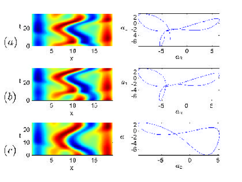
Figure 4.3: Illustration of two UPOs of KSE detected from a single seed. We show both a level plot for the solutions and a projection onto the first two Fourier components. Since $u(x,t)$ is antisymmetric on $[0,L]$, it is sufficient to display the space-time evolution of $u(x,t)$ on the interval $[0,L/2]$: (a) Seed with time $T=37.0$, (b) a periodic solution of length $T=36.9266$ detected with stabilising transformation $\tilde{C}=+1$ and (c) a periodic solution of length $T=25.8489$ detected with stabilising transformation $\tilde{C}=-1$.

Table 4.3: The number of distinct periodic solutions for the Kuramoto-Sivashinsky equation detected by the method of stabilising transformations. Here $L=51.4$ and $\alpha=0.25$.

Period	C	$N_{\mathrm{po}}$	$N_{\mathrm{hit}}$	$N_{\mathrm{fev}}$	$N_{\mathrm{jev}}$	Work
$10-100$	$C_{0}$	$11$	$366$	$382$	$16$	$894$
	$C_{1}$	$1$	$221$	$410$	$23$	$1146$
	$C_{2}$	$7$	$108$	$456$	$20$	$1096$
	$C_{3}$	$2$	$81$	$357$	$13$	$773$
	$C_{4}$	$2$	$157$	$464$	$26$	$1296$
	$C_{5}$	$0$	$171$	$654$	$35$	$1774$
	$C_{6}$	$5$	$174$	$666$	$36$	$1818$
	$C_{7}$	$2$	$139$	$496$	$36$	$1648$
	$\{C_{i}\}$	$30$	$1417$	$3885$	$205$	$10445$
$100-250$	$C_{0}$	$51$	$330$	$628$	$17$	$1172$
	$C_{1}$	$7$	$209$	$807$	$27$	$1671$
	$C_{2}$	$17$	$138$	$936$	$31$	$1928$
	$C_{3}$	$21$	$177$	$917$	$26$	$1749$
	$C_{4}$	$11$	$161$	$877$	$36$	$2029$
	$C_{5}$	$0$	$116$	$960$	$43$	$2336$
	$C_{6}$	$1$	$117$	$975$	$42$	$2319$
	$C_{7}$	$6$	$161$	$879$	$35$	$1999$
	$\{C_{i}\}$	$114$	$1409$	$6979$	$257$	$15203$

Table 4.4: The number of distinct periodic solutions for the Kuramoto-Sivashinsky equation detected by the Levenberg-Marquardt algorithm lmder with $L=51.4$.

Period	$N_{\mathrm{po}}$	$N_{\mathrm{hit}}$	$N_{\mathrm{fev}}$	$N_{\mathrm{jev}}$	Work
$10-100$	$20$	$480$	$64$	$52$	$1728$
$100-250$	$86$	$356$	$374$	$332$	$10998$

Similarly, we run the lmder routine from the same $500$ seeds over the two different time ranges. The routine terminates if one of the following three scenarios arise: (i) a predefined maximum number of function evaluations is exceeded, we set the maximum number of function evaluations equal to $1000$, (ii) the error between two consecutive steps is less than xtol, but the sum of squares is greater than ftol, indicating a local minimum has been detected, or (iii) both xtol and ftol are satisfied indicating that convergence to a UPO has been obtained.

In order to make a comparison between the efficiency of the two methods we introduce the measure of the work done per seed:

$$\mathrm{Work}=N_{\mathrm{fev}}+n\times N_{\mathrm{jev}}.$$ (4.44)

Here $N_{\mathrm{fev}}$ is the average number of function evaluations per seed, $N_{\mathrm{jev}}$ the average number of Jacobian evaluations per seed and $n$ is the size of the system being solved. The expression in (4.44) takes into account the fact that evaluation of the Jacobian is $n$ times more expensive than evaluation of the function itself.

We present the results of our experiments in Tables 4.1 – 4.4. Here $N_{\mathrm{po}}$ denotes the number of distinct orbits found, $N_{\mathrm{hit}}$ gives the number of times we converged to a UPO, and $N_{\mathrm{fev}}$, $N_{\mathrm{jev}}$, and Work, are as defined above. In Tables 4.1 and 4.3 the performance of the stabilising transformations are analysed both collectively and on an individual basis; here the different $C_{i}$ denote the different SD matrices. In Table 4.1 $C_{0}=+1$ and $C_{1}=-1$, whilst in Table 4.3 we have

$$\left\{C_{0}=\left[\begin{array}[]{cc}1&0\\ 0&1\\ \end{array}\right],\right.C_{1}=\left[\begin{array}[]{cc}-1&0\\ 0&1\\ \end{array}\right],C_{2}=\left[\begin{array}[]{cc}1&0\\ 0&-1\\ \end{array}\right],C_{3}=\left[\begin{array}[]{cc}-1&0\\ 0&-1\\ \end{array}\right],$$

$$C_{4}=\left[\begin{array}[]{cc}0&1\\ 1&0\\ \end{array}\right],C_{5}=\left[\begin{array}[]{cc}0&-1\\ 1&0\\ \end{array}\right],C_{6}=\left[\begin{array}[]{cc}0&1\\ -1&0\\ \end{array}\right],\left.C_{7}=\left[\begin{array}[]{cc}0&-1\\ -1&\\ \end{array}\right]\right\}$$

The total work done per seed is given by the sum over all the SD matrices and is denoted by $\{C_{i}\}$.

For $L=38.5$ we detected a total of $343$ UPOs using the ST method as compared to $250$ UPOs using the lmder algorithm, whilst for $L=51.4$ we found $144$ and $106$ UPOs with the respective methods. Both methods found roughly the same number of orbits when searching for shorter period cycles. However, as can be seen by comparing the work done per seed in Tables 4.1 – 4.4 lmder performs better than the ST method in that case. The situation changes, however, when we look at the detection of longer cycles. For $L=38.5$ in particular, we see that the ST method computes many more orbits with a considerable reduction in the cost. In fact, using the identity matrix alone, the ST method detects more UPOs than lmder at approximately a quarter of the cost. For larger system size, $L=51.4$, the ST method still detects more orbits than lmder. However, in doing so a considerable amount of extra work is done. It is important to note here, that the increase in work is not due to any deficiency in the ST method. Rather, the rise in the computational cost is brought about due to the fact that not all the SD matrices work well. For example, the subset of matrices $\{C_{0},C_{2},C_{3},C_{4}\}\subset\mathcal{C}_{\mathrm{SD}}$, detect approximately $90\%$ of the longer period UPOs, yet they account for less than $50\%$ of the overall work. Indeed, for this particular choice of matrices the ST method still detects more orbits, but more importantly, its performance now exceeds that of lmder.

Note that it is not surprising that the SD matrices do not perform equally well, this is, after all, what we would have expected based upon our experience with maps. However, it is still important to try all SD matrices – when possible – in order to compare their efficiency, especially if one wishes to construct minimal sets of ST matrices.

For detecting longer period orbits the performance of lmder suffers due to the large increase in the number of Jacobian evaluations needed; see Tables 4.2 and 4.4. Recall, that lmder is an implementation of the Levenberg-Marquardt algorithm, and that in particular, it computes the Jacobian once on each iterate. Thus, we may view the number of Jacobian evaluations as the number of steps required in order to converge. The increase in the number of iterations necessary to obtain convergence can be understood by considering the dependance of $|\phi^{T}(x)-x|$ on x. For increasing period the level curves of $|g|^{2}$ are squeezed along the unstable manifold of $\phi^{T}(x)$, resulting in a complicated surface with many minima, both local and global, embedded within long, winding, narrow “troughs”. Note that this is a common problem with all methods that use a cost function to obtain “global” convergence, since these methods only move in the direction that decreases the cost function.

This can be explained by the following heuristics: for simplicity let us assume that we are dealing with a map $x_{n+1}=f(x_{n})$, whose unstable manifold is a one-dimensional object. In that case, we may define a one-dimensional map, locally, about a period-p orbit, $x^{*}$, of the map $f$ as

$$\bar{h}(s)=|g(x^{*}+\delta x)|^{2}.$$ (4.47)

Here $g=f^{p}(x)-x$ as usual, $\delta x=x(s)-x^{*}$ is small, and we only allow $x(s)$ to vary along the unstable manifold. Expanding $g$ in a Taylor series about the periodic orbit, $x^{*}$, we obtain

$$\bar{h}(s) = |g(x^{*})+Dg(x^{*})\delta x+O(\delta x^{2})|^{2}$$

$$= |(Df^{p}(x^{*})-I_{n})\delta x+O(\delta x^{2})|^{2}$$

$$= \delta x^{\mathsf{T}}(\Lambda^{p}-I_{n})^{2}\delta x+O(\delta x^{3}),$$

where the third line follows since $\delta x$ is an eigenvector of $Df(x^{*})$ with corresponding eigenvalue $\lambda$, and $\Lambda=\mathrm{diag}(\lambda,\dots\lambda)$. Note that in the above we assume that $p$ is large but finite so that the term $(\Lambda^{p}-I_{n})^{2}$ remains bounded. Now, close to the periodic orbit, $\bar{h}$ is approximately a quadratic form with slope of the order $\lambda^{p}$, and since $|\lambda|>1$, it follows that if we move along the unstable manifold $|g|^{2}$ will grow quicker for larger periods, or, in other words, the level curves are compressed along the unstable direction.

Since the lmder algorithm reduces the norm of $f$ at each step, it will typically follow the gradient to the bottom of the nearest trough, where it will start to move along the narrow base towards a minimum. Once at the base of a trough, however, lmder is forced into taking very small steps, this follows due to the nature of the troughs, i.e. the base is extremely narrow and winding, and since lmder chooses its next step-size based on the straight line search. One of the benefits of the ST method is that it does not need to decrease the norm at each step and thus, does not suffer from such considerations.

Another advantage of our method is that we can converge to several different UPOs from just one seed, depending upon which ST is used. Figure 4.3 shows one of such cases, where Eq. (4.25) is solved from the same seed for each of the $2^{n_{u}}$ STs ($n_{u}=1$ in this example), with two of them converging to two different UPOs. Figure 4.3a shows the level plot of the initial condition and a projection onto the first two Fourier components. Figures 4.3b and 4.3c show two unstable spatiotemporally periodic solutions which where detected from this initial condition, the first of period $T=36.9266$ was detected using $\tilde{C}=+1$, whilst the second of period $T=25.8489$ was detected using $\tilde{C}=-1$. The ability to detect several orbits from one seed increases the efficiency of the algorithm.

Seeding with UPOs

Table 4.5: Number of distinct orbits detected using the method of stabilising transformations with periodic orbits as seeds The number of seeds is $489$. $L=38.5$, $\alpha=0.25$.

C	$N_{\mathrm{po}}$	$N_{\mathrm{hit}}$	$N_{\mathrm{fev}}$	$N_{\mathrm{jev}}$	Work
$C_{0}$	$46$	$209$	$2814$	$136$	$4854$
$C_{1}$	$52$	$198$	$2819$	$130$	$4769$
$\{C_{i}\}$	$98$	$407$	$5633$	$266$	$9623$

Table 4.6: Number of distinct orbits detected using the method of stabilising transformations with periodic orbits as seeds. The number of seeds is $123$. $L=51.4$, $\alpha=0.25$.

C	$N_{\mathrm{po}}$	$N_{\mathrm{hit}}$	$N_{\mathrm{fev}}$	$N_{\mathrm{jev}}$	Work
$C_{0}$	$1$	$21$	$2797$	$48$	$4333$
$C_{1}$	$2$	$37$	$2815$	$40$	$4095$
$C_{2}$	$0$	$0$	$216$	$3$	$312$
$C_{3}$	$0$	$1$	$187$	$2$	$251$
$\{C_{i}\}$	$3$	$59$	$6015$	$93$	$8691$

In order to construct a seed from an already detected orbit, $(a^{*},T^{*})$, we begin by searching for close returns. That is, starting from a point on the orbit, $a^{*}(t_{0})$, we search for a time $t_{1}$ such that $a(t_{1})$ is close to $a(t_{0})$. As long as $\tilde{T}\mathrm{mod}T\neq 0$, where $\tilde{T}=t_{1}-t_{0}$, we take $(a^{*}(t_{0}),\tilde{T})$ as our initial guess to a time periodic solution. For longer period cycles, we can find many close returns by integrating just once over the period of the orbit. Shorter cycles, however, produce fewer recurrences and, in general, must be integrated over longer times to find good initial seeds. In our experiments we searched for close returns $\tilde{T}\in(10,2T^{*})$ if $T^{*}<150.0$; otherwise, we chose $\tilde{T}\in(10,T^{*})$.

Stabilising transformations are constructed by applying the polar decomposition to the matrix $\tilde{G}=\tilde{Q}\tilde{B}$, where $\tilde{G}$ is defined by

$$\tilde{G}:=V(S\Lambda-\mathrm{I}_{n})V^{-1}.$$

Here $V$ and $\Lambda$ are defined through the eigen decomposition of $D\phi^{T^{*}}(a^{*}(t_{0}))=V\Lambda V^{-1}$, and $S=\mathrm{diag}(\pm 1,\pm 1,\ldots,\pm 1)$. The different transformations are then given by $C=-\tilde{Q}^{\mathsf{T}}$. Recall from Chapter 3 that changing the signs of the stable eigenvalues is not expected to result in a substantially different stabilising transformation, thus we use the subset of $S$ such that $S_{ii}=1$ for $i>n_{u}$. For $L=38.5$, we have just two such transformations, since all periodic orbits have only one unstable eigenvalue. Whilst for $L=51.4$, we will have either two or four transformations depending upon the number of unstable eigenvalues of $D\phi^{T^{*}}(a^{*}(t_{0}))$.

In the calculations to follow, a close return was accepted if $|a^{*}(t_{1})-a^{*}(t_{0})|<2.5$. Note that, this was the smallest value to produce a sufficient number of recurrences to initiate the search. A particular cycle may exhibit many close returns. In the following, we set the maximum number of seeds per orbit equal to $5$. To obtain convergence within tolerance $10^{-7}$ we had to increase the integration time to $s=250$ and the maximum number of integration steps allowed to $2000$. If we converged to a UPO then as in the preceding section, we apply two or three Newton-Armijo steps to the linear system (4.43) in order to converge to machine precision.

The results of our experiments are given in Tables 4.5 and 4.6. As in the previous section, $N_{\mathrm{po}}$ denotes the number of distinct orbits found, $N_{\mathrm{hit}}$ the number of times we converged to a UPO, $N_{\mathrm{fev}}$ the average number of function evaluations per seed, and $N_{\mathrm{jac}}$ the average number of jacobian evaluations per seed. The computational cost per seed is measured in terms of the average number of function evaluations per seed and is defined as in Eq. (4.44). In Tables 4.5 and 4.6 the different $C_{i}$ can be uniquely identified by the signature of pluses and minuses defined through the corresponding matrix $S$. For $L=38.5$, the matrices $C_{0}$ and $C_{1}$ correspond to the signatures $(+,\ldots,+)$ and $(-,+,\ldots,+)$, respectively, whilst for $L=51.4$, the matrices $C_{0}$, $C_{1}$, $C_{2}$ and $C_{3}$ correspond to $(+,\ldots,+)$, $(-,+,\ldots,+)$, $(-,-,+,\ldots,+)$, and $(+,-,\ldots,+)$ respectively. As before, the total work done per seed is defined as the sum over all matrices and is denoted by $\{C_{i}\}$.

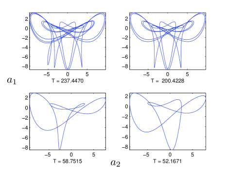
Figure 4.4: Illustration of how a UPO can be used as a seed to detect new cycles. We show the projection onto the first two Fourier components of the initial seed ($T=237.4470$) and the three detected orbits. Here $L=38.5$ and $n=15$.

For $L=38.5$ we where able to construct $489$ seeds from $343$ previously detected periodic orbits. From the new seeds we found a further $98$ distinct UPOs, bringing the total number of distinct orbits detected for $L=38.5$ to $433$. An important observation to make is that both matrices perform equally well, as can be seen from Table 4.5. This is in contrast to the SD matrices for which the performance of the different matrices varies greatly; see Tables 4.1 and 4.3. The result of using periodic orbits as seeds has, however, increased the cost per seed as compared with the cost of seeding with close returns within a chaotic orbit, see Tables 4.1 and 4.5. The increased computation is due mainly to the fact that the close returns obtained from periodic orbits are not as good as those obtained from a chaotic orbit. Recall that the stabilising transformations are based on the local invariant directions of the orbit, and we would expect the performance to suffer as we move further from the seed.

For larger system size, where the system becomes more chaotic, the construction of seeds from close returns becomes increasingly difficult. For $L=51.4$, we constructed $123$ initial seeds from the $144$ periodic orbits using the method of near recurrences. Here we detected only $3$ new distinct UPOs. It is important to note, however, that although we do not find many new UPOs for the case $L=51.4$, the method is still converging for approximately $20\%$ of all initial seeds. Also, in Table 4.6, the poor performance of the matrices $C_{2}$, $C_{3}$ as compared to that of $C_{0}$, $C_{1}$, is due to the fact that only a small percentage of seeds were constructed from orbits with two positive Lyapunov exponents.

One advantage of using periodic orbits as seeds is that we can construct many seeds from a single orbit. Figure 4.4 gives an illustration of three periodic orbits which were detected from a long periodic orbit used as seed. Figure 4.4 shows the projection onto the first two Fourier components of the initial seed (of period $T=237.4470$) and the three orbits detected whose periods in descending order are $T=200.428$, $T=58.7515$ and $T=52.1671$. For each seed determined from a particular periodic orbit the stability transformations are the same. Hence, the ability to construct several seeds from a single orbit, increases the efficiency of the scheme.

4.3 Summary

In this chapter we have presented a scheme for detecting unstable periodic orbits (UPOs) in high-dimensional chaotic systems [13, 15] based upon the stabilising transformations (STs) proposed in [19, 83]. Due to the fact that high-dimensional systems studied in dynamical systems typically consist of low-dimensional dynamics embedded within a high-dimensional phase space, it is possible to increase the efficiency of the STs approach by restricting the construction of such transformations only to the low-dimensional unstable subspace. Following the approach often adopted in subspace iteration methods [62], we construct a decomposition of the tangent space into unstable and stable orthogonal subspaces. We find that the use of singular value decomposition to approximate the appropriate subspaces is preferable to that of Schur decomposition, which is usually employed within the subspace iteration approach. As illustrated with the example of the Ikeda map, the decomposition based on singular value decomposition is less susceptible to variations in the properties of the tangent space away from a seed and thus produce larger basins of attraction for stabilised periodic orbits. Within the low-dimensional unstable subspace, the number of useful STs is relatively small, so it is possible to apply the full set of Schmelcher-Diakonos matrices. The detected orbits were then used as seeds in order to search for new UPOs, thus enabling us to apply the STs introduced in [14].

Chapter 5 Summary and outlook

In mathematics you don’t understand things. You just get used to them.
J. von Neumann

5.1 Summary

In this thesis we have discussed in detail the application to high-dimensional systems of the method of stabilising transformations (ST). The main advantage of the ST approach as compared to other methods is its excellent convergence properties. In particular, the basins of attraction are much larger than the basins produced by other iterative schemes, and are simply connected regions in phase space. The convergence properties for methods of Newton or secant type, can be improved upon by using a line search, the step-size being determined by a suitable cost function. However, such methods have no way of differentiating between true roots and local minima of the cost function; a problem which increases significantly with system dimension due to the topology of multi-dimensional flows.

The application to high-dimensional systems however, is not straightforward. The set of transformations conjectured by Schmelcher and Diakonos (SD) have two major failings: (i) the complete set of transformations has cardinality $2^{n}n!$ (here $n$ is the system dimension), and (ii) this set contains a certain redundancy, in that, not all matrices are useful. The main focus has been on trying to understand the theoretical foundations of the stabilising transformations in order to determine a new minimal set of such transformations enabling efficient detection for systems with $n\geq 4$.

Our approach is based on the understanding of the relationship between the stabilising transformations and the properties of the eigenvalues and eigenvectors of the stability matrices of the periodic orbits. Of particular significance is the observation that only the unstable eigenvalues are important for determining the stabilisation matrices. Therefore, unlike the SD matrices, whose numbers grow with system dimensionality as $2^{n}n!$, our set has at most $2^{k}$ elements, where $k$ is the dimension of the unstable manifold. The dependence of the number of transformations on the dimensionality of the unstable manifold is especially important in cases when we study low-dimensional chaotic dynamics embedded within a high-dimensional phase space.

The ST method was originally developed for the detection of periodic orbits in time-discrete maps. However, the periodic orbits can be used similarly to infer the properties of time-continuous dynamical systems. Here, the ST approach is typically applied directly to the corresponding Poincaré map, where the Poincaré surface of section (PSS) can be a stroboscopic map or defined in terms of phase space intersections. For high-dimensional systems, however, the correct choice of a PSS is a challenging problem in itself. Due to the complex topology of a high-dimensional phase space, the successful detection of unstable periodic orbits (UPOs) will depend upon the choice of PSS. A major advantage of our method is that it does not require a PSS in order to apply the ST method to determine UPOs for flows.

One apparent drawback of the new scheme is that a small set of UPOs needs to be available for the construction of the stabilising transformation at the start of the detection process. However, we have shown that it is possible to construct the stabilising transformations without the knowledge of UPOs. Recalling that the stabilising transformations depend mostly on the properties of the unstable subspace, we use the fact that the decomposition into stable and unstable subspaces can be defined at any, not just periodic, point on the chaotic set. The decomposition is done in a process similar to that used in the subspace iteration algorithm [62], the full set of $\mathcal{C}_{\mathrm{SD}}$ matrices can then be applied in the low-dimensional unstable subspace.

The new transformations were tested on a kicked double rotor map, three symmetrically coupled Hénon maps and the Kuramoto-Sivashinsky equation (KSE). For the time-discrete maps our aim was to achieve the detection of plausibly complete sets of periodic orbits of low periods up to as high a period as was computationally feasible. In both cases our algorithm was able to detect large numbers of UPOs with high degree of certainty that the sets of UPOs for each period were complete. We have used the symmetry of the systems in order to test the completeness of the detected sets. On the other hand, when the aim is to detect as many UPOs as possible without verifying the completeness, the symmetry of the system could be used to increase the efficiency of the detection of UPOs: once an orbit is detected, additional orbits can be located by applying the symmetry transformations.

In the case of the KSE our goal was somewhat different [13, 15]. Here the aim was to construct and implement stabilising transformations determined from an arbitrary point in phase space. The proposed method for detecting UPOs has been tested on both a $15$ and $31$-dimensional system of ODEs representing odd solutions of the KSE. Using the new set of stabilising transformations we have been able to detect many periodic solutions of the KSE in an efficient manner. The newly detected orbits were then used as seeds to detect new orbits by extending the ideas in [14] to the continuous case.

5.2 Outlook

The method of stability transformations is a powerful tool in the detection of unstable periodic orbits for a large class of dynamical systems. Until now, its application has been restricted to low-dimensional dynamical systems. In this thesis we have used the insights gained from our two-dimensional analysis in order to extend the ST method efficiently in higher dimensions. However, the understanding of the theoretical foundations in more than two dimensions remains a challenge. For example, the SD Conjecture 1.2.1 still remains an open problem for $n>2$. One possible approach to this question would be to show that for any orthogonal matrix $Q$ there exists at least one matrix, $C\in\mathcal{C}_{\mathrm{SD}}$, which is close to $Q$ for all $n$. Here the measure of closeness is that defined in [14].

The detection of spatial and temporal patterns in the time evolution of nonlinear PDEs is an area of research currently receiving a lot of attention; see [52, 97, 95] and references therein. Here, an important question is whether or not the results of the periodic orbit theory generalise, and more importantly, remain useful for such high-dimensional dynamical systems. The numerical treatment of such systems, however, is limited due to computational constraints. Thus, the construction of efficient tools for detecting spatiotemporal patterns is extremely important. Our numerical results for the KSE are a first step in this direction. In the future, an exploration of the full solution space should be conducted; the restriction to odd subspace is a computational convenience, rather than a physically meaningful constraint. Importantly, for the full system, solutions are invariant under translations along the $x$-axis, i.e. if $u(x,t)$ is a solution then so is $u(x+\Delta,t)$, $\forall\Delta\in\mathbb{R}$. Now UPOs only tell part of the story and it is expected that relative periodic solutions, i.e. $u(x+\Delta,t+T)=u(x,T)$, will become important for a proper description of the dynamics. One way to eliminate this arbitrariness is to supply an extra equation, this may be done, for example, in analogy to the auxiliary equation (4.24) of Chapter 4:

$$\frac{d\Delta}{ds}\varpropto-\frac{\partial|g|^{2}}{\partial\Delta},$$ (5.1)

where $g(x,\Delta,T)=\phi^{T}(x+\Delta)-x$.

Also, it is clear that as we start to study more and more complex systems, that it becomes increasingly difficult to find UPOs from which to initialise the detection process. Thus, the idea of constructing matrices from an arbitrary point in phase space becomes increasingly important, and although numerical results indicate that the approximation of unstable subspace via singular value decomposition is preferable to that of Schur decomposition, the theory at present holds only for Schur decomposition. Future work should concentrate on the mathematical analysis needed to formulate similar ideas for singular value decomposition; a clearer mathematical understanding should enable the development of an efficient strategy for systematic detection of periodic orbits in high-dimensional systems.

We construct STs by approximating the local stretching rates of the system at the initial seed $x$. As we evolve the associated flow however, we can wander far away from the initial seed, in that case the ST matrix is no longer valid due to its local nature. One might try to improve the applicability of the method by constructing transformations adaptively, which amounts to continually updating our approximation of the unstable subspace. However, since we approximate the unstable subspace at $x$ by evaluating the singular value decomposition at its preimage, i.e. $\phi^{-t}(x)$, for some time $t$, we must be able to integrate backwards in time. Unfortunately, for dissipative systems such as the KSE, evolving the solution for negative times is not possible. However, this is not the case for reversible systems, for example Hamiltonian systems, in that case we can integrate either forward or backwards in time in a straightforward manner.

Another possible avenue of exploration would be the application of ST approach to Hamiltonian systems, which are most relevant for the study of quantum dynamics of classically chaotic systems and celestial mechanics. This should allow for further improvements – particularly theoretically – to be achieved through the consideration of the symmetry properties of the Hamiltonian systems. Indeed, since the choice of the transformations is directly related to the eigenvalues of the orbit monodromy matrix, one of the obvious properties that can be exploited in this case is the time-reversible nature of the Hamiltonian systems, which manifests itself in the symmetry of the eigenvalues of the corresponding monodromy matrix. Other symmetry properties related to the symplectic structure could also be explored.

An important consideration when applying our method to Hamiltonian problems is that for a given energy the search for UPOs take place on the corresponding energy surface. However, in the determination of UPOs we solve an associated flow which, in general, will cause us to move away from the energy surface. One possible approach to avoid this, would be to project out any part of the vector field transverse to the surface and to solve the resulting system of ODEs, thus remaining on the energy surface. Alternatively, we could add an extra equation, which would act so as to force the associated flow onto the energy surface in an asymptotic manner. This could work, for example, in a similar fashion to penalty merit functions in nonlinear programming problems, where one typically has to make a tradeoff between minimising the function of interest and remaining on the manifold of feasible points.

Frequently used notation p:Period of a discrete systemp
f:Discrete mapf
g:$f^{p}(x)-x$g
n:System dimensionn
U:A discrete dynamical systemU
Σ:Associated flowsigma
C:Stabilising transformationC
C_SD:Stabilising transformations proposed by Schmelcher and DiakonosCSD
G:The Jacobian of $g(x)$G
I_n:$n\times n$ identity matrixI
Df^p:The jacobian of $f^{p}(x)$Df
Dg:Alternative notation for the Jacobian of $g(x)$Dg
T:Matrix transposeT
ϕ^t:The flow map of a differential equationphi
T: Period of a continuous systemTT
J:The Jacobian for the flow $J\equiv D\phi^{t}(x)$J Abbreviations UPO:Unstable periodic orbitUPO
SD:Schmelcher-DiakonosSD
ODE:Ordinary differential equationODE
PDE:Partial differential equationPDE
ST:Stabilising transformationST
PSS:Poincaré surface of sectionPSS
BW:Biham-WenzelBW
CB:Characteristic bisectionCB
NR:Newton-RaphsonNR
GN:Gauss-NewtonGN
LM:Levenberg-MarquardtLM
CHM:Coupled Hénon mapCHM
SchD:Schur decompositionSchD
SVD:Singular value decompositionSVD
KSE:Kuramoto-Sivashinsky equationKSE
FFT:Fast Fourier transformFFT Derivation of the kicked double rotor map The double rotor map is a four-dimensional discrete system, physically it describes the dynamics of a double rotor under the influence of a periodic kick; see Figure 1. Note that our discussion closely follows that given in [32], we start by giving a description of the mechanical device that is the double rotor, before deriving the equations of motion and the corresponding map.

The double rotor is made up of two thin, massless rods, connected as in figure 1. The first rod, of length $l_{1}$, pivots about the fixed point $P_{1}$, whilst the second rod, of length $l_{2}$, pivots about the moving point $P_{2}$. The position at time $t$ of the two rods is given by the angular variables $\theta_{1}(t)$ and $\theta_{2}(t)$ respectively. A mass $m_{1}$ is attached to the first rod at $P_{2}$, and masses $m_{2}/2$ are attached at either end of the second rod. Friction at $P_{1}$ is assumed to slow the first rod at a rate proportional to $\dot{\theta}_{1}$, and friction at $P_{2}$ slows the second rod at a rate proportional to $\dot{\theta}_{2}-\dot{\theta}_{1}$. The end of the second rod, marked $K$, receives a periodic kick at times $t=T,2T,3T\dots$, the force of which is constant.

We may construct the equations of motion for the system by noting that the kick represents a potential energy of the system which is given by

$$V(t)=(l_{1}\cos{\theta_{1}}+l_{2}\cos{\theta_{2}})f(t),$$ (2)

here $f(t)$ consists of periodic delta function kicks, i.e. $f(t)=\sum_{k}f_{0}\delta(t-k\mathsf{T})$ . The kinetic energy of the system is easily seen to be

$$K(t)=\frac{1}{2}(\mathrm{I}_{1}\dot{\theta}_{1}^{2}+\mathrm{I}_{2}\dot{\theta}_{2}^{2})$$ (3)

where $\mathrm{I}_{1}=(m_{1}+m_{2})l_{1}^{2}$, $\mathrm{I}_{2}=m_{2}l_{2}^{2}$ and $\dot{\theta}_{i}=\mathrm{d}\theta_{i}/\mathrm{d}t$ for $i=1,2$. Using the Lagrangian formulation, $L=K-V$, with

$$\frac{d}{dt}\left(\frac{\partial L}{\partial\dot{q}_{i}}\right)-\frac{\partial L}{\partial q_{i}}=-\frac{\partial F}{\partial\dot{\theta}_{i}},$$ (4)

where Rayleighs dissipation function is given by $F=\frac{1}{2}\nu_{1}I_{1}\dot{\theta_{1}}^{2}+\frac{1}{2}\nu_{2}I_{2}(\dot{\theta_{2}}-\dot{\theta_{1}})^{2}$, yields the following system of ODEs

$$\mathrm{I}_{1}\frac{\mathrm{d}\dot{\theta}_{1}}{dt} = \mathrm{I}_{1}f(t)\sin{\theta_{1}}-\nu_{1}\mathrm{I}_{1}\dot{\theta}_{1}+\nu_{2}\mathrm{I}_{2}(\dot{\theta}_{2}-\dot{\theta}_{1})\,,$$ (5)

$$\mathrm{I}_{2}\frac{\mathrm{d}\dot{\theta}_{2}}{dt} = \mathrm{I}_{2}f(t)\sin{\theta_{2}}-\nu_{2}\mathrm{I}_{2}(\dot{\theta}_{2}-\dot{\theta}_{1})\,,$$ (6)

here $\nu_{1},\nu_{2}$ are the coefficients of friction.

Figure 1: The double rotor under the influence of a periodic kick.

Since the kicks are treated as being instantaneous, i.e. $f(t)=0$, except for times, $t$, which are integer multiples of the period, the equations of motion (5) – (6) reduce to the following linear system for $t\in((n-1)T,nT)$, $n\in\mathbb{Z}^{+}$,

$$\left(\begin{array}[]{c}\mathrm{d}\dot{\theta}_{1}/\mathrm{d}t\\ \mathrm{d}\dot{\theta}_{2}/\mathrm{d}t\\ \end{array}\right)=\left(\begin{array}[]{cc}-(\nu_{1}+\nu_{2})&\nu_{2}\\ \nu_{2}&-\nu_{2}\\ \end{array}\right)\left(\begin{array}[]{c}\dot{\theta}_{1}\\ \dot{\theta}_{2}\\ \end{array}\right).$$ (7)

Given the initial conditions $(\dot{\theta}_{1}(0),\dot{\theta}_{2}(0))^{\mathsf{T}}$, Eq. (7) admits the following solution

$$\left(\begin{array}[]{c}\dot{\theta}_{1}(t)\\ \dot{\theta}_{2}(t)\\ \end{array}\right)=L(t)\left(\begin{array}[]{c}\dot{\theta}_{1}(0)\\ \dot{\theta}_{2}(0)\\ \end{array}\right),$$ (8)

where

$$L(t)=\left(\begin{array}[]{cc}u_{11}^{2}e^{-s_{1}t}+u_{21}^{2}e^{-s_{2}t}&u_{11}u_{12}e^{-s_{1}t}+u_{21}u_{22}e^{-s_{2}t}\\ u_{11}u_{12}e^{-s_{1}t}+u_{21}u_{22}e^{-s_{2}t}&u_{12}^{2}e^{-s_{1}t}+u_{22}^{2}e^{-s_{2}t}\\ \end{array}\right),$$ (9)

$s_{1}$, $s_{2}$ are eigenvalues of the matrix in Eq. (7) with corresponding orthonormal eigenvectors $\textbf{u}_{1}=(u_{11},u_{12})^{\mathsf{T}}$, $\textbf{u}_{2}=(u_{21},u_{22})^{\mathsf{T}}$. For the initial condition $(\theta_{1}(0),\theta_{2}(0))$, we may integrate Eq. (8) to determine the position of the rods

$$\left(\begin{array}[]{c}\theta_{1}(t)\\ \theta_{2}(t)\\ \end{array}\right)=M(t)\left(\begin{array}[]{c}\dot{\theta}_{1}(0)\\ \dot{\theta}_{2}(0)\\ \end{array}\right)+\left(\begin{array}[]{c}\theta_{1}(0)\\ \theta_{2}(0)\\ \end{array}\right),$$ (10)

here $M(t)=\int_{0}^{t}L(\xi)\mathrm{d}\xi$. Note that Eqs. (9) – (10) completely describe the dynamics of the double rotor for $t\in((n-1)T,nT)$, $n\in\mathbb{Z}^{+}$.

At $t=T$ the angular velocity of each rod changes instantaneously, thus the angular velocity $\dot{\theta}_{i}$ of each rod is discontinuous. Denote the limits from the left and right as $\dot{\theta_{i}}(T^{-})$, $\dot{\theta_{i}}(T^{+})$ respectively, then the discontinuity is given by

$$\dot{\theta_{i}}(T^{+})-\dot{\theta_{i}}(T^{-})=\frac{l_{i}f_{0}}{\mathrm{I}_{i}}\sin{\theta_{i}}(T),\quad i=1,2.$$ (11)

The position however, will vary continuously for all time, i.e. $\theta_{i}(T^{+})=\theta_{i}(T^{-})$, $i=1,2$. In this way the solution of (5) – (6) is a composition of the solution of the linear system (7) and the periodic kicks at $t=T,2T,\dots$. Thus to understand the dynamics of the double rotor it suffices to study the following map obtained from Eqs. (8) – (11),

$$\left(\begin{array}[]{c}\theta_{1}^{(n+1)}\\ \theta_{2}^{(n+1)}\\ \dot{\theta}_{1}^{(n+1)}\\ \dot{\theta}_{2}^{(n+1)}\\ \end{array}\right)=\left(\begin{array}[]{cc}M(t)&\textbf{0}\\ \textbf{0}&L(t)\\ \end{array}\right)\left(\begin{array}[]{c}\dot{\theta}_{1}^{(n)}\\ \dot{\theta}_{2}^{(n)}\\ \dot{\theta}_{1}^{(n)}\\ \dot{\theta}_{2}^{(n)}\\ \end{array}\right)+\left(\begin{array}[]{c}\theta_{1}^{(n)}\\ \theta_{2}^{(n)}\\ \frac{l_{1}f_{0}}{\mathrm{I}_{1}}\sin{\theta_{1}^{(n+1)}}\\ \frac{l_{2}f_{0}}{\mathrm{I}_{2}}\sin{\theta_{2}^{(n+1)}}\\ \end{array}\right)$$ (12)

which give the position and the angular velocity of the rods immediately after each kick. A modicum of linear algebra Below we define some of the theory from linear algebra used throughout the current piece of work. Proofs are omitted for brevity but can be found in the books on matrix analysis by Horn and Johnson from which the results have been taken [45, 46]. In what follows we denote by $M_{n}$ the set of $n\times n$, possibly complex valued matrices. Further we denote by $A^{*}$ the conjugate transpose of $A$, this of course equals the usual transpose for real matrices.

We begin with two theorems concerning the matrix decompositions which have been used so frequently in our discussions

Theorem .2.1.

If $G\in M_{n}$, then it may be written in the form

$$G=QB$$ (13)

where $B$ is positive semi-definite and $Q$ is unitary. The matrix $B$ is always uniquely defined as $B\equiv(GG^{*})^{1/2}$; if $G$ is nonsingular, then $Q$ is uniquely determined as $Q\equiv B^{-1}G$. If $G$ is real, then $B$ and $Q$ may be taken to be real.

The factorisation 13 is known as the polar decomposition; an important point to note here is the uniqueness of the two factors in the case that $G$ is nonsingular. A perhaps even more useful decomposition is that of singular value decomposition (SVD). Its applications are far reaching and include for example, the study of linear inverse problems, uses in signal processing and many areas of statistics.

Theorem .2.2.

If $G\in M_{p,n}$ has rank $k$, then it may be written in the form

$$G=VSW^{*}$$ (14)

where $V$ and $W$ are unitary. The matrix $S=[s_{ij}]\in M_{p,n}$ has $s_{ij}=0$ for all $i\neq j$, and $s_{11}\geq s_{22}\geq\cdots\geq s_{kk}>s_{k+1,k+1}=\cdots=s_{qq}=0$, where $q=\min(p,n)$. The numbers $\{s_{ii}\}=\{s_{i}\}$ are the nonnegative square roots of the eigenvalues of $GG^{*}$, and hence are uniquely determined. The columns of $V$ are eigenvectors of $GG^{*}$ and the columns of $W$ are eigenvectors of $G^{*}G$. If $p\leq n$ and if $GG^{*}$ has distinct eigenvalues, then $V$ is determined up to a right diagonal factor $D=\mathrm{diag}(e^{i\theta_{1}},\dots,e^{i\theta_{n}})$ with all $\theta_{i}\in\mathbb{R}$; that is, if $G=V_{1}SW_{1}^{*}=V_{2}SW_{2}^{*}$, then $V_{2}=V_{1}D$. If $p<n$, then $W$ is never uniquely determined; if $p=n=k$ and $V$ is given, then $W$ is uniquely determined. If $n\leq p$, the uniqueness of $V$ and $W$ is determined by considering $G^{*}$. if $G$ is real, then $V$, $S$ and $W$ may all be taken to be real.

The two decompositions admit the following relation

$$G=QB = VSW^{*}$$ (15)

$$= VW^{*}WSW^{*}$$ (16)

thus we have that $Q=VW^{*}$ and $B=WSW^{*}$. In constructing the stabilising transformations of Chapter 3, we use the SVD of the matrix $G$, rather than its polar decomposition, in our numerical calculations.

Below we will give the details of the theorems of Lyapunov and Sylvester which where used in the proof of Corollary 3.3.3. However, before doing so we find it instructive to present a couple of useful definitions of what we believe to be nonstandard linear algebra. The first notion is that of the inertia of a general matrix in $M_{n}$

Definition .2.3.

If $A\in M_{n}$, define:

$i_{+}(A)\equiv$

the number of eigenvalues of $A$, counting multiplicities, with positive real part;

$i_{-}(A)\equiv$

the number of eigenvalues of $A$, counting multiplicities, with negative real part; and

$i_{0}(A)\equiv$

the number of eigenvalues of $A$, counting multiplicities, with zero real part.

Then, $i_{+}(A)+i_{-}(A)+i_{0}(A)=n$ and the row vector

$$i(A)\equiv[i_{+}(A),i_{-}(A),i)(A)]$$

is called the inertia of A.

This leads us nicely onto our second definition, which simply translates our idea of stability in terms of a dynamical system, into the language of linear algebra

Definition .2.4.

A matrix $A\in M_{n}$ is said to be positive stable if $i(A)=[n,0,0]$, that is, $i_{+}(G)=n$.

The matrices which we study in this work are typically derived from some dynamical system of interest. In this case, stability is defined in terms of matrices who possess only eigenvalues with negative real parts, however, it is convention in linear algebra to discuss positive matrices, and we shall stick to convention. It should be clear that to determine that a matrix $A$ is stable, it suffices to show that the matrix $-A$ is positive stable. Our last definition of this section concerns the idea of congruence of two matrices

Definition .2.5.

Let $A,B\in M_{n}$ be given. If there exists a nonsingular matrix $S$ such that

$$A=SBS^{*}$$ (17)

then $A$ is said to be ^∗congruent (“star-congruent”) to B.

The defining property for the equivalence class of ^∗congruent matrices introduced above is that their inertia remains constant. That this is so is given by the following theorem which is known as Sylvester’s law of inertia

Theorem .2.6.

Let $A,B\in M_{n}$ be Hermitian matrices. There is a nonsingular matrix $S\in M_{n}$ such that $A=SBS^{*}$ if and only if $A$ and $B$ have the same inertia, that is, the same number of positive, negative, and zero eigenvalues.

We finish the section with the following result due to Lyapunov

Theorem .2.7.

Let $A\in M_{n}$ be given. Then $A$ is positive stable if and only if there exists a positive definite $G\in M_{n}$ such that

$$GA+A^{*}G=H$$ (18)

is positive definite. Furthermore, suppose there are Hermitian matrices $G,H\in M_{n}$ that satisfy (18), and suppose $H$ is positive definite; then $A$ is positive stable if and only if $G$ is positive definite.

The theorem gives a nice relation between the class of positive definite matrices and the class of positive stable matrices. Exponential time differencing Stiff systems of ODEs arise naturally when solving PDEs by spectral methods, and their numerical solutions require special treatment if accurate solutions are to be obtained efficiently. In this appendix we describe one such class of solvers, the Exponential time differencing (ETD) schemes, they where first used in the field of computational electrodynamics, where the problem of computing electric and magnetic fields in a box typically result in a stiff system of ODEs; see [12] and references therein for further details. In this discussion we concentrate on the Runge-Kutta version of these schemes, in particular, we look at a modification of the ETD fourth-order Runge-Kutta method presented by Kassam and Trefethen [51].

Let us represent our PDE in the following form

$$u_{t}=\mathcal{L}u+\mathcal{N}(u,t),$$ (19)

here $\mathcal{L}$ and $\mathcal{N}$ are linear and nonlinear operators respectively. Applying a spatial discretisation yields the following system of ODEs

$$u_{t}=\textbf{L}u+\textbf{N}(u,t).$$ (20)

To derive the ETD methods, we begin by multiplying Eq. (20) by the integrating factor $e^{-\textbf{L}t}$, and integrating over one time step from $t=t_{n}$ to $t=t_{n+1}=t_{n}+h$ to obtain

$$u(t_{n+1})=u(t_{n})e^{\textbf{L}h}+e^{\textbf{L}h}\int_{0}^{h}e^{-\textbf{L}\tau}N(u(t_{n}+\tau),t_{n}+\tau)d\tau,$$ (21)

this formula is exact, and the different ETD methods result from the particular choice of approximation for the integral in Eq. (21). For example, if we assume that N is constant, i.e. $\textbf{N}=\textbf{N}(u_{n})+O(h)$, over a single time step then we obtain the ETD1 method

$$u_{n+1}=u_{n}e^{\textbf{L}h}+\textbf{L}^{-1}(e^{\textbf{L}h}-1)\textbf{N}(u_{n}),$$ (22)

which has a local truncation error $h^{2}\dot{\textbf{N}}/2$. In [12] Cox and Matthews present a host of recurrence formulae that provide higher-order methods, as well as introducing the set of methods based on Runge-Kutta time-stepping which they name ETDRK schemes.

In our work we have used the fourth order scheme, known as ETDRK4, the derivation of which is nonstandard according to Cox and Matthews. For this reason we simply present the formulae and refer the interested reader to [12]

$$a_{n} = e^{\textbf{L}h/2}u_{n}+\textbf{L}^{-1}(e^{\textbf{L}h/2}-\textbf{I})\textbf{N}(u_{n},t_{n}),$$ (23)

$$b_{n} = e^{\textbf{L}h/2}u_{n}+\textbf{L}^{-1}(e^{\textbf{L}h/2}-\textbf{I})\textbf{N}(a_{n},t_{n}+h/2),$$ (24)

$$c_{n} = e^{\textbf{L}h/2}a_{n}+\textbf{L}^{-1}(e^{\textbf{L}h/2}-\textbf{I})(2\textbf{N}(b_{n},t_{n}+h/2)-\textbf{N}(u_{n},t_{n})),$$ (25)

$$u_{n} = e^{\textbf{L}h/2}+h^{-2}\textbf{L}^{-3}\{[-4-\textbf{L}h+e^{\textbf{L}h}(4-3\textbf{L}h+(\textbf{L}h)^{2})]\textbf{N}(u_{n},t_{n})$$

$$+2[2+\textbf{L}h+e^{\textbf{L}h}(-2+\textbf{L}h)](\textbf{N}(a_{n},t_{n}+h/2)+\textbf{N}(b_{n},t_{n}+h/2))$$

$$+[-4-3\textbf{L}h-(\textbf{L}h)^{2}+e^{\textbf{L}h}(4-\textbf{L}h)]\textbf{N}(c_{n},t_{n}+h)\}.$$

Unfortunately, the stated method is prone to numerical instability, the source of which can be understood by examining the following expression

$$f(z)=\frac{e^{z}-1}{z}.$$ (27)

The accurate computation of this function is a well known problem in numerical analysis, and is further discussed and referenced in the paper by Kassam and Trefethen; the difficulties are born from cancelation errors which arise for small $z$.

To understand why Eq. (27) relates to the ETDRK4 method it is useful to examine the coefficients in the square brackets of the update formula

$$\alpha = h^{-2}\textbf{L}^{-3}[-4-\textbf{L}h+e^{\textbf{L}h}(4-3\textbf{L}h+(\textbf{L}h)^{2})],$$

$$\beta = h^{-2}\textbf{L}^{-3}[2+\textbf{L}h+e^{\textbf{L}h}(-2+\textbf{L}h)],$$ (28)

$$\gamma = h^{-2}\textbf{L}^{-3}[-4-3\textbf{L}h-(\textbf{L}h)^{2}+e^{\textbf{L}h}(4-\textbf{L}h)].$$

These coefficients are actually higher-order variants of Eq. (27), and thus, are susceptible to cancelation errors. Indeed, all three terms suffer disastrous cancelation errors when the matrix L has eigenvalues close to zero. Cox and Matthews knew of this problem in their work, and proposed a cutoff point for small eigenvalues, whereafter the coefficients would be computed by Taylor series. However, two problems arise: firstly, there may exist a region where neither the formula nor the Taylor series are accurate, and secondly, it is not obvious how to extend these ideas in the case that L is not diagonal.

In order to obtain numerical stability the accurate computation of the coefficients (5.2) is of paramount importance. With this in mind Kassam and Trefethen suggest evaluating the coefficients via an integral over a contour in the complex plane. Recall from Cauchy’s integral formula that a function $f(z)$ may be computed as follows

$$f(z)=\frac{1}{2\pi}\int_{\Gamma}\frac{f(t)}{t-z}dt,$$ (29)

where $\Gamma$ is a contour that encloses $z$ and is separated from $0$. The application of Cauchy’s formula in the case that $z$ is a matrix is straightforward

$$f(\textbf{L})=\frac{1}{2\pi}\int_{\Gamma}f(t)(t\textbf{I}-\textbf{L})^{-1}dt,$$ (30)

notice that the term $(t-z)^{-1}$ has been replaced by the resolvent matrix, and that we now choose $\Gamma$ so that it encloses all the eigenvalues of L.

When the above stabilisation procedure is applied to the ETDRK4 method the result is a stiff solver which works equally well, whether the linear part of Eq. (20) is diagonal or not, it is extremely fast and accurate, and allows one to take large time-steps. For example, in the computation of the finite-time Lyapunov exponents of the KSE in Chapter 4, we where able to use step-size $h=0.25$, the same computation using the eighth-order RK method due to Dormand and Prince [37] needed to use $h=2\times 10^{-4}$. Numerical calculation of Lyapunov spectra In this section we briefly remind ourselves of the idea of Lyapunov exponents, before discussing an algorithm first introduced by Benettin et al [2] in order to efficiently determine them; in Chapter 4 we use this algorithm to determine the largest Lyapunov exponents for the KSE.

The concept of Lyapunov exponents is an important notion for dynamical systems, particularly in applications, where it is often used as a criteria for determining the existence of chaos. In the following we give a description in the case of a discrete dynamical system, $x_{k+1}=f(x_{k})$. In that case the Lyapunov exponents give a description of the average behaviour of the derivative, $Df$, along the orbit of some initial point $x_{0}$, i.e. $\{x_{0},f(x_{0}),f^{2}(x),\dots\}$.

Write $E_{0}$ for the unit ball in $n$-dimensional phase space centred at $x_{0}$, and define successive iterates by

$$E_{k+1}=Df(x_{k})E_{k}.$$ (31)

Note that each $E_{k}$ is an ellipsoid. Now, let $\alpha_{j,k}$ denote the length of the jth largest axis of $E_{k}$, then we define the jth Lyapunov number of $f$ at $x_{0}$ to be

$$L_{j}=\lim_{k\to\infty}(\alpha_{j,k})^{1/k},$$ (32)

when the limit exists. The Lyapunov exponents are then given by the natural logarithms

$$\lambda_{j}=\ln{L_{j}}.$$ (33)

The trajectory of the point $x_{0}$ is called a chaotic trajectory if (1) the trajectory is bounded and is not asymptotic to an equilibrium position of $f$, and (2) $f$ has at least one positive Lyapunov exponent.

Computation of Lyapunov exponents

As noted an efficient algorithm for determining the Lyapunov exponents of chaotic orbits has been put forward by Benettin et al and is as follows: starting with an orthogonal set of unit vectors $\{u_{1},\dots,u_{n}\}$. Define

$$v_{i}=Df(x)u_{i}$$

where $i=1,\dots,n$. Applying the Gram-Schmidt algorithm we compute a set of orthogonal vectors, $w_{i}$ $(i=1,\dots,n)$, such that $w_{1}=v_{1}$, and for $i>1$, the $w_{i}$ are defined inductively as follows

$$w_{i}=v_{i}-\sum_{j=1}^{i-1}<v_{i},\bar{u}_{j}>\bar{u}_{j},$$ (34)

here $\bar{u}_{j}=w_{j}/||w_{j}||$, where $||\cdot||$ denotes the Euclidean norm, and $<\cdot,\cdot>$ denotes the corresponding inner product.

The new set of vectors, $\bar{u}_{j}$, are approximations of the directions of the $i$th axis of $E_{k+1}$, further, the approximate ratio of the length of the $i$th axis of $E_{k+1}$ to that of $E_{k}$ is given by $r_{i}=||w_{i}||$. To determine our approximation this operation is repeated on each iterate of the map $f$. Writing $r_{i,j}$ for the ratio $r_{i}$ at the $j$th iterate of $f$ we obtain the following approximation to the $i$th Lyapunov exponent

$$\lambda_{i}^{k}=\frac{1}{k}\sum_{j=1}^{k}\ln{r_{i,j}}.$$ (35)

The approximation improves with increasing $k$.

References

- [1] D. V. Anosov. Geodesic flows and closed Riemannian manifolds. Proc. Steklov Inst. Math., 90, 1967.
- [2] G. Benettin, L. Galgani, A. Giorgilli, and J. M. Strelcyn. Lyapunov characteristic exponents for smooth dynamical systems and for Hamiltonian systems; a method for computing all of them. Part 2: Numerical application. Meccanica, 15:21–29, 1980.
- [3] O. Biham and W. Wenzel. Characterisation of unstable periodic orbits in chaotic attractors and repellers. Phys. Rev. Lett, 63:819–822, 1989.
- [4] O. Biham and W. Wenzel. Unstable periodic orbits and the symbolic dynamics of the complex Hénon map. Phys. Rev. E, 42(8):4639, 1990.
- [5] E. M. Bollt, Y. C. Lai, and C. Grebogi. Coding, channel capacity and noise resistance in communicating with chaos. Phys. Rev. Lett, 63:3787–3790, 1997.
- [6] T. C. Bountis, C. Skokos, and M. N. Vrahatis. Computation and stability of periodic orbits of nonlinear mappings. GRACM Congress on Computational Mechanics, 27-29 June 2002.
- [7] R. Bowen. -limit sets for axiom-A diffeomorphisms. J. of Differential Equations, 18, 1975.
- [8] L. E. J. Brouwer. Ueber eineindeutige, stetige Transformationen von Flächen in sich. Math. Ann., 69:176–180, 1910.
- [9] F. Christiansen, P. Cvitanović, and V. Putkaradze. Spatiotemporal chaos in terms of unstable recurrent patterns. Nonlinearity, 10:55, 1997.
- [10] R. M. Corless, C. Essex, and M. A. H. Nerenberg. Numerical methods can suppress chaos. Phys. Lett. A, 157(1):27–36, July 1991.
- [11] E. M. Coven, I. Kan, and J. A. Yorke. Pseudo-orbit shadowing in the family of tent maps. Trans. Amer. Math. Soc., 308(1):227–241, July 1988.
- [12] S. M. Cox and P. C. Matthews. Exponential time differencing for stiff systems. J. Comput. Phys., 176:430–455, 2002.
- [13] J. J. Crofts and R. L. Davidchack. Proceedings of the International Conference on Numerical Analysis and Applied Mathematics 2005, chapter Efficient detection of periodic orbits in high dimensional systems, pages 247–251. WILEY-VCH, 2005.
- [14] J. J. Crofts and R. L. Davidchack. Efficient detection of periodic orbits in chaotic systems by stabilising transformations. SIAM J. Sci. Comput., 28(4):1275–1288, 2006.
- [15] J. J. Crofts and R. L. Davidchack. On the use of stabilising transformations for detecting unstable periodic orbits for the Kuramoto-Sivashinsky equation. University of Leicester Technical Report, (MA-07-007), 2007.
- [16] P. Cvitanović. Periodic orbits as the skeleton of classical and quantum chaos. Physica D, 51:138–151, 1991.
- [17] P. Cvitanović, R. Artuso, R. Mainieri, G. Tanner, and G. Vattay. Chaos: Classical and Quantum, http://www.nbi.dk/CHAOSBOOK/. 2003.
- [18] P. Cvitanović, G. H. Gunaratne, and I. Procaccia. Topological and metric properties of Hénon-type strange attractors. Physical Review A, 38(3):1503–1520, 1988.
- [19] R. L. Davidchack and Y. C. Lai. Efficient algorithm for detecting unstable periodic orbits in chaotic systems. Phys. Rev. E, 60:6172–6175, 1999.
- [20] R. L. Davidchack, Y. C. Lai, E. M. Bollt, and M. Dhamala. Estimating generating partitions of chaotic systems by unstable periodic orbits. Phys. Rev. E, 61:1353–1356, 2000.
- [21] R. L. Davidchack, Y. C. Lai, A. Klebanoff, and E. M. Bollt. Towards a complete detection of unstable periodic orbits. Phys. Lett. A, 287:99–104, 2001.
- [22] S. Dawson, C. Grebogi, T. Sauer, and J. A. Yorke. Obstructions to shadowing when a Lyapunov exponent fluctuates about zero. Phys. Rev. Lett, 73(14):1927–1930, 1994.
- [23] R. L. Devaney. An Introduction to Chaotic Dynamical Systems. Addison-Wesley, 2nd edition, 1989.
- [24] Y. Do and Y. Lai. Statistics of shadowing times in nonhyperbolic chaotic systems with unstable dimension variability. Phys. Rev. E, 69:0162213, 2004.
- [25] B. Doyon and L. J. Dube. On Jacobain matrices for flows. Chaos, 15(1):13108, 2005.
- [26] S. C. Farantos. POMULT: A program for computing periodic orbits in Hamiltonian systems based on multiple shooting algorithms. Comp. Phys. Comm., 108:240–258, 1998.
- [27] C. Foias, B. Nicolaenko, G. R. Sell, and R. Temam. Inertial manifold for the Kuramoto-Sivashinsky equation. Acad. Sci. I-Math, 301(6), 1985.
- [28] Z. Gallias. Interval methods for rigorous investigations of periodic orbits. Int. J. of Bifurcation and Chaos, 11:2427–2450, 2001.
- [29] Z. Gallias. Rigorous investigation of the Ikeda map by means of interval arithmetic. Nonlinearity, 15:1759–1779, 2002.
- [30] Z. Gallias and P. Zgliczyński. An interval method for finding periodic orbits of infinite dimensional discrete dynamical systems. submitted to SIAM J. Num. Anal.
- [31] P. Grassberger, H. Kantz, and U. Moenig. On the symbolic dynamics of the Hénon map. J. Phys. A, 22:5217–5230, 1989.
- [32] C. Grebogi, E. Kostelich, E. Ott, and J. A. Yorke. Multi-dimensioned intertwined basin boundaries: basin structures of the kicked double rotor map. Physica D, 25:347–360, 1986.
- [33] C. Grebogi, E. Ott, and J. A. Yorke. Chaos, strange attractors and fractal basin boundaries in nonlinear dynamics. Science, 238:585, 1987.
- [34] C. Grebogi, E. Ott, and J. A. Yorke. Unstable periodic orbits and the dimensions of multifractal chaotic attractors. Phys. Rev. A, 37(5):1711–1724, 1988.
- [35] M. C. Gutzwiller. Chaos in Classical and Quantum Mechanics. Springer, 1st edition edition, 1990.
- [36] E. Hairer and G. Wanner. Solving Ordinary Differential Equations I: NonStiff Problems. Springer–Verlag, 2nd edition, 1993.
- [37] E. Hairer and G. Wanner. Solving Ordinary Differential Equations II: Stiff and Differential-Algebraic Problems. Springer–Verlag, 2nd edition, 1996.
- [38] S. M. Hammel, C. K. R. T Jones, and J. Maloney. Global dynamical behaviour of the optical field in a cavity ring. J. Opt. Soc. Am. B, 2:552, 1985.
- [39] S. M. Hammel, J. A. Yorke, and C. Grebogi. Do numerical orbits of chaotic dynamical processes represent true orbits? J. Complexity, 3:136–145, 1987.
- [40] K. T. Hansen. Remarks on the symbolic dynamics of the Hénon map. Phys. Lett. A, 165(2):100–104, 1992.
- [41] K. T. Hansen. Alternative method to find orbits in chaotic systems. Phys. Rev. E, 52:2388–2391, 1995.
- [42] R. H. G. Helleman. Self-generated chaotic behavior in nonlinear dynamics. Fundamental problems in statistical mechanics, 5, 1980.
- [43] M. Hénon. A two dimensional mapping with a strange attractor. Comm. Math. Phys., 50:69, 1976.
- [44] A. C. Hindmarsh. ODEPACK, A systemized collection of ODE solvers. Sci. Comput., 1983.
- [45] R. A. Horn and C. R. Johnson. Matrix Analysis. Cambridge University Press, 1st edition, 1985.
- [46] R. A. Horn and C. R. Johnson. Topics in Matrix Analysis. Cambridge University Press, 1st edition, 1994.
- [47] A. S. Householder. The Numerical Treatment of a Single Nonlinear Equation. McGraw-Hill, New York, 1970.
- [48] J. E. Humphreys. Reflection Groups and Coexetor Groups. Cambridge University Press, 1st edition, 1990.
- [49] J. M. Hyman and B. Nicolaenko. The Kuramoto-Sivashinsky equation: a bridge between PDEs and dynamical systems. Physica D, 18:113–126, 1986.
- [50] K. Ikeda. Multiple-valued stationary state and its instability of the transmitted light by a ring cavity system. Opt. Commun., 30(2), 1979.
- [51] A. Kassam and L. N. Trefethen. Fourth order time stepping for stiff PDEs. SIAM J. Sci. Comput., 26(4):1214–1233, 2005.
- [52] G. Kawahara and S. Kida. Periodic motion embedded in plane Couette turbulence: regeneration cycle and burst. J. Fluid Mech., 449:291–300, 2001.
- [53] C. T. Kelley. Solving Nonlinear Equations with Newton’s Method. Fundamentals of Algorithms. SIAM, 1st edition, 2003.
- [54] I. G. Kevrekidis, B. Nicolaenko, and J. Scovel. Back in the saddle again: a computer assisted study of the Kuramoto-Sivashinsky equation. SIAM J. Appl. Math, 50:760, 1990.
- [55] A. Klebanoff and E. M. Bollt. Convergence analysis of Davidchack and Lai’s algorithm for finding periodic orbits. Chaos, Solitons and Fractals, 12:1305–1322, 2001.
- [56] Y. Kuramoto and T. Tsuzuki. Persistent propagation of concentration waves in dissipative media far from equilibrium. Prog. Theor. Phys., 55:365, 1976.
- [57] Y. Lan and P. Cvitanović. Variational method for finding periodic orbits in a general flow. Phys. Rev. E, 69:016217, 2004.
- [58] D. P. Lathrop and E. J. Kostelich. Characterisation of an experimental attractor by periodic orbits. Phys. Rev. A, 40, 1989.
- [59] K. Levenberg. A method for the solution of certain problems in least squares. Quart. Appl. Math, 2:164–1687, 1944.
- [60] V. Lopez, P. Boyland, M. T. Heath, and R. D. Moser. Relative periodic solutions of the complex Ginzburg-Landau equation. SIAM J. Appl. Dynamical Systems, 4(4):1042–1075, 2005.
- [61] E. N. Lorenz. Deterministic nonperiodic flow. J. Atmos. Sci, 20:130–141, 1963.
- [62] K. Lust, D. Roose, A. Spence, and A. R. Champneys. An adaptive Newton-Picard algorithm with subspace iteration for computing periodic solutions. SIAM J. Sci. Comput., 19:1188–1209, 1998.
- [63] D. Marquardt. An algorithm for least-squares estimation of nonlinear parameters. SIAM J. Appl. Math, 11:431–441, 1963.
- [64] J. R. Miller and J. A. Yorke. Finding all periodic orbits of maps using Newton methods: sizes of basins. Physica D, 135:195–211, 2000.
- [65] R. E. Moore. Methods and Applications of Interval Analysis. Philadelphia:SIAM, 1979.
- [66] J. J. Moré, B. S. Gorbow, and K. E. Hillstrom. User guide for minpack-1. Technical report ANL-80-74, Argonne national laboratory, http://www.netlib.org/minpack/, 1980.
- [67] I. Newton. De methodis fluxionum et serierum in finitorum, London. English translation J. Colson, 1736.
- [68] E. Ott. Strange attractors and chaotic motions of dynamical systems. Rev. Mod. Phys., 53:655, 1981.
- [69] E. Ott. Chaos in Dynamical Systems. Cambridge University Press, Cambridge, UK, 1st edition, 1993.
- [70] E. Ott, C. Grebogi, and J. A. Yorke. Controlling chaos. Phys. Rev. Lett, 64:1196–1199, 1990.
- [71] K. E. Parsopoulos and M. N. Vrahatis. Computing periodic orbits of nonlinear mappings through particle swarm optimization. 4th GRACM Congress on Computational Mechanics, 27–29 June 2002.
- [72] D. Pingel, P. Schmelcher, and F. K. Diakonos. Stability transformation: a tool to solve nonlinear problems. Phys. Rep., 400:67–148, 2004.
- [73] J. Plumecoq and M. Lefranc. From template analysis to generating partitions I: Periodic orbits, knots and symbolic encodings. Physica D, 144:231–258, 2000.
- [74] H. Poincaré. New Methods in Celestial Mechanics, volume 13 of History of modern physics and astronomy. Springer-Verlag, New York, 1992.
- [75] A. Politi and A. Toricini. Towards a statistical mechanics of spatiotemporal chaos. Phys. Rev. Lett., 69:3421–3424, 1992.
- [76] M. J. D. Powell. Numerical methods for nonlinear algebraic equations, chapter A hybrid method for nonlinear equations, pages 87–114. London, 1970.
- [77] W. H. Press, S. A. Teukolsky, W. T.Vetterling, and B. P. Flannery. Numerical Recipes in C, The Art of Scientific Computing. Cambridge University Press, 1992.
- [78] J. C. Robinson. Finite dimensional behaviour in dissipative partial differential equations. Chaos, 5:330–345, 1995.
- [79] J. C. Robinson. From Finite to Infinite Dimensional Dynamical Systems: Proceedings of the NATO Advanced Study Institute, Cambridge, UK, 21 August 1995. NATO Science Series 2: Mathematics, Physics and Chemistry. Kluwer Academic Publishers, 1st edition, May 2001.
- [80] F. J. Romeiras, C. Grebogi, E. Ott, and W. P. Dayawansa. Controlling chaotic dynamical systems. Physica D, 58:165–192, 1992.
- [81] T. Sauer, C. Grebogi, and J. A. Yorke. How long do chaotic solutions remain valid? Phys. Rev. Lett., 79(1):59–62, July 1997.
- [82] T. D. Sauer. Shadowing breakdown and large errors in dynamical simulations of physical systems. Phys. Rev. E, 65:036220, 2002.
- [83] P. Schmelcher and F. K. Diakonos. Detecting unstable periodic orbits. Phys. Rev. Lett, 78:4733–4736, 1997.
- [84] P. Schmelcher and F. K. Diakonos. General approach to the localisation of unstable periodic orbits in chaotic dynamical systems. Phys. Rev. E, 57:2739–2746, 1998.
- [85] P. Schmelcher, F. K. Diakonos, and O. Biham. Theory and application of the systematic detection of unstable periodic orbits in dynamical systems. Physical Review E, 62(2), 2000.
- [86] H. G. Schuster, editor. Handbook of Chaos Control. WILEY-VCH, 1st edition, 1999.
- [87] L. F. Shampine and C. W. Gear. A user’s view of solving stiff ordinary differential equations. SIAM Review, 21(1):1–17, Jan. 1979.
- [88] G. M. Shroff and H. B. Keller. Stabilisation of unstable procedures: the recursive projection method. SIAM J. Numer. Anal., 30:1099–1120, 1993.
- [89] C. Simó. New families of solutions in -body problems. In Proc. ECM 2000, Barcolona, July 10–14 2000.
- [90] G. I. Sivashinsky. Nonlinear analysis of hydrodynamic instability in laminar flames. Acta Astron., 4:1177, 1977.
- [91] S. Smale. Differentiable dynamical systems. Bull. Amer. Math. Soc., 73:747, 1967.
- [92] J. Stoer and R. Bulirsch. Introduction to Numerical Analysis. Number 12 in Texts in applied mathematics. Springer-Verlag, 2nd edition, 1993.
- [93] R. Temam. Infinite-Dimensional Dynamical Systems in Mechanics and Physics. Number 68 in Appl. Math. Sci. NewYork:Springer-Verlag, 1st edition, 1988.
- [94] L. N. Trefethen. Spectral Methods in Matlab. SIAM, 1st edition, 2000.
- [95] D. Viswanath. Recurrent motions within plane Couette turbulence. arXiv:physics/0604062 v1.
- [96] M. N. Vrahatis. An efficient method for locating and computing periodic orbits for nonlinear mappings. J. Comp. Phys., 119(1):105–119, 1995.
- [97] H. Wedin and R. R. Kerswell. Exact coherent structures in pipe flow: traveling wave solutions. Journal of Fluid Mechanics, 508:333–371, 2004.
- [98] M. Yamaguti and S. Ushiki. Chaos in numerical analysis of ordinary differential equations. Physica D, 3(3):618–626, 1981.
- [99] P. Zgliczyński and K. Mischaikow. Rigorous numerics for partial differential equations: the Kuramoto-Sivashinsky equation. Foundations of Comput. Math., 1:255–288, 2001.
- [100] S. M. Zoldi and H. S. Greenside. Spatially localised unstable periodic orbits of a high dimensional chaotic system. Phys. Rev. E, 57:2511–2514, 1998.