Nonlinear wave-wave interactions in stratified flows: Direct numerical simulations

Abstract

To investigate the formation mechanism of energy spectra of internal waves in the oceans, direct numerical simulations are performed. The simulations are based on the reduced dynamical equations of rotating stratified turbulence. In the reduced dynamical equations only wave modes are retained, and vortices and horizontally uniform vertical shears are excluded. Despite the simplifications, our simulations reproduce some key features of oceanic internal-wave spectra: accumulation of energy at near-inertial waves and realistic frequency and horizontal wavenumber dependencies. Furthermore, we provide evidence that formation of the energy spectra in the inertial subrange is dominated by scale-separated interactions with the near-inertial waves. These findings support observationally-based intuition that spectral energy density of internal waves is the result of predominantly wave-wave interactions.

I Introduction

Oceanic internal waves are the waves whose restoring force is buoyancy in stratified fluid. These waves are excited by flows over topography, tides and atmospheric disturbances. The energy of the waves is then transferred by nonlinear interactions among wavenumbers from large scales to small scales, and is dissipated in the small spatial scales by wave breaking. Internal waves play a significant role in the general circulation of oceans and hence the climate of the Earth.

Energy spectra of internal waves are vast with horizontal wavelengths varying from $10$ meters to $10^{5}$ meters, vertical wavelengths from $10$ meters to $10^{3}$ meters, and time periods from $10^{3}$ seconds to $10^{5}$ seconds.

The complexity of the internal-wave fields arises not only from its extended range of scales, but also from their interactions with the other major players in ocean dynamics including eddies, mean currents and shear flows. The main dynamical role of the internal waves is to store energy and transfer it across different scales and large distances. Hence the waves constitute a large and complex geosystem containing a broad range of interacting scales and affecting significantly most of the active players in ocean dynamics.

However, surprisingly and despite all the complexities, energy spectra of the internal waves in the oceans appear to be somewhat universal. It is given by the Garrett–Munk (GM) spectrum Garrett and Munk (1972, 1975, 1979). It is believed that the internal-wave spectrum may be a result predominantly, if not exclusively, of nonlinear interactions among waves.

In this paper we test the hypothesis by direct numerical simulations of the reduced model of stratified rotating turbulence. Our model contains only wave modes of stratified wave turbulence, and completely excludes vortices and horizontally uniform vertical shears. Despite these simplifications, our numerical model reproduces some key features of spectral energy density observed in the oceans.

As a result of appearance of the GM spectrum, internal waves in the ocean have been a subject of active research ever since. An important milestone was a review by Müller et al. (1986). It focuses on the resonant wave-wave interaction theory, called the weak turbulence theory. The result of the review is that the resonant wave-wave interactions in the stratified wave turbulence are dominated by specific, “named” nonlocal wave-wave interactions in the wavenumber space. The classification of the “named” nonlocal interactions appeared first in McComas (1977).

Since then it was understood that in the oceans local spectral energy density may change owing to the propagation of energy from other parts of the ocean as well as owing to the nonlinear wave-wave interactions. A useful and intuitive diagram in the wavenumber space that separates the two regions appear in D’Asaro (1991). More recently, Levine (2002) proposed modification of the GM spectra to take into account the dependence of the characteristic depth as a function of frequency $\omega$. Furthermore, Lvov and Tabak (2004) developed a novel Hamiltonian structure for waves in stratified flows that we use below for our numerical modeling. Historical observational data were reviewed in Lvov et al. (2004), where major deviations from the GM spectrum were categorized. Useful phenomenological characterization of fluxes of energy in internal waves were put forward by Polzin (2004).

However, the GM spectrum stood the test of time and still stands as the canonical model of the internal-wave spectral energy density. The GM spectrum is a function of the frequency $\omega$ and the vertical wavenumber $m$, $E(\omega,m)$. However, it is rather hard and expensive to measure the spectrum as a function of both $\omega$ and $m$. At least in the 1970’s, when the series of the GM spectra are published Garrett and Munk (1972, 1975, 1979), only one-dimensional spectra were generally available (with the exception of the IWEX experiment). In particular, $\overline{E}_{\mathrm{time}}(\omega)$ was obtained from time series of mooring current meters and $\overline{E}_{\mathrm{vertical}}(m)$ from vertical profilers. Furthermore the large wavenumber limit of $\overline{E}_{\mathrm{vertical}}(m)$ has $m^{-2}$ dependency.

Garrett and Munk proposed that the spectrum is separable, that is the product of a function of $\omega$ and a function of $m$:

$$E(\omega,m)\propto\overline{E}_{\mathrm{time}}(\omega)\overline{E}_{\mathrm{vertical}}(m).$$ (1)

Then $\overline{E}_{\mathrm{time}}(\omega)$ and $\overline{E}_{\mathrm{vertical}}(m)$ were properly normalized and chosen so that the resulting spectrum matches experimentally measured one-dimensional $\omega$ and $m$ spectra. The resulting spectrum is given by Eq. (22) below.

The assumption of the separability allows one to construct a function of two arguments, $E(\omega,m)$ out of two one-dimensional functions, $\overline{E}_{\mathrm{time}}(\omega)$ and $\overline{E}_{\mathrm{vertical}}(m)$. However, if one relaxes the assumption, there is more than one way to obtain the two-dimensional spectrum, $E(\omega,m)$, to fit the observed one-dimensional spectra, $\overline{E}_{\mathrm{time}}(\omega)$ and $\overline{E}_{\mathrm{vertical}}(m)$. Moreover, it recently became quite apparent that the assumption (1) is not satisfied in the oceans Polzin (2007). Our numerical simulations also demonstrate that the assumption (1) is not satisfied uniformly. It also appears in our direct numerical simulations that resulting energy spectra do not display universal behavior. Rather, our simulations demonstrate accumulation of energy around the horizontally longest waves. Furthermore, we argue based on our direct numerical simulations that the energy spectrum in the inertial subrange is determined by nonlocal interactions with the accumulation. The nonlocal interaction in the wavenumber space is one of the “named” nonlocal interactions identified by McComas (1977). As a result of the nonlocal interactions, the details of behavior of the stratified wave turbulent system depends upon details of the accumulation. Consequently the resulting energy spectra are non-universal in our numerical experiments.

Despite apparent non-universality and non-separability of spectral energy density in the inertial subrange, our simulations do exhibit certain key features that are observed in the ocean. Namely, our simulations have clear peaks at inertial frequencies which correspond to the accumulation of energy, as observed in the ocean. Our largest numerical simulation does demonstrate the $\omega^{-2}$ dependence of the energy spectrum that appears prominently in moored observations. Furthermore our simulation demonstrate realistic $k^{-2}$ dependence on the horizontal wavenumbers. The behavior of the spectra in the inertial subrange, formation of accumulation, apparent non-universality and violation of separability (1) can be qualitatively interpreted in terms of the nonlocal “named” interactions. These findings support observationally-based intuition that spectral energy density of internal waves is formed primarily by the nonlinear wave-wave interactions.

The stratified rotating wave turbulence is a subset of a much more complicated subject of rotating stratified strong turbulence governed by the Navier–Stokes equation. Complexities of the rotating stratified strong turbulence appear owing to coexistence of waves, shears and vortices and their interactions. The rotating and stratified strong turbulence has been a subject of intensive research in last few decades. Extensive numerical studies of rotating turbulence, stratified turbulence and turbulence with both rotations and stratification were performed Winters and D’Asaro (1997); Smith and Waleffe (2002); Laval et al. (2003); Smith and Lee (2005). Accumulation of energy at the horizontally largest scales were reported in direct numerical simulations Smith and Waleffe (2002); Smith and Lee (2005). The accumulation in the rotating strong turbulence happens presumably owing to the inverse cascade of two-dimensional turbulence. In contrast, in the stratified rotating turbulence, the resonant wave-wave interactions commonly cause the accumulation of energy at the horizontal largest scales.

We emphasize that the rotating stratified wave turbulence is dominated by nonlocal wave-wave interactions in the wavenumber space. Anisotropic wave turbulence systems often exhibit nonlocal interactions: drift wave turbulence, Rossby waves and MHD turbulence Nazarenko (1991); Nazarenko et al. (2001). The scenario is in contrast to the local interactions of isotropic wave turbulence systems. In the locally interacting systems the spectra are insensitive to the details of large-scale and small-scale motions, and are the results of the local interactions among wavenumbers. Examples of the locally interacting systems include waves on water surfaces. In particular, universal behavior was observed in direct numerical simulations of gravity-wave and capillary-wave systems Onorato et al. (2002); Pushkarev and Zakharov (2000); Yokoyama (2004); Lvov et al. (2006); Dyachenko et al. (2004). Note that isotropic Navier–Stokes turbulence is also widely believed to be a locally interacting system.

The paper is written as follows. In Sec. II we give the detailed description of our numerical model and assumptions used. In Sec. III we elaborate on our numerical methods, and explain pumping and damping mechanisms. In Sec. IV we account for results of our numerical experiments. The formation mechanism of energy spectra is discussed in Sec. V. Section VI provides summary.

II Hamiltonian formalism for internal waves

In this section we provide a description of the model that we use for our numerical study. The model is based on the Hamiltonian description of the wave modes of the incompressible stratified rotating flows in hydrostatic balance. The Hamiltonian description appeared in Lvov and Tabak (2004) and is presented here for completeness. Our model explicitly excludes vortices and horizontally uniform shear flows. Despite the simplification, the resulting spectrum does display some key features that are observed in the ocean.

As a starting point, we take the equations of motion satisfied by an incompressible stratified rotating flow in hydrostatic balance under the Boussinesq approximation:

$$\frac{\partial}{\partial t}\frac{\partial z}{\partial\rho}+\nabla\cdot\left(\frac{\partial z}{\partial\rho}\bm{u}\right) = 0,$$

$$\frac{\partial\bm{u}}{\partial t}+f\bm{u}^{\perp}+(\bm{u}\cdot\nabla)\bm{u}+\frac{\nabla M}{\rho_{0}} = 0,$$

$$\frac{\partial M}{\partial\rho}-gz = 0.$$ (2)

These equations are derived from mass and horizontal-momentum conservations and hydrostatic balance. The equations are written in isopycnal coordinates with the density $\rho$ replacing the height $z$ in its role as independent vertical variable. Here $\bm{u}=(u,v)$ is the horizontal component of the velocity field, and $\bm{u}^{\perp}=(-v,u)$. The gradient operator $\nabla=(\partial/\partial x,\partial/\partial y)$ acts along isopycnals. The inertial frequency due to the rotation of the Earth $f$ is assumed to be constant, $g$ is the acceleration of gravity, and $\rho_{0}$ is a reference density (in its role as inertia) which is taken to be a constant in the Boussinesq approximation. Finally $M$ is the Montgomery potential

$$M=P+g\,\rho\,z\,.$$

The expression for the potential vorticity in these coordinates is,

$$q=\frac{f+\nabla^{\perp}\cdot\bm{u}}{\Pi},$$ (3)

where $\nabla^{\perp}=(-\partial/\partial y,\partial/\partial x)$ is the two-dimensional rotation operator. Here we introduced

$$\Pi=\frac{\rho}{g}\frac{\partial^{2}M}{\partial\rho^{2}}=\rho\frac{\partial z}{\partial\rho}$$

to be a normalized differential layer thickness. The potential vorticity is conserved along particle trajectories. Since the fluid density is also conserved along the trajectories, an initial profile where the potential vorticity is a function of the density will be preserved by the flow. Hence any initial chosen profile will stay in the fluid all the time. This observation allows us to propose that

$$q=q_{0}(\rho)=\frac{f}{\Pi_{0}(\rho)}\,.$$ (4)

Here $\Pi_{0}(\rho)$ is a reference stratification profile defined as

$$\Pi_{0}(\rho)=-\frac{g}{N(\rho)^{2}}\,$$ (5)

and $N(\rho)$ is the buoyancy (Brunt–Väisälä) frequency, which we shall regard as a constant $N_{0}$.

In order to separate wave and vorticity dynamics, we decompose the fluid velocity into its gradient and rotational parts, i.e.

$$\bm{u}=\nabla\phi+\nabla^{\perp}\psi\,.$$ (6)

The vorticity is derived from the potential vorticity and is distinct from the vorticity in Cartesian coordinates. In terms of the potentials $\phi$ and $\psi$, the constrain (4) reads

$$f+\Delta\psi=q_{0}\Pi\,.$$

Therefore we can express $\psi$ as a function of $\Pi$ so that Eqs. (4) and (5) are satisfied. As a result, if we redefine $\Pi$ as $\Pi+\Pi_{0}$, Eqs. (2) reduce to the pair:

$$\frac{\partial\Pi}{\partial t}+\nabla\cdot\left((\Pi+\Pi_{0})\left(\nabla\phi+\nabla^{{\perp}}\Delta^{-1}\left(q_{0}\Pi-f\right)\right)\right)=0\,,$$

$$\frac{\partial\phi}{\partial t}+\frac{1}{2}\left|\nabla\phi+\nabla^{{\perp}}\Delta^{-1}\left(q_{0}\Pi-f\right)\right|^{2}$$

$$\qquad+\Delta^{-1}\nabla\cdot\left(q_{0}\Pi\,\left(\nabla^{{\perp}}\phi-\nabla\Delta^{-1}\left(q_{0}\Pi-f\right)\right)\right)$$

$$\qquad+\frac{1}{\rho}\int^{\rho}\int^{\rho_{2}}\frac{\Pi(\rho_{1})}{\rho_{1}}d\rho_{1}d\rho_{2}=0\,.$$ (7)

The pair of equations (7) form a canonical conjugate pair of the Hamiltonian equations,

$$\frac{\partial\Pi}{\partial t}=-\frac{\delta{\cal H}}{\delta\phi}\,,\qquad\frac{\partial\phi}{\partial t}=\frac{\delta{\cal H}}{\delta\Pi}\,.$$ (8)

The Hamiltonian is the sum of kinetic and potential energies,

$${\cal H} \!\!\!\!\!\!=\int d\bm{x}d\rho\left(\frac{g}{2}\left|\int^{\rho}d\rho^{\prime}\frac{\Pi(\bm{x},\rho^{\prime})}{\rho^{\prime}}\right|^{2}\right.$$ (9)

$$\!\!\!\!\!\!\!\!\!\!\!\!\!\!\!\!\!\!\left.-\frac{1}{2}\left(\Pi(\bm{x},\rho)+\Pi_{0}\right)\left|\nabla\phi(\bm{x},\rho)+\nabla^{{\perp}}\Delta^{-1}q_{0}\Pi(\bm{x},\rho)\right|^{2}\right).$$

We therefore consider in this paper the following reduced model with the following assumptions and constraints:

• only wave motions are considered

• vortex motions are excluded

• horizontally uniform vertical shear is excluded

• potential vorticity is constrained to be constant on an isopycnal surface. Its value is determined by the underlying rotations

• constant underlying rotation $f=\mathrm{const}$ is assumed. Thus we explicitly exclude the $\beta$ effect.

• hydrostatic balance is assumed.

• buoyancy frequency $N(z)=\mathrm{const}$ is assumed to be constant with depth.

We do realize that the oceans are more complicated than these idealizations. Certainly for general ocean modeling the above assumptions constitutes a gross simplification. The reason for our choice is that we would like to find out whether it is sufficient to study wave-wave interactions alone to determine the form of the internal-wave spectral energy density. We show below that this is indeed the case to a large extent. We show that our reduced model reproduces key characteristic behavior of the oceans. The effects of relaxing the above assumptions is the subject of future work.

III Details of numerical methods: Implementation and interpretation

III.1 Wave turbulence

To proceed, we perform Fourier transformation and canonical transformation to the field variable, $a(\bm{p})$, defined as

$$a(\bm{p})=\sqrt{\frac{\omega}{2g}}\frac{N_{0}}{|\bm{k}|}{\widetilde{\Pi}}(\bm{p})-i\sqrt{\frac{g}{2\omega}}\frac{|\bm{k}|}{N_{0}}{\widetilde{\phi}}(\bm{p})\,,$$ (10)

with linear coupling of the Fourier components of the stratification profile, ${\widetilde{\Pi}}$, and the horizontal velocity potential, ${\widetilde{\phi}}$. The three-dimensional wavenumber, $\bm{p}$, consists of a two-dimensional horizontal wavenumber in the isopycnal surface, $\bm{k}$, and a vertical density wavenumber, $m$. The linear frequency in the isopycnal coordinates is given by the dispersion relation,

$$\omega(\bm{p})=\sqrt{f^{2}+\frac{g^{2}}{\rho_{0}^{2}N_{0}^{2}}\frac{|\bm{k}|^{2}}{m^{2}}}\,.$$ (11)

The usual vertical wavenumber, $k_{z}$, and the density wavenumber, $m$, are related as $m=-g/(\rho_{0}N_{0}^{2})k_{z}$.

Then, the pair of canonical equations of motion (8) is rewritten as a single canonical equation,

$$i\frac{\partial a(\bm{p})}{\partial t}=\frac{\delta{\cal H}}{\delta a^{\ast}(\bm{p})}$$ (12)

with the standard Hamiltonian of three-wave interacting systems Zakharov et al. (1992),

$${\cal H}=\int d\bm{p}\>\omega(\bm{p})|a(\bm{p})|^{2}$$

$$+\int\!d\bm{p}d\bm{p}_{1}d\bm{p}_{2}\left(\left(V_{\bm{p}_{1},\bm{p}_{2}}^{\bm{p}}a(\bm{p})a^{\ast}(\bm{p}_{1})a^{\ast}(\bm{p}_{2})+\mathrm{c.c.}\right)\right.$$

$$\qquad\qquad\qquad\left.+\left(U_{\bm{p},\bm{p}_{1},\bm{p}_{2}}a(\bm{p})a(\bm{p}_{1})a(\bm{p}_{2})+\mathrm{c.c.}\right)\right)\,.$$

(13)

Here, $\delta/\delta a^{\ast}$ is the functional derivative with respect to $a^{\ast}(\bm{p})$, which is the complex conjugate of $a(\bm{p})$, and the abbreviation c.c. denotes complex conjugates. The matrix elements, $V_{\bm{p}_{1},\bm{p}_{2}}^{\bm{p}}$ and $U_{\bm{p},\bm{p}_{1},\bm{p}_{2}}$, have exchange symmetries such that $V_{\bm{p}_{1},\bm{p}_{2}}^{\bm{p}}=V_{\bm{p}_{2},\bm{p}_{1}}^{\bm{p}}$ and $U_{\bm{p},\bm{p}_{1},\bm{p}_{2}}=U_{\bm{p},\bm{p}_{2},\bm{p}_{1}}=U_{\bm{p}_{1},\bm{p},\bm{p}_{2}}$ Lvov and Tabak (2004).

The Hamiltonian (13) is the canonical form of the Hamiltonian of wave turbulence system dominated by three-wave interactions Zakharov et al. (1992). The first term describes linear noninteracting waves, the second term correspond to the nonlinear three-wave scattering processes. The wave turbulence theory provides a powerful framework to describe spectral energy transfer in the systems dominated by wave-wave interactions. A detailed review of the wave turbulence theory and its applications to internal waves is outside of the scope of the present paper, and is given in Lvov et al. (2008). Here it is sufficient to note that there are the following important classes of scale-separated resonant interactions among waves McComas (1977):

• The vertical backscattering of a high frequency wave by a low frequency wave of twice the vertical wavenumber into a second high frequency wave of oppositely signed vertical wavenumber. This type of scattering is called Elastic Scattering (ES).

• The scattering of a high frequency wave by a low frequency and small vertical wavenumber wave into a second, nearly identical high frequency and large vertical wavenumber wave. This type of scattering is called Induced Diffusion (ID).

• The decay of a small wavenumber wave into two large vertical wavenumber waves of approximately one-half the frequency. This is called Parametric Subharmonic Instability (PSI).

The classification provides a useful interpretive framework to characterize resonant wave-wave interactions in stratified flows. We will show below that results of our numerical simulations can be qualitatively interpreted by using this classification. Detailed theoretical analysis of scale-separated interactions of this type will be presented in Lvov et al. (2008).

Table 1: Numerical parameters. The wavenumbers, $\bm{k}$ and $m$, are discretized and they have integer values.

	modes	$f$ ($\times 10^{-4}$rad/sec)	$L_{\mathrm{v}}$ ($\times 10$kg/m3)	forcing	initial condition
I	$512^{2}\times 256$	$\sqrt{2}/3$	2.7	none	GM
II	$256^{3}$	$0.25$	5	$|\bm{k}|^{2}+m^{2}\leq 6^{2}$	white noise
III	$256^{3}$	$1$	5	$|\bm{k}|^{2}+m^{2}\leq 6^{2}$	white noise
IV	$512^{2}\times 256$	$\sqrt{2}/3$	2.7	none	GM without long waves
V	$1024^{2}\times 512$	$\sqrt{2}/3$	2.7	$\omega\sim 3f$	white noise

III.2 Numerical setting

To achieve non-equilibrium statistically (near-)steady states, we have to model both processes of pumping energy to the internal-wave field and of damping energy from the field. The processes of the pumping include interactions with surface waves and tides. How to model these processes in the wavenumber space is the subject of present oceanographic research. We model the pumping processes phenomenologically. In what follows we assume that the pumping occurs on large length scales, and is relatively local in the wavenumber space. The processes that remove energy from the wave field include wave breaking, turbulent dissipation, reflection from surface and bottom boundary layers and interaction with topography. Again, the spectral details of the processes is a subject of intensive research. We assume that the processes are especially effective for small length scales (large wavenumbers).

In our numerical simulations, most of the energy provided by the external forcing accumulates around the horizontally longest waves owing to nonlinear interactions among waves. The horizontally longest waves have frequencies near the inertial frequency $f$. Therefore the waves are called “near-inertial waves.” Then the energy is transferred through the inertial subrange, where there is no significant pumping or damping. Note that the inertial subrange therefore refers to the range in wavenumber space without effective forcing and damping, while the near-inertial waves refers to the waves with the near-inertial frequency. Subsequently energy is absorbed in the dissipation range. It is the nonlinear interactions among internal waves that determine the form of the spectrum in the inertial subrange and the formation of accumulation of energy at the near-inertial waves. The nonlinear interactions among waves is the main focus of the present paper.

In the direct numerical simulations, we add external forcing and hyper-viscosity to the canonical equation (12). Thus the dynamic equation used in the simulations is given by

$$\frac{\partial a(\bm{p})}{\partial t}=-i\,\omega(\bm{p})a(\bm{p})+{\cal N}(a(\bm{p}))+F(\bm{p})-D(\bm{p})a(\bm{p})\,.$$ (14)

Details of numerical algorithm are the following: The linear terms, i.e. a linear dispersion term and a dissipation term, $-D(\bm{p})a(\bm{p})$, are explicitly calculated. The nonlinear terms, ${\cal N}(a(\bm{p}))$, are derived from the nonlinear parts of the canonical equation (12) with Hamiltonian (13). They are obtained numerically by a pseudo-spectral method with the phase shift under the periodic boundary conditions for all three directions. The external forcing, $F(\bm{p})$, is implemented by fixing the amplitudes of several small wavenumbers to be constant in time. This is commonly used to simulate forcing in numerical experiments. The dissipation is modeled as hyper-viscosity:

$$D(\bm{p})=D_{\mathrm{h}}|\bm{k}|^{8}+D_{\mathrm{v}}|m|^{4}.$$ (15)

Here, $D_{\mathrm{h}}$ and $D_{\mathrm{v}}$ are chosen so that the dissipation is effective for wavenumbers larger than the half of maximum wavenumbers.

The wavenumbers are discretized as $\bm{p}=(2\pi/L_{\mathrm{h}}\bm{k},\>2\pi/L_{\mathrm{v}}m)$, where $L_{\mathrm{h}}$ and $L_{\mathrm{v}}$ are horizontal periodic length and vertical period in the isopycnal coordinates, and $\bm{k}$ and $m$ are integer-valued wavenumbers. We are going to use integer-valued (dimensionless) wavenumbers from here on in this paper. Time-stepping is implemented with the fourth-order Runge–Kutta method. In all the simulations, the buoyancy frequency and horizontal period are fixed at $N_{0}=10^{-2}$rad/sec and $L_{\mathrm{h}}=10^{5}$m, respectively.

We perform a series of five numerical experiments that are listed in Table 2. The total energy per unit periodic box of all the numerical experiments except Run V is around $3\times 10^{3}$J/(kg $\cdot$ m²) which is characteristic of the oceans. The total energy in Run V is around $1.2\times 10^{3}$J/(kg $\cdot$ m²). The values of total energy density and the dissipation rate of Run V in Cartesian coordinate are $1.3\times 10^{-3}$J/kg and $5.0\times 10^{-11}$W/kg, respectively. These values are in good agreement with observations and theories Winters and D’Asaro (1997).

Stratified rotating turbulence can be characterized by two dimensionless numbers, the Rossby number $Ro$, which is the ratio of the inertia force to the Coriolis force, and Richardson number $Ri$, which is the ratio of the buoyancy to the shear. They are defined as

$$Ro = \langle|(\bm{u}\cdot\nabla)\bm{u}|/|f\bm{u}^{\perp}|\rangle,$$

$$Ri = \langle N^{2}/S^{2}\rangle,$$

where $\langle\cdot\rangle$ denotes averaging in the numerical box and $N$ and $S$ show local buoyancy frequency given by local stratification and local shear, respectively. The values of the Rossby number and the Richardson number measured in Run V are $2.7\times 10^{-1}$ and $8.6\times 10^{2}$, respectively.

III.3 Integrated and cross-sectional spectral energy density

The present paper is concentrated on the investigation of the behavior of spectral energy density in the inertial subrange. As mentioned above our numerical scheme employs the pseudo-spectral algorithm. Consequently it is convenient to concentrate our attention on the $(k,m)$ spectra. Indeed, the numerical box is a triple periodic box in the wavenumber space. On the other hand, oceanographers find it convenient to think in $(\omega,m)$ space. Indeed, the $\omega$ and $m$ spectra could be measured experimentally.

There are merits to both ways of thinking. For example, we will demonstrate below that the spectrum is more separable in $(k,m)$ space for Run II and III. On the other hand, Run V could be better interpreted in $(\omega,m)$ space. The oceanic spectra also tend to be more separable in $(\omega,m)$ space. Indeed, the GM spectrum is assumed to be separable in $(\omega,m)$ space. We will use both ways of thinking through the paper.

Two-dimensional energy spectra are measured in the shell of radius $k$ as

$$E(k,|m|)=\sum_{k-1/2\leq|\bm{k}^{\prime}|<k+1/2}\sum_{s=\pm 1}\omega|a(\bm{k}^{\prime},sm)|^{2}\,.$$ (16)

Integrated energy spectra are defined as

$$\overline{E}_{\mathrm{int}}(k)=\sum_{m}E(k,|m|),$$ (17)

and

$$\overline{E}_{\mathrm{int}}(|m|)=\sum_{k}E(k,|m|).$$ (18)

Cross-sectional spectra, $E_{m}(k)$ and $E_{k}(|m|)$, are obtained from the two-dimensional energy spectra as a function of horizontal wavenumbers $k$ along a certain density wavenumber $m$ and as a function of density wavenumbers $m$ along a certain horizontal wavenumber $k$, respectively.

As well as in $(k,m)$ space, we numerically obtain energy spectra in $(\omega,m)$ space. It is made in the similar way how observational spectra are. Namely, we choose a point on the “surface” of our numerical ocean. We then conduct a “vertical mooring,” recording a time series of the horizontal velocity $\bm{u}(\bm{x}_{0},\rho;t)$ at a fixed horizontal position ${\bm{x}}_{0}$. The kinetic energy spectra is defined as

$$K(\omega,m)=\frac{1}{2}|\widetilde{\bm{u}}(\bm{x}_{0},m;\omega)|^{2},$$ (19)

where $\widetilde{\bm{u}}(\bm{x}_{0},m;\omega)$ is the Fourier component of the horizontal velocity with respect to the vertical and time series. The integrated kinetic energy spectra $\overline{K}_{\mathrm{int}}(\omega)$ and $\overline{K}_{\mathrm{int}}(|m|)$, and the cross-sectional kinetic energy spectra $K_{m}(\omega)$ and $K_{\omega}(|m|)$ are defined from the two-dimensional kinetic energy spectrum, $K(\omega,m)$, in the same way as the energy spectra in $(k,m)$ space.

As explained in the introduction, in the 1970’s only one-dimensional spectra were widely available with the exception of the IWEX experiment. To measure $\overline{E}_{\mathrm{vertical}}(m)$ spectrum in the ocean, one can use vertical profilers at a given position. To measure $\overline{E}_{\mathrm{time}}(\omega)$ spectrum, one calculates time series of the mooring current meters. Garrett and Munk assumed that the spectrum is separable in $(\omega,m)$ space. In other words, the spectrum is the product of function of $\omega$ alone and function of $m$ alone. In functional form, this statement is written as Eq. (1).

Then $\overline{E}_{\mathrm{time}}(\omega)$ and $\overline{E}_{\mathrm{vertical}}(m)$ were properly normalized to reproduce the characteristic total energy density of internal waves. Then these functions were chosen so that the resulting $(\omega,m)$ spectrum is consistent with both $\omega$ spectrum and $m$ spectrum. In particular, moored spectrum was chosen to be

$$\overline{E}_{\mathrm{time}}(\omega)\propto\frac{1}{\omega\sqrt{\omega^{2}-f^{2}}}\,.$$ (20)

Notice that it has an integrable peak at the inertial frequency $f$. Moreover it has $\omega^{-2}$ dependence for high frequencies, as is prominently displayed in moored observations. Then the $m$ spectrum was chosen as

$$\overline{E}_{\mathrm{vertical}}(m)\propto\frac{1}{m^{2}+{m^{\ast}}^{2}}.$$ (21)

Here $m^{\ast}$ is the characteristic wavenumber determined by scale height. Detailed analysis of these choices will be presented in Polzin and Lvov (2008).

The assumption of separability (1) allows one to construct a function of two arguments, $E(\omega,m)$ out of two one-dimensional functions. The resulting GM spectrum in $(\omega,m)$ space is given by

$$E_{\mathrm{GM}}(\omega,m)\propto\frac{1}{\omega\sqrt{\omega^{2}-f^{2}}}\frac{1}{m^{2}+{m^{\ast}}^{2}}.$$ (22)

However, if one relaxes the assumption of the separability (1), it is more than one way to obtain the two-dimensional spectrum, $E(\omega,m)$, to fit the observed one-dimensional spectra, Eqs. (20) and (21). Moreover, it recently became quite apparent that the separability (1) is not satisfied in the oceans Polzin (2007). Therefore, we could argue that reality and accuracy of the separability (1) perhaps deserves a closer examination. Furthermore, it may be possible that the one-dimensional spectra admits explanation without the separability. We therefore stress through the paper the conceptual difference between the integrated $\overline{E}_{\mathrm{int}}(\omega)$ and $\overline{E}_{\mathrm{int}}(m)$ spectra that could be confirmed by oceanographic measurements and the two-dimensional spectra which is a function of both $\omega$ and $m$.

A detailed analysis of the observational data is outside of the scope of the present paper. We will present such analysis in Polzin and Lvov (2008). There details of IWEX and other experiments will be presented and reanalyzed. We will also present there results and analysis of more modern observations. Brief catalog of historically available observational programs in the past three decades, along with characterization of deviations from the GM spectrum, is available in Lvov et al. (2004).

The linear dispersion relation (11) links $\omega$ and $m$ with the horizontal wavenumber $k$. With the linear dispersion relation, the spectrum can be transformed from both wavenumber space, $(k,m)$, into frequency–horizontal-wavenumber space, $(k,\omega)$, or frequency–vertical-wavenumber space, $(m,\omega)$. In particular, the GM spectrum in $(k,m)$ space is given as

$$\displaystyle E_{\mathrm{GM}}(k,m) = E_{\mathrm{GM}}(\omega,m)\frac{\partial\omega}{\partial k}$$ (23)

$$\propto \frac{1}{f^{2}+\frac{g^{2}}{\rho_{0}^{2}N_{0}^{2}}\frac{|\bm{k}|^{2}}{m^{2}}}\frac{1}{|m|\left(m^{2}+{m^{\ast}}^{2}\right)}.$$

By using Eq. (23) we can define the integrated $m$ spectra,

$$\overline{E}_{\mathrm{int,GM}}(m) = \int_{f}^{N_{0}}E_{\mathrm{GM}}(\omega,m)d\omega$$ (24)

$$= \int_{0}^{\frac{\rho_{0}^{2}N_{0}^{2}}{g^{2}}|m|\sqrt{N_{0}^{2}-f^{2}}}E_{\mathrm{GM}}(k,m)dk.$$

In the large-wavenumber and large-frequency limit, Eq. (22) has the self-similar asymptotic form given by

$$E_{\mathrm{GM}}(\omega,m)\propto\omega^{-2}|m|^{-2}.$$ (25)

Similarly, in the large-wavenumber limit, Eq. (23) has a form

$$E_{\mathrm{GM}}(k,m)\propto k^{-2}|m|^{-1}.$$ (26)

Both Eqs. (25) and (26) should give the same one-dimensional spectrum as a function of vertical wavenumbers,

$$\overline{E}_{\mathrm{int,GM}}(m)\propto|m|^{-2}.$$ (27)

The difference between the exponents of $m$ in Eqs. (26) and (27) comes from the non-separability of Eq. (23) in the $(k,m)$ space.

Note that the power-law exponents of one-dimensional spectra and those of two-dimensional spectra do not always coincide. This could be explained by the fact that the exponents of the integrated spectra are a weighted mean of those of the cross-sectional spectra, see (17) and (18). Therefore, the exponents of the integrated spectra can be different from those of the cross-sectional spectra unless the spectra are separable.

IV Numerical results

IV.1 Run I

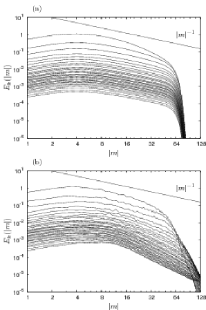
Figure 1: Cross-sectional spectra $E_{k}(|m|)$ of GM spectrum as the initial condition (upper) and of energy spectrum after about 35 hours (bottom) of Run I. Significant differences in the region $16<|m|<64$ indicates that GM spectrum is not statistically steady.

Since the GM spectrum was believed to be the universal oceanographic spectrum, the natural question to ask is whether the GM spectrum could be a steady state of our numerical wave model. We realize that such a guess may be far-fetched, but it is nevertheless appealing to check it. Therefore we are led to examine statistical stability of the GM spectrum. We assume that the steady state of the ocean can be characterized by an energy flux from pumping regions to damping regions in the wavenumber space. Therefore to achieve a truly steady state we need to model both pumping processes and damping processes. As explained above, in modeling the damping we use traditional hyper-viscosity approach in Eq. (15). As we will see below, the resulting spectrum depends upon the large-scale flows. Therefore, the only way to see whether the GM spectrum is close to being a steady state that is independent of the form of the pumping is to choose no pumping at all. Thus we are led towards modeling the system as a freely decaying system, i.e. without external forcing.

The GM spectrum with the cut-off in large horizontal and density wavenumbers is employed as the initial energy spectrum. The cut-off is introduced to avoid decreasing accuracy of the pseudo-spectral method. The initial phases of complex amplitude, $a(\bm{p})$, are given by uniformly distributed random numbers in $[0,2\pi)$.

Figure 1 shows the initial spectrum and the energy spectrum after about 35 hours in ocean time. If the GM spectrum were to be a universal steady state of our numerical model, it would change very little in this simulation. Instead, the density exponents rapidly change from $-1$ to $-2$ only after $1.5$ days. This spectral change occurs faster than dissipation effects with timescale estimated to be about 50 days at $|m|=32$. Therefore it appears that the GM spectrum is not a stable universal spectrum in the wavenumber region $16<|m|<64$ at least for this particular numerical experiment. The behavior of numerical experiment appears to contradict the arguments of McComas (1977); McComas and Müller (1981) based on induced diffusion approach that all energy spectra are rapidly relaxed to the GM spectrum, but is consistent with Winters and D’Asaro (1997).

IV.2 Run II and III

We certainly realize that our numerical model of Run I may not fully describe the ocean. Then we question what could be the nature of the statistical steady state of our wave model of stratified rotating turbulence. Here we model the pumping phenomenologically. We assume that waves are forced at horizontally and vertically large scales, i.e. small wavenumbers. In particular we choose the forced wavenumbers such that

$$|\bm{k}_{\mathrm{F}}|^{2}+|m_{\mathrm{F}}|^{2}\leq 6^{2}.$$ (28)

The forcing is modeled by fixing the amplitude of the forced wavenumbers to be constant in time. We also added an additional external dissipation $-D_{\omega}(\omega-N_{0})^{2}$ for $\omega>N_{0}$ in these runs to avoid violation of the hydrostatic balance. Detailed investigation of the non-hydrostatic effects is outside of the scope of present paper.

Since the energy flows in the wavenumber space strongly depend on the inertial frequencies $f$ Furuich et al. (2005), we performed Run II and III with differing values of the inertial frequencies $f$ (see Table 2). For Run II, the inertial frequency $f=0.25\times 10^{-4}$ rad/sec, while for Run III the value of the inertial frequency is $f=1\times 10^{-4}$ rad/sec. These inertial frequencies correspond to latitudes of 10 degrees and 45 degrees.

Note that there is a “critical” latitude where the frequency of the semidiurnal tide is equal to twice the inertial frequency. The principal difference between these two runs is that Run II is southwards of “critical” latitude in the northern hemisphere while Run III is northwards.

Our phenomenological forcing (28) corresponds to the band of frequencies greater than $4f$ for Run II and $\sqrt{2}f$ for Run III. These values are the result of the discreteness of the numerical grid. Certainly the forcing is not necessarily characteristic of the ocean and is purely phenomenological, and chosen for numerical simplicity and to allow easy interpretation.

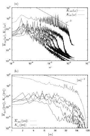
Figure 2: Integrated kinetic energy spectra $\overline{K}_{\mathrm{int}}(\omega)$ and $\overline{K}_{\mathrm{int}}(|m|)$, and cross-sectional energy spectra $K_{m}(\omega)$ and $K_{\omega}(|m|)$ of Run II. The kinetic energy spectra are obtained as functions of $\omega$ and $m$ from time and vertical series of the horizontal velocity $\bm{u}(\bm{x}_{0},\rho;t)$. The GM spectrum scales as $\omega^{-2}|m|^{-2}$ for large frequencies and density wavenumbers. The cross-sectional spectra that are functions of frequencies (left) are shown every eight curves for visibility. The cross-sectional spectra that are functions of vertical wavenumbers (right) are shown when $\omega=2,4,8,16,32\times 10^{-4}$rad/sec.

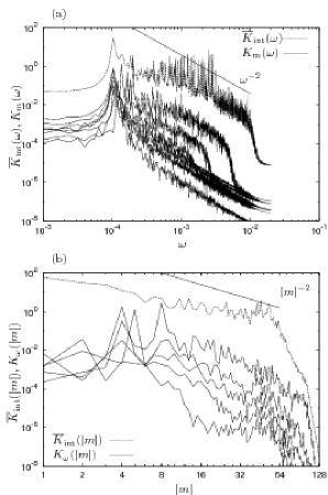
Figure 3: Integrated kinetic energy spectra, and cross-sectional energy spectra of Run III. See the caption of Fig. 2 for details.

The kinetic energy spectra as functions of $\omega$ and $m$ of Run II and III are shown in Figs. 2 and 3. Both frequency spectra (left in Figs. 2 and 3) have peaks at the inertial frequencies. This indicates that most energy accumulates in the near-inertial frequencies. The behavior is characteristic of the ocean. Indeed, these peaks correspond to the integrable singularity at the inertial frequency of the GM spectrum (22).

After about $10^{3}$ days from the initial time when all the wavenumbers have extremely small energy, the systems are still transient and the accumulation of energy in the near-inertial frequencies has not reached complete statistically steady states. Thus the timescale of the development of the accumulation is relatively large. Consequently one may conjecture that other processes, not present in our numerical model may affect the ocean at the large timescales. The most important of such processes which is not included in our simulations are the $\beta$ effects. Indeed, inclusion of $\beta$ effects would lead to existence of Rossby waves in our simulation, which may alter our results significantly. Other effects not present in our simulations, which can affect larger scales, may also alter the results. However, our subject is not to see how the energy spectra in the large-scale flows are formed but rather to investigate how the energy spectra in the inertial subrange are formed. For this subject, our numerical model is consistent with observationally-based intuition that wave-wave interactions is the predominant mechanism of forming the internal-wave spectrum in the inertial subrange.

The energy spectrum of Run II has only weak accumulation of energy in the near-inertial frequency. This could be qualitatively explained by the fact that all the forced wavenumbers have frequencies greater than $4f$ for Run II. Consequently, PSI is effective in transferring energy to frequencies around $2f$ and large vertical wavenumbers. Then PSI can no longer be effective in transferring energy towards the accumulation of energy in the near-inertial frequencies. Indeed, second PSI transfer would make the vertical wavenumber much larger and thus would move away from the accumulation. On the contrary, the energy spectrum of the Run III has moderate accumulation, stronger than that of Run II. This could be explained by the fact that the forced modes have frequencies greater than $\sqrt{2}f$. Then PSI can be effective in transferring energy from the wavenumbers that have frequency $2f$ to the accumulation whose frequencies are close to $f$ Furuich et al. (2005).

Since the forcing does not have just one frequency but several frequencies, the integrated spectra $\overline{K}_{\mathrm{int}}(\omega)$ have huge oscillations corresponding to the linear frequencies of the forced wavenumbers. Therefore, the power-law region of the frequencies, $10^{-4}\lesssim\omega\lesssim 10^{-2}$, are strongly contaminated by the forcing. However, the cross-sectional spectra with $|m|>6$ are not much affected by the forcing.

The vertical-wavenumber spectra (right in Figs. 2 and 3) appear to exhibit neither separable nor self-similar patterns. On the other hand, the integrated spectra do exhibit the self-similarity. The integrated spectra of the vertical wavenumbers are made mainly from the peaks at the near-inertial frequencies. Therefore, the cross-sectional spectra do not always have similarities to the integrated spectra.

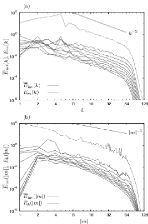
Figure 4: Integrated energy spectra $\overline{E}_{\mathrm{int}}(k)$ and $\overline{E}_{\mathrm{int}}(|m|)$, and cross-sectional energy spectra $E_{m}(k)$ and $E_{k}(|m|)$ of Run II. The GM spectrum scales as $k^{-2}|m|^{-1}$ for large horizontal and density wavenumbers. The cross-sectional spectra are shown every four curves for visibility.

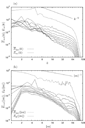
Figure 5: Integrated and cross-sectional spectra of Run III. See the caption of Fig. 4 for details.

It appears that it is advantageous to obtain $(k,m)$ spectra as well. The integrated energy spectra $\overline{E}_{\mathrm{int}}(k)$ and $\overline{E}_{\mathrm{int}}(|m|)$, and cross-sectional energy spectra $E_{m}(k)$ and $E_{k}(|m|)$ of Run II and Run III are shown in Fig. 4 and in Fig. 5, respectively. The figures indicate that the energy spectra as functions of $k$ and $m$ appear to be more separable than the kinetic energy spectra as functions of $\omega$ and $m$ in Run II and III.

Figure 6: Power-law exponents of each cross-sectional spectrum in Run II. left: $\alpha(|m|)$, which are the exponents of the cross-sectional energy spectra $E_{m}(k)$, right: $\beta(k)$, which are the exponents of the cross-sectional energy spectra $E_{k}(|m|)$. The error bars are obtained by fitting errors due to the least-square method. The exponents of the integrated spectra are also shown.

Figure 7: Power-law exponents of Run III. See the caption of Fig. 6 for details.

The integrated and cross-sectional spectra in Figs. 4 and 5 have power-law regions. The power-law exponents of the integrated and cross-sectional spectra are shown in Figs. 6 and 7. The power-law exponents of the cross-sectional spectra by the least-square fitting as

$$E_{m}(k)\propto k^{\alpha(|m|)}\quad\mathrm{in}\ k\in[8,40]$$

and

$$E_{k}(m)\propto|m|^{\beta(k)}\quad\mathrm{in}\ |m|\in[8,40].$$

The power-law exponents of the integrated spectra are also obtained as

$$\overline{E}_{\mathrm{int}}(k)\propto k^{\alpha_{\mathrm{int}}}$$

and

$$\overline{E}_{\mathrm{int}}(|m|)\propto|m|^{\beta_{\mathrm{int}}}$$

in the same wavenumber regions. In Run II the energy spectrum is close to double-power

$$E(k,m)\propto k^{-2}|m|^{-2.5}$$ (29)

in the large horizontal and density wavenumbers.

The exponents of the horizontal wavenumbers of both integrated and cross-sectional spectra, $\alpha_{\mathrm{int}}$ and $\alpha(m)$, roughly agree with the those of the GM spectrum, $-2$ of Eq. (26). This fact supports that the oceanic spectra of the internal waves can be explained by the wave-wave interactions. The integrated spectra are the sum of the cross-sectional spectra. The integrated spectra of the horizontal wavenumbers in the inertial subrange are not affected by the accumulation of energy around the horizontally longest waves.

Indeed, to obtain the integrated spectra as functions of horizontal wavenumbers, we use Eq. (17) and integrate over all $m$ value for each $k$ value. Thus, the integrals over vertical wavenumbers in large horizontal wavenumbers are unaffected by the strong presence of the near-inertial accumulation. Therefore the integrated spectra of $k$ in large horizontal wavenumbers well reflect the behavior of the spectra in the inertial subrange, and are immediately insensitive to the details of the accumulation of energy at small horizontal wavenumbers. Similar arguments can be applied to the integrated spectra of frequencies. Therefore, the integrated spectra of $\omega$ in high frequencies are determined by the behavior in the inertial subrange and are insensitive to the presence of the accumulation of energy at the near-inertial waves.

Consequently, the exponents of horizontal wavenumbers of both the integrated and cross-sectional spectra, $-2$, are characteristic in our numerical experiments, and is consistent with oceanographic observations.

On the other hand, to obtain the integrated spectra as functions of vertical wavenumbers, one should use Eq. (18) to integrate for each $m$ value over all $k$ values. Therefore, when integrating over $k$ values, the value of the integrals are always strongly affected by the accumulation of energy at small $k$ values. Therefore the exponents of the integrated spectra of $m$ are determined exclusive by the near-inertial accumulation, and are insensitive to the behavior in the inertial subrange. Consequently, the integrated spectra of $m$ are inconsistent in our simulations, and are in fact accumulation-dependent.

In actual fact, the integrated spectra as functions the vertical wavenumbers are less steep than the GM spectrum. Meanwhile, the cross-sectional spectra as functions the vertical wavenumbers in the inertial subrange are steeper than the GM spectrum. It comes from the fact that the exponents of the integrated spectra are a weighted mean of those of the cross-sectional spectra. In other words, $\beta_{\mathrm{int}}$ strongly depends on $\beta(1)$ and $\beta(2)$. Note that the horizontal wavenumbers $k=0$ corresponds to the inertial frequencies.

Figure 8: Power-law exponents of each cross-sectional spectrum of the kinetic energy in Run II. left: $A(|m|)$, which are the exponents of cross-sectional energy spectra $K_{m}(\omega)$ in Fig. 2, right: $B(\omega)$, which are the exponents of cross-sectional energy spectra $K_{\omega}(|m|)$ in Fig. 2.

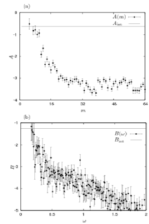
Figure 9: Power-law exponents of each cross-sectional spectrum of the kinetic energy in Run III. See the caption of Fig. 8 for details.

The energy spectrum does not have double-power laws in the large wavenumbers in Run III. It can be explained by contamination of the inertial subrange in the small horizontal wavenumbers and the large density wavenumbers, where the cross-sectional spectra do not show self-similarity in Fig. 5. It is curious that another double-power law appears in Run III in the small horizontal and density wavenumbers. Indeed, the spectrum at small wavenumbers can be approximated by

$$E(k,m)\propto k^{-2}|m|^{-2}.$$ (30)

As this power law does not appear in the inertial subrange, it has limited relevance to the scope of this paper.

Similar to the cross-sectional spectra in $(k,m)$ space, the spectral exponents in $(\omega,m)$ space could also be measured. The power-law exponents of the integrated and cross-sectional spectra of the kinetic energy in Figs. 2 and 3 are shown in Figs. 8 and 9. The least-square fittings are made in $\omega\in[10^{-4},10^{-3}]$rad/sec and $|m|\in[8,32]$ as $K_{m}(\omega)\propto\omega^{A(|m|)}$ and $K_{\omega}(m)\propto m^{B(|\omega|)}$. We cannot find any characteristic exponents in the figures. Therefore it appears that the spectral energy density of these runs is not separable in the $(\omega,m)$ space. This statement appears to be consistent with the fact that the cross-sectional spectra of the kinetic energy are neither self-similar nor separable.

To summarize, Runs II and III exhibit the accumulation of energy at the near-inertial waves. The formation mechanism of the near-inertial accumulation is consistent with the oceanographic PSI arguments. Furthermore, the cross-sectional spectra in Figs. 4 and 5 appear to be more separable than those in Figs. 2 and 3. It is supported by the fact that constant-exponent regions appear in the spectra in $(k,m)$ space (Figs. 6 and 7) but not in in the spectra in $(\omega,m)$ space (Figs. 8 and 9). Therefore, the spectrum appear to be more separable in $(k,m)$ space than in $(\omega,m)$ space in Run II and III. It also appears that the spectrum in the inertial subrange is sensitive to the details of the near-inertial accumulation. Most important, we reproduce the $-2$ exponent of the integrated spectra of the horizontal wavenumbers.

IV.3 Run IV

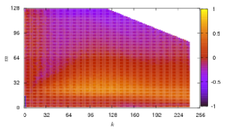
Figure 10: Relative difference between energy spectra after about $1.5$ days developed from the GM spectrum with and without energy in small horizontal wavenumbers $E_{\mathrm{d}}(k,|m|)$.

To further illustrate the influence of the accumulation around the horizontally longest waves, and to investigate the importance of the nonlocal interactions in the wavenumber space, we perform Run IV of Table 2. There we choose the initial condition same as the Run I but with no energy in $k<3$ and $|m|<16$. The energy spectrum after about $1.5$ days is denoted by $E_{\mathrm{nl}}(k,|m|)$. The energy spectrum developed from the GM spectrum in Run I that is shown in Fig. 1(right) is denoted by $E_{\mathrm{GM}}(k,|m|)$. Figure 10 shows the relative difference defined as

$$E_{\mathrm{d}}(k,|m|)=\frac{E_{\mathrm{nl}}(k,|m|)-E_{\mathrm{GM}}(k,|m|)}{E_{\mathrm{GM}}(k,|m|)}\,.$$ (31)

The wavenumbers different in the initial conditions appear as a black rectangle in bottom left in Fig. 10. If the nonlocal interactions with the accumulation of energy around the horizontally longest waves were not dominant, the relative difference in the inertial subrange in Fig. 10 would be small or slightly negative since the nonlinear interactions try to compensate the defect in the small wavenumbers. Instead, $E_{\mathrm{nl}}(k,|m|)$ has more than 20% energy in $10\lesssim|m|\lesssim 40$ and less energy transfer to the dissipation region in $|m|\gtrsim 80$. This suggests that the small wavenumbers in the accumulation of energy transfer energy from small density wavenumbers to large density wavenumbers in the inertial subrange. This scenario of the energy transfer to the large density wavenumbers is qualitatively consistent with the Induced Diffusion mechanism McComas (1977); McComas and Müller (1981).

IV.4 Run V

Run II and III have indicated that the external forcing at multiple frequencies does not produce smooth spectral energy density in the frequency space. We therefore are led to the question what would happen if the forced wavenumbers correspond to the single frequency. In Run V, the forced wavenumbers are modeled as M₂ tides and have an almost single frequency of $3f$. The single frequency forcing is significantly different from the band of forced frequencies in Run II and III. One of the reasons to choose $3f$ is to further confirm that PSI mechanism is effective. Indeed, PSI is dominant in transferring energy to small $k$ and large $m$ wavenumbers when the forced frequencies are greater than $2f$. Consequently, with $3f$ forcing PSI will create a second peak at $1.5f$. Although one could choose $2f$ as a forced frequency, we have chosen $3f$ in order to be able to distinguish the direct excitations that appear at $1.5f$ via PSI and the accumulation of energy at the near-inertial frequencies around $f$.

Fixing forced frequency to be $3f$, we still have a freedom of choosing forced wavenumbers. For simplicity, to implement the forcing numerically, the external forcing is added to 24 small wavenumbers whose frequencies are close to $3f$. Specifically, we keep the amplitudes of canonical variables, $a(\bm{p})$, to be constant in time for the following wavenumbers: $(\bm{k},m)=(\pm 1,0,\pm 2)$, $(0,\pm 1,\pm 2)$, $(\pm 1,\pm 1,\pm 3)$, $(\pm 2,0,\pm 4)$ and $(0,\pm 2,\pm 4)$.

Figure 11: Two-dimensional energy spectrum $E(k,|m|)$ of Run V. The contours are plotted every powers of ten from $10^{-10}$ to $1$. The straight line from the origin shows the wavenumbers $\omega=1.5f$. The inset is the enlargement of the area near the origin.

In Fig. 11 we show the two-dimensional energy spectrum close to a statistically steady state obtained in this simulation. We observe that there is a significant energy accumulation around $k\sim 1$, i.e. the horizontally longest waves. The wavenumbers that have $1\leq k\leq 2$ except the forced wavenumbers, which are considered as the accumulation of energy, account for approximately 60% of the total energy. Appearance of the accumulation in the near-inertial waves is consistent with oceanographic observations. It is also consistent with Runs II and III. This consistency in observing the accumulation of energy in the near-inertial waves is one of the main results of the present paper.

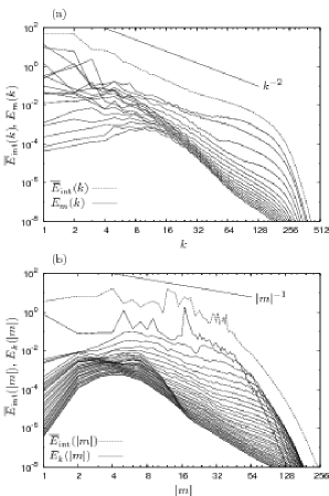
Figure 12: Integrated and cross-sectional spectra of Run V. See the caption of Fig. 4 for details.

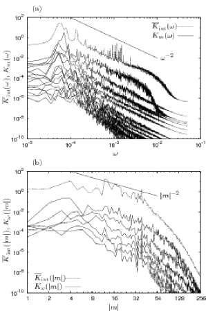
Figure 13: Integrated kinetic energy spectra, and cross-sectional energy spectra of Run V. The cross-sectional spectra that are functions of frequencies (left) are shown every eight curves for visibility. The cross-sectional spectra that are functions of vertical wavenumbers (right) are shown when $\omega=2.5,5,10,20,40\times 10^{-4}$rad/sec. See the caption of Fig. 2 for details.

Aside from the accumulation of energy around the horizontally longest waves, other excited wavenumbers appear around the line $\omega=1.5f$. The frequency is half of the frequency of the forced wavenumbers. This excitation can be qualitatively be explained by the PSI mechanism. Indeed, the excited wavenumbers whose frequencies are close to $1.5f$ make resonant triads with the forced wavenumbers via PSI. Furthermore, another excitation can be seen around $m\simeq 5$. The excitation can be interpreted as resonant interactions with the accumulation of energy due to the ES mechanism.

Figure 12 shows integrated spectra, $\overline{E}_{\mathrm{int}}(k)$ and $\overline{E}_{\mathrm{int}}(|m|)$, and cross-sectional spectra, $E_{m}(k)$ and $E_{k}(|m|)$, obtained from the two-dimensional energy spectrum shown in Fig. 11. The integrated spectra can be interpreted roughly to be

$$\overline{E}_{\mathrm{int}}(k)\propto k^{-1.98\pm 0.02}$$

and

$$\overline{E}_{\mathrm{int}}(|m|)\propto|m|^{-1.33\pm 0.31}.$$

The exponents are obtained with the least-square method in the intervals of $k\in[8,128]$ for $\overline{E}_{\mathrm{int}}(k)$ and that of $|m|\in[4,32]$ for $\overline{E}_{\mathrm{int}}(|m|)$. Note that the exponents are not too far from the large-wavenumber self-similar form of the GM spectrum. Indeed, the large wavenumber asymptotic form of the GM spectrum is given by Eq. (26).

We emphasize nevertheless that similarity of the integrated numerical spectrum as a function of vertical wavenumbers with Eq. (26) may be coincidental to some degree. The exponent of the integrated spectrum of the GM spectrum in large vertical wavenumbers is not $-1$ but $-2$. In addition, as apparent from Fig. 12, the spectrum in $(k,m)$ space is not separable. Moreover, as explained above, the exponent of the vertical wavenumbers is mostly determined by the accumulation of energy at small $k$. Consequently it is rather sensitive to the specifics of numerical experiments. On the other hand, the $k$ exponent is relatively insensitive to the accumulation and is determined by the inertial subrange. The behavior was also observed in Run II and III.

Figure 14: Power-law exponents of Run V. See the caption of Fig. 6 for details.

Figure 15: Power-law exponents of the kinetic energy in Run V. See the caption of Fig. 8 for details.

We also measure the kinetic energy spectrum in $(\omega,m)$ space. Figure 13 shows the results for Run V. It appears that some energy exists in the large frequencies greater than the buoyancy frequency. It comes mainly from the non-periodicity of the time series, and is called the Gibbs phenomenon.

Observe that the integrated spectrum of frequency is fitted by

$$\overline{E}_{\mathrm{int}}(\omega)\propto\omega^{-2.19\pm 0.11}.$$

over $\omega\in[10^{-4},10^{-3}]$. The asymptotic behavior is consistent with the GM spectrum and oceanographic observations. This is the main result of this paper. Also note that the vertical spectrum could be fitted by $|m|^{-1.12\pm 0.35}$ over $|m|\in[4,32]$.

Furthermore, one can interpret Fig. 13 as having three peaks in $\overline{E}_{\mathrm{int}}(\omega)$. The accumulation of energy makes the peak around the inertial frequency $f$ of this run, namely $5\times 10^{-5}$rad/sec. The second peak can be found around $7\times 10^{-5}$rad/sec which is the half of the frequency of the forced wavenumbers. Appearance of the excitation at half the forcing frequency is consistent with the PSI mechanism. The third peak is seen around $1.4\times 10^{-4}$rad/sec which is the frequency of the forced wavenumbers.

To illustrate the spectral details in the inertial subrange, we show the power-law exponents of each cross-sectional spectrum in Fig. 14, $\alpha(|m|)$ and $\beta(k)$. The exponents are obtained by fitting $E_{m}(k)\propto k^{\alpha(|m|)}$ in $k\in[16,128]$ and $E_{k}(m)\propto|m|^{\beta(k)}$ in $|m|\in[16,64]$. The exponents of the integrated spectra, $\alpha_{\mathrm{int}}=-1.98$ and $\beta_{\mathrm{int}}=-1.33$, are also shown in Fig. 14. The main point taken from the figure is that the integrated spectra have different exponents from the ones of the cross-sectional spectra in the inertial subrange. We observe that $\alpha$ varies between $-1$ and $-5$. Similarly, $\beta$ varies between $-1.5$ and $-3.5$.

Similar to Runs II and III, the exponent of the integrated spectrum of the horizontal wavenumbers is close to the GM spectrum. However, the cross-sectional spectra are steeper than the GM spectrum in the large horizontal and vertical wavenumbers considered as the inertial subrange. This can be explained by the fact that they are contaminated by direct excitations due to PSI and ES mechanisms. Apparently, the cross-sectional exponents are not constant. Therefore, the energy spectrum of the numerical simulation cannot be accurately fitted by double-power functions.

As the integrated and cross-sectional spectra of the GM spectrum have different exponents with respect to the vertical wavenumbers, the exponents of the integrated spectra are much different those of the cross-sectional spectra in the inertial subrange also in our simulations. This discrepancy is caused by the non-separability of the two-dimensional spectrum. The discrepancy in the vertical-wavenumber exponents is especially clear by the near-inertial accumulation. The integrated spectrum, $\overline{E}_{\mathrm{int}}(m)$, is established mainly by $E_{k=1,2}(m)$ i.e. the accumulation of energy. Therefore, the exponent of the integrated spectrum is determined exclusively by the exponents of the cross-sectional spectra in the small horizontal wavenumbers.

Figure 15 shows power-law exponents of each cross-sectional spectrum of the kinetic energy as functions of $\omega$ and $|m|$. The fits are made over $\omega\in[10^{-4},10^{-3}]$rad/sec or over $|m|\in[8,32]$. The exponents of the integrated spectra are also shown in the figure for reference. It is instructive to compare Figs. 14 and 15. It appears that the $(\omega,m)$ spectrum is more separable than the $(k,m)$ spectrum. Indeed, the exponent $\alpha$ of horizontal wavenumbers of the $(k,m)$ spectrum of Fig. 14 varies between $-1$ and $-5$, while the exponent $A$ of frequencies of the $(\omega,m)$ spectrum of Fig. 15 varies between $-1.5$ and $-4$. Furthermore, it appears that $A$ can loosely be represented as having the value of $A\simeq-2.7$. Similarly, apart from the small-wavenumber and low-frequency region, the exponent $\beta$ of vertical wavenumbers of the $(k,m)$ spectrum varies between $-2.5$ and $-3.5$, and the exponent $B$ of vertical wavenumbers of the $(\omega,m)$ spectrum can loosely be interpreted as having value around $-3.5$. However, the separability (1) can not be interpreted as being fully satisfied. Our observation of the spectrum of Run V being more separable in $(\omega,m)$ space than in $(k,m)$ space is consistent with observationally-based intuition. We again note that the exponents of the cross-sectional spectra are also far from those of the integrated spectra. This statement is true for both $(k,m)$ and $(\omega,m)$ spectra.

As explained above, the near-inertial accumulation appears only in the small horizontal wavenumbers and the small frequencies. Thus, the accumulation does not affect the integrated spectrum of $k$ in the large horizontal wavenumbers when the integration of the two-dimensional $(k,m)$ spectrum over $m$ to obtain the integrated spectrum is made. Similarly, the integrated spectrum of $\omega$ in high frequencies are not affected by the near-inertial accumulation. Then, we can argue that the integrated spectra of the horizontal wavenumbers and the frequencies are determined by the wavenumbers in the inertial subrange. Consequently these integrated spectra appear to be characteristic in our numerical runs. Therefore, the power-law exponents of the integrated spectra roughly corresponding to those of the observations including the GM spectrum reflects the nonlinear interactions of the internal-wave system.

To summarize, Run V is the largest and longest run that we have performed. The internal-wave field is forced by single frequency, small horizontal and vertical wavenumbers. Run V clearly demonstrates the energy accumulation around the horizontally longest waves. This run also shows that PSI mechanism is effective at creating a second peak at half the forced frequency. Furthermore, this run reproduce the integrated spectra, $k^{-2}$ spectrum and $\omega^{-2}$ spectrum. This is consistent with observations. This run also demonstrates that the spectrum in $(\omega,m)$ space is more separable than in $(k,m)$ space. It is also consistent with oceanic observations.

V Discussion

Stratified rotating turbulence is a complicated and fascinating subject. It has been a subject of intensive research in the last few decades. In particular various numerical simulations were performed. For example, Winters and D’Asaro (1997) numerically modeled stratified Navier–Stokes turbulence. They consider a depth dependent buoyancy frequency, and focus on a depth dependence of various physical quantities. Their simulation is done on a $32\times 256\times 129$ grid. They implemented realistic boundary conditions in the vertical directions and obtained the energy dissipation rates consistent with theories and observations. In contrast, our numerical simulations focus on spectral energy density.

More recent simulations were also performed. Laval et al. (2003) studied numerically stratified turbulence, and showed formation of pancake vortices and considerable amount of energy in the horizontally uniform vertical shear and vortical modes. Numerical simulations were also performed by Smith and Waleffe (2002) for rotating stratified turbulence and by Smith and Lee (2005) for rotating turbulence. These simulations demonstrate the tendency of energy to accumulate at the horizontally large-scale flows. They presented that the accumulation is caused mainly by resonant wave-wave interactions. They also obtained one-dimensional spectra similar to our integrated spectra.

In contrast to most of these simulations, our simulations are performed in periodic boxes in all three directions. Furthermore, we completely exclude vortices and horizontally uniform vertical shears. In addition, we use larger numerical grids, which are required in order to analyze the inner structures of the energy spectra in the inertial subrange. In addition, larger numerical grids are necessary to make the nonlocal interactions more pronounced in the simulations.

Certainly our reduced model constitutes a simplification of the ocean. One could argue that the horizontally uniform vertical shears excluded in our simulations might play an important role for the wavenumbers in the inertial subrange. Indeed, the horizontally uniform shear might strongly affect the spectra in the inertial subrange as the accumulation of energy at the horizontally longest waves does. Furthermore, the largest-scale motions also depend on other effects which are excluded from our simulation. In particular, we excluded variability of the inertial frequencies or $\beta$ effect, seasonal variability, and terrain properties. They may significantly affect the accumulation, providing mechanisms to diminish or build the accumulation. Consequently the waves in the inertial subrange will be affected.

As mentioned in Sec. I, anisotropic wave turbulence systems are often dominated by the nonlocal interactions. The oceanic internal waves are not an exception. Therefore it is important to study the effects of the nonlocal interactions in the wavenumber space.

The invariance under Galilean transformation is broken in the systems which have dominance of the nonlocal interactions. Indeed, Coriolis effect and presence of vertical stratification breaks the Galilean invariance of the internal waves. Consequently, one could argue that the dominance of the nonlocal interactions is caused by violation of Galilean invariance of the systems. In fact, in the systems where Galilean invariance is broken, the large-scale flows not only advect the small-scale flows but also actively exchange energy with them almost like an inertia force. It is in contrast with the typical behavior of the large-scale motions in Galilean-invariant systems. In Galilean-invariant systems the large-scale flows advect small-scale flows, as in the sweeping in Navier–Stokes turbulence.

VI Summary

In this work, we performed numerical modeling of the reduced wave-only stratified rotating turbulence in order to investigate the wave-wave interactions. In particular, we made a series of $5$ numerical runs with different initial conditions, grid sizes and forcing.

Run I is the freely decaying run with the GM spectrum employed as the initial condition. It has demonstrated that the GM spectrum is not a steady-state spectrum for our numerical model.

Runs II and III are forced–damped runs with different values of $f$. These runs consistently demonstrated the tendency of the energy to accumulate in the horizontally longest (i.e. near-inertial) waves. In these runs the level of the accumulation depends on the relation between the value of the inertial frequency $f$ and forced frequencies. The accumulation of energy in the near-inertial frequencies is characteristic of the oceans. The runs also demonstrated largely non-separable spectra. It also appears that the energy spectrum in $(k,m)$ space is more separable than in $(\omega,m)$ space. This is at odds with oceanic intuition. We also observed realistic $k^{-2}$ spectrum in Run II. Furthermore, the formation of the inertial peak is qualitatively consistent with a “named” nonlocal interaction, which is the Parametric Subharmonic Instability. It also appears that the integrated vertical-wavenumber spectrum is highly sensitive to the accumulation at the horizontally longest waves. Finally, the integrated frequency spectra cannot be fitted by power laws due to the forcing at multiple frequencies.

Run IV is the freely decaying run with the GM spectrum without the small wavenumbers as initial conditions. This run demonstrates that the internal-wave statistical properties are strongly affected by the nonlocal interactions with the small wavenumbers. In particular, removing the small wavenumbers from the initial condition produces a significantly different outcome. Thus, the energy transfer in the inertial subrange is qualitatively explained by the Induced Diffusion.

Run V also demonstrates that energy accumulates at the horizontally longest near-inertial waves. This is consistent with Runs II and III as well as the ocean. It also appears that the two-dimensional spectrum is more separable in $(\omega,m)$ space than in $(k,m)$ space. This is consistent with observationally-based intuition. Furthermore, the integrated frequency spectrum of Run V is given by $\omega^{-2}$, consistent with the ocean. Similarly, the integrated horizontal-wavenumber spectrum $k^{-2}$ is also consistent with the observations. However, the integrated vertical-wavenumber spectrum do not show the power-law exponent consistent with the observations. This could be explained by the fact that the integrated vertical-wavenumber spectrum is determined by the accumulation at the near-inertial waves. The near-inertial waves may be much affected by processes not considered in this manuscript.

In short, our numerical runs reproduce the following behavior:

• Energy tends to accumulate at the horizontally longest waves i.e. near-inertial waves

• To a lesser degree, some energy was observed in the small vertical wavenumbers.

• Spectra in the inertial subrange are not completely separable

• Realistic integrated horizontal $k^{-2}$ spectrum is observed

• Realistic integrated frequency $\omega^{-2}$ spectrum is observed

• The integrated vertical-wavenumber spectrum is determined exclusively by the near-inertial waves

• The spectrum in the inertial subrange is largely determined by the interactions with the near-inertial waves.

• The accumulation of energy of the near-inertial waves and the spectrum in the inertial subrange could qualitatively be described by “named” nonlocal interactions.

The stratified rotating turbulence governed by the Navier–Stokes equation and its relation with the ocean will of course be further researched and debated. Here we address the reduced wave-wave numerical model of stratified rotating turbulence with the hope that it could shed light on processes in oceans and its spectral energy density in particular. It appears that this reduced model reproduce key features of spectral energy density of oceanic internal waves. This supports observationally-based intuition that the spectral energy density of internal waves is described predominantly by the wave-wave interactions. The future will certainly bring many further exciting developments, and the synthesis of theoretical, observational and numerical results yet to be obtained.