Vibration-mediated resonant tunneling and shot noise through a molecular quantum dot

Abstract

Motivated by a recent experiment on nonlinear tunneling in a suspended Carbon nanotube connected to two normal electrodes [S. Sapmaz, et al., Phys. Rev. Lett. 96, 26801 (2006)], we investigate nonequilibrium vibration-mediated sequential tunneling through a molecular quantum dot with two electronic orbitals asymmetrically coupled to two electrodes and strongly interacting with an internal vibrational mode, which is itself weakly coupled to a dissipative phonon bath. For this purpose, we establish rate equations using a generic quantum Langevin equation approach. Based on these equations, we study in detail the current-voltage characteristics and zero-frequency shot noise, paying special attention to the advanced or postponed of the appearance of negative differential conductance and super-Poissonian current noise resulting from electron-phonon-coupling induced selective unidirectional cascades of single-electron transitions.

I Introduction

Recent progress in nanotechnology has facilitated the fabrication of single-electron tunneling devices using organic molecules. In turn, this has given rise to a large body of experimentaljPark ; hPark ; Zhitenev ; Yu ; Pasupathy ; LeRoy ; Sapmaz and theoreticalBose ; Alexandrov ; McCarthy ; Mitra ; Koch ; Koch1 ; Koch2 ; Zazunov ; Nowack ; Wegewijs ; Haupt work concerning phonon-mediated resonant tunneling through a quantum dot (QD) with strong coupling to an internal vibrational (phonon) mode (IVM). In particular, Carbon nanotubes (CNT) have recently become the focus of much research interest because electronic transport measurements show that they demonstrate perfect signatures of phonon-mediated tunneling, e.g. stepwise structures in the current-voltage characteristics having equal widths in voltage and gradual height reduction by the Franck-Condon (FC) factor.LeRoy ; Sapmaz

More interestingly, the experimental measurement of S. Sapmaz, et al.Sapmaz has revealed some more subtle transport features in a suspended CNT connected to two electrodes, particularly the appearance of a weak negative differential conductance (NDC) at the onset of each phonon step followed by a sudden suppression of current (a strong NDC) at a finite bias voltage after several steps for a long CNT sample. Theoretically, the reason for the weak NDC is quite clear in that it is ascribed to the combined effect of strong electron-phonon coupling (EPC) and low relaxation, i.e. an unequilibrated phonon (hot phonon), and strongly asymmetric tunnel-couplings to the left and right electrodes.Bose ; Koch2 ; Zazunov Furthermore, McCarthy, et al. have theoretically predicted the catastrophic current decrease, but their calculations are based on the presumption that the EPC is dependent on the applied bias voltage. It is appropriate to explore yet another explanation of the origin of the strong NDC without such an assumption.

Up to now, most theoretical works have focused on the case of a single level coupling to the phonon mode. However, it is believed that this catastrophic current decrease is intimately related to the tunneling processes involving two electronic energy levels. Nowack and Wegewijs have considered vibration-mediated tunneling through a two-level QD with asymmetric couplings to an IVM.Nowack Albeit their results display strong NDC through a competition between different FC tailored tunneling processes of the two levels, their calculations do not fully resolve the overall features of the experimental data in Ref. Sapmaz, . Following a suggestion by Hettler, et al.,Hettler that the interplay of strong Coulomb blockade and asymmetric tunnel-couplings of two levels to electrodes can lead to a strong NDC under certain conditions without EPC, we employ a model with two electronic orbitals having asymmetric couplings to the electrodes and with both strongly interacting with an IVM. We establish approximate rate equations at high temperature to describe resonant tunneling incorporating the unequilibrated phonon effect. Our results are in good qualitative agreement with the experiment data of Ref. Sapmaz, : in the weak bias voltage region where the first molecular orbital (MO) is dominant in electronic tunneling, the current shows the FC-type steplike structure and weak NDC at the onset of each step; while with increasing bias voltage the second MO becomes dominant in tunneling, inducing a sudden rapid reduction of current whether there is EPC or not. Furthermore, our studies predict that the onset of strong NDC as a function of voltage may differ from the value at which the second MO becomes active in resonant tunneling as described in Ref. Hettler, due to the unequilibrated phonon effect. We ascribe this to the EPC induced selective cascades of single-electron transitions between different charge states. In addition, we also analyze the current noise properties of this system. We find that the occurrence of weak and strong NDCs is accompanied by corresponding weak and strong enhancements of zero-frequency shot noise, respectively.

To emphasize the external-voltage-driven unequilibrated phonon effect in electronic tunneling in a CNT, we consider the IVM in our model coupled to an external dissipative environment (a phonon bath),Haupt and we incorporate the dissipation mechanism of the unequilibrated phonon into the ensuing rate equations on a microscopic basis. For extremely strong dissipation, our results naturally reduce to those of equilibrated phonon-mediated tunneling. Therefore, our rate equations provide a valuable theoretical framework for analysis of the mechanism by which finite phonon relaxation influences the electronic transport properties of CNT.

The outline of the paper is as follows. In Sec. II, we describe the model system that we study, and rewrite the model Hamiltonian in terms of an electron-phonon direct product (EPDP) state representation, which is suitable for the ensuing theoretical derivation. In Sec. III, we derive a set of rate equations using a generic quantum Langevin equation approach with a Markovian approximation, which facilitates investigation of uneqilibrated phonon and phonon dissipation effects on phonon-mediated electronic tunneling. In this section, we also derive the current formula using linear-response theory. In Sec. IV, we describe MacDonald’s formula for calculating zero-frequency shot noise by rewriting the ensuing rate equations in a number-resolved form. Then, we investigate in detail the vibration-mediated transport and shot noise properties of a molecular QD with two MOs in Sec. V. Finally, a brief summary is given in Sec. VI.

II Model Hamiltonian

In this paper, we consider a generic model for a molecular QD (in particular the suspended CNT) with two spinless levels, one as the highest-occupied MO (HOMO) $\varepsilon_{1}$ and the other as the lowest-unoccupied MO (LUMO) $\varepsilon_{2}$, coupled to two electrodes left (L) and right (R), and also linearly coupled to an IVM of the molecule having frequency $\omega_{0}$ with respective coupling strengths $\lambda_{1}$ and $\lambda_{2}$. We suppose that this single phonon mode is coupled to a dissipative environment represented as a set of independent harmonic oscillators (phonon-bath). The model Hamiltonian is

$$H=H_{leads}+H_{mol}+H_{B}+H_{I},$$ (1a)

with

$$H_{leads} = \sum_{\eta,{\bf k}}\varepsilon_{\eta{\bf k}}c_{\eta{\bf k}}^{\dagger}c_{\eta{\bf k}}^{\phantom{\dagger}},$$ (1b)

$$H_{mol} = \sum_{j=1,2}\varepsilon_{j}c_{j}^{\dagger}c_{j}^{\phantom{\dagger}}+Un_{1}n_{2}$$ (1d)

$$+\omega_{0}a^{\dagger}a+\sum_{j=1,2}\lambda_{j}c_{j}^{\dagger}c_{j}^{\phantom{\dagger}}(a^{\dagger}+a),$$

$$H_{B} = \sum_{p}\omega_{p}b_{p}^{\dagger}b_{p}^{\phantom{\dagger}},$$ (1e)

$$H_{I} = H_{T}+H_{vB},$$ (1f)

$$H_{T} = \sum_{\eta,{\bf k},j}(V_{\eta j}c_{\eta{\bf k}}^{\dagger}c_{j}+{\rm H.c.}),$$ (1g)

$$H_{vB} = (a^{\dagger}+a)\sum_{p}\kappa_{p}(b_{p}^{\dagger}+b_{p}),$$ (1h)

where $c_{\eta{\bf k}}^{\dagger}$ ($c_{\eta{\bf k}}$) is the creation (annihilation) operator of an electron with momentum ${\bf k}$, and energy $\varepsilon_{\eta{\bf k}}$ in lead $\eta$ ($\eta=L,R$), and $c_{j}^{\dagger}$ ($c_{j}$) is the corresponding operator for a spinless electron in the $j$th level of the QD ($j=1,2$). $U$ denotes interdot Coulomb interaction and $n_{j}=c_{j}^{\dagger}c_{j}^{\phantom{\dagger}}$ is the electron number operator in level $j$. $a^{\dagger}$ ($a$) and $b_{p}^{\dagger}$ ($b_{p}$) are phonon creation (annihilation) operators for the IVM and phonon-bath (energy quanta $\omega_{0}$, $\omega_{p}$), respectively. $\lambda_{j}$ represents the coupling constant between electron in dot $j$ and the IVM; $\kappa_{p}$ is the coupling strength between the IVM and phonon bath; $V_{\eta j}$ describes the tunnel-coupling between electron level $j$ and lead $\eta$. Here, we denote the density of states of the phonon bath with respect to frequency $\omega_{p}$ by $D(\omega_{p})$, and define the corresponding spectral density $J_{B}(\omega_{p})$ as

$$J_{B}(\omega_{p})=\kappa_{p}^{2}D(\omega_{p}).$$ (2)

In the literature, the following form of the spectral density is usually considered:Grabert

$$J_{B}(\omega_{p})=\kappa_{0}\omega_{p}^{\alpha}\theta(\omega_{p}),$$ (3)

in which $\theta(x)$ is the Heaviside step function. The bath is said to be Ohmic, sub-Ohmic, and super-Ohmic if $\alpha=1$, $\alpha<1$, and $\alpha>1$, respectively. We use units with $\hbar=k_{B}=e=1$ throughout the paper. In addition, it is worth noting that we do not consider the EPC-induced coupling between two MO’s in the Hamiltonian, Eq. (1d), because it is much weaker than the coupling of a single MO.

It is well-known that, in the strong electron-phonon interaction problem, it is very convenient to introduce a standard canonical transformationMahan to the Hamiltonian Eq. (1a), $\widetilde{H}=e^{S}He^{-S}$, with $S=(g_{1}n_{1}+g_{2}n_{2})(a^{\dagger}-a)$ ($g_{j}=\lambda_{j}/\omega_{0}$), which leads to a transformed Hamiltonian

$$\widetilde{H}_{mol} = \sum_{j}\widetilde{\varepsilon}_{j}c_{j}^{\dagger}c_{j}+\widetilde{U}n_{1}n_{2}+\omega_{0}a^{\dagger}a,$$ (4a)

$$\widetilde{H}_{I} = \widetilde{H}_{T}+\widetilde{H}_{vB},$$ (4b)

$$\widetilde{H}_{T} = \sum_{\eta,{\bf k},j}(V_{\eta j}c_{\eta{\bf k}}^{\dagger}c_{j}X_{j}+{\rm H.c.}),$$ (4c)

$$\widetilde{H}_{vB} = (a^{\dagger}+a-2\sum_{j}g_{j}n_{j})\sum_{p}\kappa_{p}(b_{p}^{\dagger}+b_{p}),$$ (4d)

with $$\widetilde{\varepsilon}_{j}=\varepsilon_{j}-\frac{\lambda_{j}^{2}}{\omega_{0}} \widetilde{U}=U-2\frac{\lambda_{1}\lambda_{2}}{\omega_{0}} X$$ and . Importantly, the -operator describes the phonon renormalization of dot-lead tunneling,

$$X_{j}=e^{g_{j}(a-a^{\dagger})}.$$ (4e)

Obviously, the model described by the above Hamiltonian Eq. (1a) involves a many-body problem with phonon generation and annihilation when an electron tunnels through the central region. Therefore, one can expand the electron states in the dot in terms of direct product states composed of single-electron states and $n$-phonon Fock states. In this two-level QD system, there are a total of four possible electronic states: (1) the two levels are both empty, $|0\rangle_{1}|0\rangle_{2}$, and its energy is zero; (2) the HOMO is singly occupied by an electron, $|1\rangle_{1}|0\rangle_{2}$, and its energy is $\varepsilon_{1}$; (3) the LUMO is singly occupied, $|0\rangle_{1}|1\rangle_{2}$, and its energy is $\varepsilon_{2}$; and (4) both orbitals are occupied, $|1\rangle_{1}|1\rangle_{2}$, and its energy is $\varepsilon_{1}+\varepsilon_{2}+U$. Of course, if the interdot Coulomb repulsion is assumed to be infinite, the double-occupation is prohibited. For the sake of convenience, we assign these Dirac bracket structures as dyadic kets (bras):dyadic namely, the slave-boson kets $e_{n}^{\dagger}=|0\rangle_{1}|0\rangle_{2}\otimes|n\rangle$, $d_{n}^{\dagger}=|1\rangle_{1}|1\rangle_{2}\otimes|n\rangle$, and pseudo-fermion kets $f_{1n}^{\dagger}=|1\rangle_{1}|0\rangle_{2}\otimes|n\rangle$, $f_{2n}^{\dagger}=|0\rangle_{1}|1\rangle_{2}\otimes|n\rangle$. Correspondingly, the electron operator $c_{j}$ and phonon operator $a$ can be written in terms of such ket-bra dyadics as:

$$c_{j} = \sum_{n=0}^{\infty}(e_{n}^{\dagger}f_{jn}+s_{\bar{j}}f_{\bar{j}n}^{\dagger}d_{n}),$$ (5)

$$a = \sum_{n=0}^{\infty}\sqrt{n+1}(e_{n}^{\dagger}e_{n+1}^{\phantom{\dagger}}+\sum_{j}f_{jn}^{\dagger}f_{jn+1}^{\phantom{\dagger}}+d_{n}^{\dagger}d_{n+1}^{\phantom{\dagger}}),$$ (6)

with $\bar{j}\neq j$ and $s_{1(2)}=\pm 1$ ($s_{2}=-1$ is due to anti-commutation relation of the Fermion operator). With these direct product states and dyadics considered as the basis, the density-matrix elements may be expressed as $\rho_{00}^{n}=\langle\hat{\rho}_{00}^{n}\rangle=\langle e_{n}^{\dagger}e_{n}^{\phantom{\dagger}}\rangle$, $\rho_{jj}^{n}=\langle\hat{\rho}_{jj}^{n}\rangle=\langle f_{jn}^{\dagger}f_{jn}^{{\phantom{\dagger}}}\rangle$, and $\rho_{dd}^{n}=\langle\hat{\rho}_{dd}^{n}\rangle=\langle d_{n}^{\dagger}d_{n}^{\phantom{\dagger}}\rangle$.

The transformed Hamiltonian can be replaced by the following form in the auxiliary particle representation:

$$\widetilde{H}_{mol} = \sum_{n}[n\omega_{0}e_{n}^{\dagger}e_{n}^{\phantom{\dagger}}+\sum_{j}(\widetilde{\varepsilon}_{j}+n\omega_{0})f_{jn}^{\dagger}f_{jn}^{\phantom{\dagger}}$$ (7b)

$$+(\widetilde{\varepsilon}_{1}+\widetilde{\varepsilon}_{2}+\widetilde{U}+n\omega_{0})d_{n}^{\dagger}d_{n}^{\phantom{\dagger}}],$$

$$\widetilde{H}_{T} = \sum_{\eta,{\bf k},j,n}[V_{\eta j}c_{\eta{\bf k}}^{\dagger}(e_{n}^{\dagger}f_{jn}+s_{\bar{j}}f_{\bar{j}n}^{\dagger}d_{n})X_{j}+{\rm H.c.}],$$ (7c)

$$\widetilde{H}_{vB} = \sum_{p}\kappa_{p}(b_{p}^{\dagger}+b_{-p})\left[\sum_{n}\sqrt{n+1}(e_{n}^{\dagger}e_{n+1}^{\phantom{\dagger}}\right.$$ (7g)

$$+\sum_{j}f_{jn}^{\dagger}f_{jn+1}^{\phantom{\dagger}}+d_{n}^{\dagger}d_{n+1}^{\phantom{\dagger}}+{\rm H.c.})$$

$$\left.-2\sum_{j,n}g_{j}(f_{jn}^{\dagger}f_{jn}^{\phantom{\dagger}}+d_{n}^{\dagger}d_{n}^{\phantom{\dagger}})\right].$$

Based on this transformed Hamiltonian, we derive a rate equation for description of the dynamics of the reduced density matrix of the combined electron and IVM system in the sequential tunneling regime.

III Quantum Langevin equation approach and rate equations

In this analysis, we employ a generic quantum Langevin equation approach,Schwinger ; Ackerhalt ; Cohen ; Milonni ; Gardiner ; Dong2 ; Dong3 starting from the Heisenberg equations of motion (EOMs) for the density-matrix operators $\hat{\rho}_{00}^{n}$, $\hat{\rho}_{jj}^{n}$ ($j=\{1,2\}$), and $\hat{\rho}_{dd}^{n}$:

$$i\dot{\hat{\rho}}_{00}^{n} = [e_{n}^{\dagger}e_{n}^{\phantom{\dagger}},\widetilde{H}]_{-}=\sum_{\eta,{\bf k},j,m}[V_{\eta j}c_{\eta{\bf k}}^{\dagger}e_{n}^{\dagger}f_{jm}X_{j,nm}$$ (8c)

$$-f_{jm}^{\dagger}e_{n}X_{j,nm}^{\dagger}c_{\eta{\bf k}}]+\sum_{p}\kappa_{p}(b_{p}^{\dagger}+b_{-p})$$

$$\times(\sqrt{n+1}e_{n}^{\dagger}e_{n+1}^{\phantom{\dagger}}+\sqrt{n}e_{n}^{\dagger}e_{n-1}^{\phantom{\dagger}}-{\rm H.c.}),$$

$$i\dot{\hat{\rho}}_{11}^{n} = [f_{1n}^{\dagger}f_{1n}^{\phantom{\dagger}},\widetilde{H}]_{-}=\sum_{\eta,{\bf k},m}[c_{\eta{\bf k}}^{\dagger}(V_{\eta 2}f_{1n}^{\dagger}d_{m}X_{2,nm}$$ (8g)

$$-V_{\eta 1}e_{m}^{\dagger}f_{1n}X_{1,mn})+(V_{\eta 1}f_{1n}^{\dagger}e_{m}X_{1,mn}^{\dagger}$$

$$-V_{\eta 2}d_{m}^{\dagger}f_{1n}X_{2,nm}^{\dagger})c_{\eta{\bf k}}]+\sum_{p}\kappa_{p}(b_{p}^{\dagger}+b_{-p})$$

$$\times(\sqrt{n+1}f_{1n}^{\dagger}f_{1n+1}^{\phantom{\dagger}}+\sqrt{n}f_{1n}^{\dagger}f_{1n-1}^{\phantom{\dagger}}-{\rm H.c.}),$$

$$i\dot{\hat{\rho}}_{22}^{n} = [f_{2n}^{\dagger}f_{2n}^{\phantom{\dagger}},\widetilde{H}]_{-}=\sum_{\eta,{\bf k},m}[-c_{\eta{\bf k}}^{\dagger}(V_{\eta 1}f_{2n}^{\dagger}d_{m}X_{1,nm}$$ (8l)

$$+V_{\eta 2}e_{m}^{\dagger}f_{2n}X_{2,mn})+(V_{\eta 1}f_{2n}^{\dagger}e_{m}X_{2,mn}^{\dagger}$$

$$+V_{\eta 2}d_{m}^{\dagger}f_{2n}X_{1,nm}^{\dagger})c_{\eta{\bf k}}]+\sum_{p}\kappa_{p}(b_{p}^{\dagger}+b_{-p})$$

$$\times(\sqrt{n+1}f_{2n}^{\dagger}f_{2n+1}^{\phantom{\dagger}}+\sqrt{n}f_{2n}^{\dagger}f_{2n-1}^{\phantom{\dagger}}-{\rm H.c.}),$$

$$i\dot{\hat{\rho}}_{dd}^{n} = [d_{n}^{\dagger}d_{n}^{\phantom{\dagger}},\widetilde{H}]_{-}=\sum_{\eta,{\bf k},m}[c_{\eta{\bf k}}^{\dagger}(V_{\eta 1}f_{2m}^{\dagger}d_{n}X_{1,mn}$$ (8q)

$$-V_{\eta 2}f_{1m}^{\dagger}d_{n}X_{2,mn})-(V_{\eta 1}d_{n}^{\dagger}f_{2m}X_{1,mn}^{\dagger}$$

$$-V_{\eta 2}d_{n}^{\dagger}f_{1m}X_{2,mn}^{\dagger})c_{\eta{\bf k}}]+\sum_{p}\kappa_{p}(b_{p}^{\dagger}+b_{-p})$$

$$\times(\sqrt{n+1}d_{n}^{\dagger}d_{n+1}^{\phantom{\dagger}}+\sqrt{n}d_{n}^{\dagger}d_{n-1}^{\phantom{\dagger}}-{\rm H.c.}),$$

where

$$X_{j,nm} = \langle n|X_{j}(t)|m\rangle,$$ (8r)

$$X_{j,nm}^{\dagger} = \langle m|X_{j}^{\dagger}(t)|n\rangle.$$ (8s)

These matrix elements can be calculated as:Mahan

$$X_{j,nm} = X_{j,nm}^{\dagger}$$ (9)

$$= \left\{\begin{array}[]{cc}e^{-g_{j}^{2}/2}g_{j}^{m-n}\sqrt{\frac{n!}{m!}}L_{n}^{m-n}(g_{j}^{2}),&n\leq m,\\ e^{-g_{j}^{2}/2}(-g_{j})^{n-m}\sqrt{\frac{m!}{n!}}L_{m}^{n-m}(g_{j}^{2}),&n>m,\end{array}\right.$$ (12)

where $L_{n}^{m}(x)$ is the generalized Laguerre polynomial. The rate equations are obtained by taking statistical expectation values of the EOMs, Eqs. (8c)-(8q), which clearly involve the statistical averaging of products of one reservoir (phonon-bath) variable and one device variable, such as ${\cal I}=\langle\sum_{{\bf k},\eta}V_{\eta 1}c_{\eta{\bf k}}^{\dagger}e_{n}^{\dagger}f_{1m}X_{1,nm}\rangle$ and ${\cal J}=\langle\sum_{p}\kappa_{p}(b_{p}^{\dagger}+b_{-p})\sqrt{n+1}(e_{n}^{\dagger}e_{n+1}^{\phantom{\dagger}}-{\rm H.c.})\rangle$.

To determine the products, ${\cal I}$ and ${\cal J}$, we proceed by deriving EOMs for the system, phonon-bath, and reservoir operators, $F_{1,nm}=e_{n}^{\dagger}f_{1m}^{\phantom{\dagger}}$, $\hat{\rho}_{00}^{n,n+1}=e_{n}^{\dagger}e_{n+1}^{\phantom{\dagger}}$, $b_{p}$, and $c_{\eta{\bf k}}$:

$$i\dot{F}_{1,nm} = [e_{n}^{\dagger}f_{1m},\widetilde{H}]_{-}=[\widetilde{\varepsilon}_{1}+(m-n)\omega_{0}]F_{1,nm}$$ (13b)

$$+[F_{1,nm},\widetilde{H}_{T}]_{-}+[F_{1,nm},\widetilde{H}_{vB}]_{-},$$

$$i\dot{\hat{\rho}}_{00}^{n,n+1} = [e_{n}^{\dagger}e_{n+1},\widetilde{H}]_{-}=\omega_{0}\hat{\rho}_{00}^{n,n+1}+[\hat{\rho}_{00}^{n,n+1},\widetilde{H}_{T}]_{-}$$ (13d)

$$+[\hat{\rho}_{00}^{n,n+1},\widetilde{H}_{vB}]_{-},$$

$$i\dot{b}_{p} = [b_{p},\widetilde{H}]_{-}=\omega_{p}b_{p}+[b_{p},\widetilde{H}_{vB}]_{-},$$ (13e)

$$i\dot{c}_{\eta{\bf k}} = [c_{\eta{\bf k}},\widetilde{H}]_{-}=\epsilon_{\eta{\bf k}}c_{\eta{\bf k}}+[c_{\eta{\bf k}},\widetilde{H}_{T}]_{-}.$$ (13f)

The EOM for $c_{\eta{\bf k}}^{\dagger}$ is easily obtained by Hermitian conjugation of the equations for $c_{\eta{\bf k}}$. Formally integrating these equations, (13b)-(13f), from initial time $0$ to $t$ we obtain

$$F_{1,nm}(t) = e^{-i[\widetilde{\varepsilon}_{1}+(m-n)\omega_{0}]t}F_{1,nm}(0)$$ (14c)

$$-i\int_{0}^{t}dt^{\prime}e^{-i[\widetilde{\varepsilon}_{1}+(m-n)\omega_{0}]\tau}[F_{1,nm}(t^{\prime}),\widetilde{H}_{T}(t^{\prime})]_{-}$$

$$-i\int_{0}^{t}dt^{\prime}e^{-i[\widetilde{\varepsilon}_{1}+(m-n)\omega_{0}]\tau}[F_{1,nm}(t^{\prime}),\widetilde{H}_{vB}(t^{\prime})]_{-},$$

$$\hat{\rho}_{00}^{n,n+1}(t) = e^{-i\omega_{0}t}\hat{\rho}_{00}^{n,n+1}(0)$$ (14g)

$$-i\int_{0}^{t}dt^{\prime}e^{-i\omega_{0}\tau}[\hat{\rho}_{00}^{n,n+1}(t^{\prime}),\widetilde{H}_{T}(t^{\prime})]_{-}$$

$$-i\int_{0}^{t}dt^{\prime}e^{-i\omega_{0}\tau}[\hat{\rho}_{00}^{n,n+1}(t^{\prime}),\widetilde{H}_{vB}(t^{\prime})]_{-},$$

$$b_{p}(t) = e^{-i\omega_{p}t}b_{p}(0)-i\int_{0}^{t}dt^{\prime}e^{-i\omega_{p}\tau}$$ (14j)

$$\times[b_{p}(t^{\prime}),\widetilde{H}_{vB}(t^{\prime})]_{-},$$

$$c_{\eta{\bf k}}(t) = e^{-i\epsilon_{\eta{\bf k}}t}c_{\eta{\bf k}}(0)-i\int_{0}^{t}dt^{\prime}e^{-i\epsilon_{\eta{\bf k}}\tau}$$ (14l)

$$\times[c_{\eta{\bf k}}(t^{\prime}),\widetilde{H}_{T}(t^{\prime})]_{-},$$

with $\tau=t-t^{\prime}$. In the absence of tunnel-coupling, $H_{I}\rightarrow 0$, we have

$$F_{1,nm}^{o}(t) = e^{-i[\widetilde{\varepsilon}_{1}+(m-n)\omega_{0}]\tau}F_{1,nm}^{o}(t^{\prime}),$$ (15a)

$$\hat{\rho}_{00,o}^{n,n+1}(t) = e^{-i\omega_{0}\tau}\hat{\rho}_{00,o}^{n,n+1}(t^{\prime}),$$ (15b)

$$b_{p}^{o}(t) = e^{-i\omega_{p}\tau}b_{p}^{o}(t^{\prime}),$$ (15c)

$$c_{\eta{\bf k}}^{o}(t) = e^{-i\epsilon_{\eta{\bf k}}\tau}c_{\eta{\bf k}}^{o}(t^{\prime}).$$ (15d)

A standard assumption in the derivation of a quantum Langevin equation is that the time scale of decay processes is much slower than that of free evolution, which is reasonable in the weak-tunneling approximation. This bespeaks a dichotomy of time-developments of the involved operators into a rapidly-varying (free) part and a slowly-varying (dissipative) part. Focusing attention on the slowly-varying decay processes, and noting that the infinitude of macroscopic bath variables barely senses reaction from weak interaction with the QD, it is appropriate to substitute the time-dependent decoupled reservoir, phonon-bath, and QD operators of Eqs. (15a)-(15d) into the integrals on the right of Eqs. (LABEL:solution1)-(14l). This yields approximate results for the reservoir operators as:Schwinger ; Ackerhalt ; Dong2 ; Dong3

$$c_{\eta{\bf k}}(t)=c_{\eta{\bf k}}^{o}(t)+c_{\eta{\bf k}}^{rT}(t),$$ (16a)

with

$$c_{\eta{\bf k}}^{rT}(t)=-i\int_{0}^{t}d\tau[c_{\eta{\bf k}}^{o}(t),\widetilde{H}_{T}^{o}(t^{\prime})]_{-},$$ (16b)

where $\widetilde{H}_{T(vB)}^{o}$ is composed of the operators in $\widetilde{H}_{T(vB)}$ which are replaced by their decoupled counterparts (interaction picture). In fact, this is just the operator formulation of linear response theory. Similarly, the approximate results for the QD and phonon-bath are also divided into two parts:

$$F_{1,nm}(t) = F_{1,nm}^{o}(t)+F_{1,nm}^{rT}(t)+F_{1,nm}^{rvB}(t)$$ (17a)

$$= F_{1,nm}^{o}(t)-i\int_{0}^{t}d\tau[F_{1,nm}^{o}(t),\widetilde{H}_{T}^{o}(t^{\prime})]_{-}$$ (17c)

$$-i\int_{0}^{t}d\tau[F_{1,nm}^{o}(t),\widetilde{H}_{vB}^{o}(t^{\prime})]_{-},$$

$$\hat{\rho}_{00}^{n,n+1}(t) = \hat{\rho}_{00,o}^{n,n+1}(t)+\hat{\rho}_{00,rT}^{n,n+1}(t)+\hat{\rho}_{00,rvB}^{n,n+1}(t)$$ (17d)

$$= \hat{\rho}_{00,o}^{n,n+1}(t)-i\int_{0}^{t}d\tau[\hat{\rho}_{00,o}^{n,n+1}(t),\widetilde{H}_{T}^{o}(t^{\prime})]_{-}$$ (17f)

$$-i\int_{0}^{t}d\tau[\hat{\rho}_{00,o}^{n,n+1}(t),\widetilde{H}_{vB}^{o}(t^{\prime})]_{-},$$

$$b_{p}(t) = b_{p}^{o}(t)+b_{p}^{rvB}(t)$$ (17g)

$$= b_{p}^{o}(t)-i\int_{0}^{t}d\tau[b_{p}^{o}(t),\widetilde{H}_{vB}^{o}(t^{\prime})]_{-}.$$ (17h)

Note that we use the super(sub)scripts $rT$ and $rvB$ denote the reactions from tunnel-coupling and environmental dissipation, respectively.

Employing the approximate solutions of Eqs. (16a), (16b) and (17c), we can evaluate ${\cal I}$ as

$${\cal I} = \sum_{\eta,{\bf k}}V_{\eta 1}\langle[c_{\eta{\bf k}}^{o\dagger}(t)+c_{\eta{\bf k}}^{r\dagger}(t)]$$ (19)

$$\times[F_{1,nm}^{o}(t)+F_{1,nm}^{r}(t)]X_{1,nm}\rangle$$

$$\simeq \sum_{\eta,{\bf k}}V_{\eta 1}\langle[c_{\eta{\bf k}}^{o\dagger}(t)F_{1,nm}^{r}(t)+c_{\eta{\bf k}}^{r\dagger}(t)F_{1,nm}^{o}(t)]X_{1,nm}\rangle.$$ (20)

The statistical averages involved here can be taken separately in regard to the electron ensembles of the reservoirs (many degrees of freedom) and in regard to the few degrees of freedom of the QD EPDP states. Accordingly, the statistical average of the product of one reservoir operator and one system operator factorizes in the averaging procedure. Therefore, the statistical average of $c_{\eta{\bf k}}^{o\dagger}(t)F_{1,nm}^{o}(t)$ vanishes. Moreover, in the sequential picture of resonant tunneling, the tunneling rates and current are proportional to second-order tunnel-coupling matrix elements. We thus neglect the term $c_{\eta{\bf k}}^{r\dagger}(t)F_{1,nm}^{r}(t)$ as it is proportional to the third-order tunnel-coupling matrix element, $O(V_{\eta j}^{3})$. The other interaction terms arise from tunneling reaction, and are of second-order of $V_{\eta j}$. After some lengthy but straightforward algebraic calculations, we obtain

$${\cal I} = -i\sum_{\eta}\Gamma_{\eta 1}\int d\epsilon\int_{0}^{t}d\tau e^{i(\epsilon-\widetilde{\varepsilon}_{1})\tau}\{f_{\eta}(\epsilon)\rho_{00}^{n}$$ (22b)

$$-[1-f_{\eta}(\epsilon)]\rho_{11}^{m}\}\bar{X}_{1,nm}^{\dagger}X_{1,nm}^{\phantom{\dagger}},$$

in which

$$\Gamma_{\eta j}=2\pi\varrho_{\eta}|V_{\eta j}|^{2}$$ (22c)

denotes the tunneling strength between the molecular orbital $$j \eta \varrho_{\eta} \eta f_{\eta}(\epsilon) \eta T$$ and lead ( is the density of states of lead ), is the Fermi-distribution function of lead with temperature , and

$$\bar{X}_{j,nm} = \langle n|X_{j}(t^{\prime})|m\rangle,$$ (22d)

$$\bar{X}_{j,nm}^{\dagger} = \langle m|X_{j}^{\dagger}(t^{\prime})|n\rangle.$$ (22e)

Considering $$a(t)=e^{-i\omega_{0}\tau}a(t^{\prime})$$, we have

$$\bar{X}_{j,nm} = e^{i(m-n)\omega_{0}\tau}X_{j,nm},$$ (22f)

$$\bar{X}_{j,nm}^{\dagger} = e^{-i(m-n)\omega_{0}\tau}X_{j,nm}.$$ (22g)

In the derivation of Eq. (22b), we assume that states with different phonon-numbers are completely decoherent, $\rho_{00(dd)}^{nm}=\rho_{00(dd)}^{n}\delta_{nm}$ and $\rho_{jj}^{nm}=\rho_{jj}^{n}\delta_{nm}$, owing to big energy difference between the two direct product states $|j,n\rangle$ and $|j,m\rangle$ if $n\neq m$. Moreover, a Markovian approximation will be adopted by making the replacement

$$\int_{-\infty}^{t}d\tau\Longrightarrow\int_{-\infty}^{\infty}d\tau,$$ (23)

in the statistical averaging, since we are interested in the long time scale behavior of these density matrix elements.

Furthermore, ${\cal J}$ can be evaluated using Eqs. (17f), (17h) with $b_{p}(t)=e^{-i\omega_{p}\tau}b_{p}(t^{\prime})$ as

$${\cal J} \simeq \sum_{p}\kappa_{p}\sqrt{n+1}\langle[(b_{p}^{o\dagger}(t)+b_{p}^{o}(t))$$ (26)

$$\times(\rho_{00,rvB}^{n,n+1}(t)-\rho_{00,rvB}^{n+1,n}(t))$$

$$+(b_{p}^{rvB\dagger}(t)+b_{p}^{rvB}(t))(\rho_{00,o}^{n,n+1}(t)-\rho_{00,o}^{n+1,n}(t))]\rangle$$

$$= -i\sum_{p}\kappa_{p}^{2}(n+1)\rho_{00}^{n}[(n_{B}(\omega_{p})+1)\delta(\omega_{p}+\omega_{0})$$ (30)

$$+n_{B}(\omega_{p})\delta(\omega_{p}-\omega_{0})]$$

$$+i\sum_{p}\kappa_{p}^{2}(n+1)\rho_{00}^{n+1}[n_{B}(\omega_{p})\delta(\omega_{p}+\omega_{0})$$

$$+(n_{B}(\omega_{p})+1)\delta(\omega_{p}-\omega_{0})],$$

in which $n_{B}(\omega_{p})=(e^{\omega_{p}/T}-1)^{-1}$ is the Bose-distribution function. With the assumption that the phonon-bath is composed of infinitely many harmonic oscillators having a wide and continuous spectral density, we can make the replacement, in the wide-band limit,

$$\sum_{p}\kappa_{p}^{2}(\cdots)\longrightarrow\int_{-\infty}^{\infty}d\omega_{p}\kappa_{p}^{2}D(\omega_{p})(\cdots),$$ (31)

yielding

$${\cal J}=-i\varpi_{p}n_{B}(\omega_{0})(n+1)\rho_{00}^{n}+i\varpi_{p}(n_{B}(\omega_{0})+1)(n+1)\rho_{00}^{n+1},$$ (32)

with $\varpi_{p}=\kappa_{0}\omega_{0}^{\alpha}$ being constant due to Eq. (3).

Following the same calculational scheme indicated above, we evaluated the other statistical expectation values involved in the EOMs, Eqs. (8c)-(8q). Finally, we obtained the following rate equations in terms of the direct product state representation of the density-matrix for the description of sequential tunneling through a molecular QD, accounting for the unequilibrated phonon effect and its modified tunneling rates, as well as IVM dissipation to the phonon environment:

$$\dot{\rho}_{00}^{n} = \sum_{m}\bigl{[}\Gamma_{1,nm}^{-}\rho_{11}^{m}+\Gamma_{2,nm}^{-}\rho_{22}^{m}-(\Gamma_{1,nm}^{+}+\Gamma_{2,nm}^{+})\rho_{00}^{n}\bigr{]}$$ (33b)

$$-(\varpi_{n}^{+}+\varpi_{n}^{-})\rho_{00}^{n}+\varpi_{n+1}^{-}\rho_{00}^{n+1}+\varpi_{n-1}^{+}\rho_{00}^{n-1},$$

$$\dot{\rho}_{11}^{n} = \sum_{m}\bigl{[}\Gamma_{1,mn}^{+}\rho_{00}^{m}-(\Gamma_{1,mn}^{-}+\widetilde{\Gamma}_{2,nm}^{+})\rho_{11}^{n}+\widetilde{\Gamma}_{2,nm}^{-}\rho_{dd}^{m}\bigr{]}$$ (33d)

$$-(\varpi_{n}^{+}+\varpi_{n}^{-})\rho_{11}^{n}+\varpi_{n+1}^{-}\rho_{11}^{n+1}+\varpi_{n-1}^{+}\rho_{11}^{n-1},$$

$$\dot{\rho}_{22}^{n} = \sum_{m}\bigl{[}\Gamma_{2,mn}^{+}\rho_{00}^{m}-(\Gamma_{2,mn}^{-}+\widetilde{\Gamma}_{1,nm}^{+})\rho_{22}^{n}+\widetilde{\Gamma}_{1,nm}^{-}\rho_{dd}^{m}\bigr{]}$$ (33f)

$$-(\varpi_{n}^{+}+\varpi_{n}^{-})\rho_{22}^{n}+\varpi_{n+1}^{-}\rho_{22}^{n+1}+\varpi_{n-1}^{+}\rho_{22}^{n-1},$$

$$\dot{\rho}_{dd}^{n} = \sum_{m}\bigl{[}\widetilde{\Gamma}_{2,mn}^{+}\rho_{11}^{m}+\widetilde{\Gamma}_{1,mn}^{+}\rho_{22}^{m}-(\widetilde{\Gamma}_{1,mn}^{-}+\widetilde{\Gamma}_{2,mn}^{-})\rho_{dd}^{n}\bigr{]}$$ (33h)

$$-(\varpi_{n}^{+}+\varpi_{n}^{-})\rho_{dd}^{n}+\varpi_{n+1}^{-}\rho_{dd}^{n+1}+\varpi_{n-1}^{+}\rho_{dd}^{n-1},$$

with the normalization relation $\sum_{n}(\rho_{00}^{n}+\rho_{11}^{n}+\rho_{22}^{n}+\rho_{dd}^{n})=1$. The electronic tunneling rates are defined as

$$\Gamma_{j,nm}^{+} = \sum_{\eta}\Gamma_{\eta j,nm}^{+}=\sum_{\eta}\Gamma_{\eta j}\gamma_{nm}^{j}f_{\eta}(\widetilde{\epsilon}_{j}+(m-n)\omega_{0}),$$ (34a)

$$\Gamma_{j,nm}^{-} = \sum_{\eta}\Gamma_{\eta j,nm}^{-}$$ (34c)

$$= \sum_{\eta}\Gamma_{\eta j}\gamma_{nm}^{j}[1-f_{\eta}(\widetilde{\epsilon}_{j}+(m-n)\omega_{0})],$$ (34d)

$$\widetilde{\Gamma}_{j,nm}^{+} = \sum_{\eta}\widetilde{\Gamma}_{\eta j,nm}^{+}$$ (34e)

$$= \sum_{\eta}\Gamma_{\eta j}\gamma_{nm}^{j}f_{\eta}(\widetilde{U}+\widetilde{\epsilon}_{j}+(m-n)\omega_{0}),$$ (34f)

$$\widetilde{\Gamma}_{j,nm}^{-} = \sum_{\eta}\widetilde{\Gamma}_{\eta j,nm}^{-}=\sum_{\eta}\Gamma_{\eta j}\gamma_{nm}^{j}$$ (34h)

$$\times[1-f_{\eta}(\widetilde{U}+\widetilde{\epsilon}_{j}+(m-n)\omega_{0})],$$

with the FC factor ($$p={\rm min}\{m,n\} q={\rm max}\{m,n\} m n$$ and , denoting the smaller and larger of the quantities and , respectively)

$$\gamma_{nm}^{j}=X_{j,nm}^{2}=e^{-g_{j}^{2}}g_{j}^{2|m-n|}\frac{p!}{q!}\bigl{[}L_{p}^{|m-n|}(g_{j}^{2})\bigr{]}^{2},$$ (34i)

describing the modification of tunnel-coupling due to phonon generation and emission during the electron tunneling processes. This FC factor is symmetric, $\gamma_{nm}^{j}=\gamma_{mn}^{j}$, and satisfies the sum rules $\sum_{n}\gamma_{nm}^{j}=\sum_{m}\gamma_{nm}^{j}=1$. Obviously, these rates have specific physical meanings: $\Gamma_{j,nm}^{+}$ ($\Gamma_{j,nm}^{-}$) describes the tunneling rate of an electron entering (leaving) level $j$ with null occupancy of level $\bar{j}$, together with the transition of vibrational quanta, $n\rightarrow m$ ($m\rightarrow n$); while $\widetilde{\Gamma}_{j,nm}^{+}$ ($\widetilde{\Gamma}_{j,nm}^{-}$) describes the tunneling rate of an electron entering (leaving) level $j$ with level $\bar{j}$ occupied, together with the corresponding transition of the IVM state.

The transition rates of phonon number states are

$$\varpi_{n}^{+} = \varpi_{p}n_{B}(\omega_{0})(n+1),$$ (35a)

$$\varpi_{n}^{-} = \varpi_{p}(n_{B}(\omega_{0})+1)n,$$ (35b)

which indicates that the state of the IVM changes from $n$ to $n+1$ ($n-1$) by absorbing (emitting) a phonon from (to) the phonon-bath without change of the electronic state. Note that $\varpi_{n}^{+}+\varpi_{n}^{-}$ defines the relaxation rate of the number state $n$ of the IVM due to dissipative coupling to the environment. Moreover, it should be pointed out that $\varpi_{p}=0$ denotes no dissipation of the IVM to the environment, signifying the maximal unequilibrated phonon effect in tunneling; while $\varpi_{p}=\infty$ denotes extremely strong dissipation of the IVM, so that it is always functions as an equilibrated state during each tunneling process, i.e., the excited phonon relaxes very quickly due to strong dissipation, before the next electronic tunneling event takes place. Obviously, strong dissipation, $\varpi_{p}=\infty$, forces the probability distributions on the right-hand side of Eqs. (33b)-(33h) to have the forms, $\rho_{00}^{n}=\rho_{00}P^{n}$, $\rho_{jj}^{n}=\rho_{jj}P^{n}$, and $\rho_{dd}^{n}=\rho_{dd}P^{n}$, with a thermal phonon distribution $P^{n}=e^{-n\omega_{0}/T}(1-e^{-\omega_{0}/T})$ (assuming the phonon bath to have the same temperature as the electrodes).

The tunneling current operator through the molecular QD is defined as the time rate of change of the charge density, $N_{\eta}=\sum_{{\bf k}}a_{\eta{\bf k}}^{\dagger}a_{\eta{\bf k}}^{{\phantom{\dagger}}}$, in lead $\eta$:

$$J_{\eta}=-\dot{N}_{\eta}=i[N_{\eta},\widetilde{H}]_{-}=i[N_{\eta},\widetilde{H}_{I}]_{-}.$$ (36)

Employing linear-response theory in the interaction picture,Mahan we have

$$I=\langle J_{L}\rangle=-i\int_{-\infty}^{t}dt^{\prime}\langle[J_{L}(t),\widetilde{H}_{I}^{o}(t^{\prime})]_{-}\rangle.$$ (37)

Following the same procedures indicated above,Dong2 ; Dong3 we obtain the current formula through the left lead in terms of the density matrix elements of direct product states as

$$I = \sum_{nm}\bigl{[}(\Gamma_{L1,nm}^{+}+\Gamma_{L2,nm}^{+})\rho_{00}^{n}+(\widetilde{\Gamma}_{L2,nm}^{+}-\Gamma_{L1,mn}^{-})\rho_{11}^{n}$$ (39)

$$+(\widetilde{\Gamma}_{L1,nm}^{+}-\Gamma_{L2,mn}^{-})\rho_{22}^{n}-(\widetilde{\Gamma}_{L1,mn}^{-}+\widetilde{\Gamma}_{L2,mn}^{-})\rho_{dd}^{n}\bigr{]}.$$

IV MacDonald’s formula for zero-frequency shot noise

In this section, we discuss the zero-frequency current noise of vibration-mediated sequential tunneling through a molecular QD involving an unequilibrated phonon. For this purpose, we employ MacDonald’s formula for shot noiseMacDonald based on a number-resolved version of the rate equations describing the number of completed tunneling events.Chen This can be derived straightforwardly from the established QREs, Eqs. (33b)–(33h). We introduce the two-terminal number-resolved density matrices $\rho_{jj}^{n(l,l^{\prime})}(t)$, representing the probability that the system is in the electronic state $|j\rangle$ ($j=\{0,1,2,d\}$) with $n$ vibrational quanta at time $t$ together with $l(l^{\prime})$ electrons occupying the left(right) lead due to tunneling events. Obviously, $\rho_{jj}^{n}(t)=\sum_{l,l^{\prime}}\rho_{jj}^{n(l,l^{\prime})}(t)$ and the resulting two-terminal number-resolved QREs for the case of an unequilibrated phonon are:

$$\dot{\rho}_{00}^{n(l,l^{\prime})} = \sum_{m}\bigl{[}\Gamma_{L1,nm}^{-}\rho_{11}^{m(l-1,l^{\prime})}+\Gamma_{L2,nm}^{-}\rho_{22}^{m(l-1,l^{\prime})}$$ (41d)

$$+\Gamma_{R1,nm}^{-}\rho_{11}^{m(l,l^{\prime}-1)}+\Gamma_{R2,nm}^{-}\rho_{22}^{m(l,l^{\prime}-1)}$$

$$-(\Gamma_{1,nm}^{+}+\Gamma_{2,nm}^{+})\rho_{00}^{n(l,l^{\prime})}\bigr{]}-(\varpi_{n}^{+}+\varpi_{n}^{-})\rho_{00}^{n(l,l^{\prime})}$$

$$+\varpi_{n+1}^{-}\rho_{00}^{n+1(l,l^{\prime})}+\varpi_{n-1}^{+}\rho_{00}^{n-1(l,l^{\prime})},$$

$$\dot{\rho}_{11}^{n(l,l^{\prime})} = \sum_{m}\bigl{[}\Gamma_{L1,mn}^{+}\rho_{00}^{m(l+1,l^{\prime})}+\Gamma_{R1,mn}^{+}\rho_{00}^{m(l,l^{\prime}+1)}$$ (41h)

$$-(\Gamma_{1,mn}^{-}+\widetilde{\Gamma}_{2,nm}^{+})\rho_{11}^{n(l,l^{\prime})}+\widetilde{\Gamma}_{L2,nm}^{-}\rho_{dd}^{m(l-1,l^{\prime})}$$

$$+\widetilde{\Gamma}_{R2,nm}^{-}\rho_{dd}^{m(l,l^{\prime}-1)}\bigr{]}-(\varpi_{n}^{+}+\varpi_{n}^{-})\rho_{11}^{n(l,l^{\prime})}$$

$$+\varpi_{n+1}^{-}\rho_{11}^{n+1(l,l^{\prime})}+\varpi_{n-1}^{+}\rho_{11}^{n-1(l,l^{\prime})},$$

$$\dot{\rho}_{22}^{n(l,l^{\prime})} = \sum_{m}\bigl{[}\Gamma_{L2,mn}^{+}\rho_{00}^{m(l+1,l^{\prime})}+\Gamma_{R2,mn}^{+}\rho_{00}^{m(l,l^{\prime}+1)}$$ (41l)

$$-(\Gamma_{2,mn}^{-}+\widetilde{\Gamma}_{1,nm}^{+})\rho_{22}^{n(l,l^{\prime})}+\widetilde{\Gamma}_{L1,nm}^{-}\rho_{dd}^{m(l-1,l^{\prime})}$$

$$+\widetilde{\Gamma}_{R1,nm}^{-}\rho_{dd}^{m(l,l^{\prime}-1)}\bigr{]}-(\varpi_{n}^{+}+\varpi_{n}^{-})\rho_{22}^{n(l,l^{\prime})}$$

$$+\varpi_{n+1}^{-}\rho_{22}^{n+1(l,l^{\prime})}+\varpi_{n-1}^{+}\rho_{22}^{n-1(l,l^{\prime})},$$

$$\dot{\rho}_{dd}^{n(l,l^{\prime})} = \sum_{m}\bigl{[}\widetilde{\Gamma}_{L2,mn}^{+}\rho_{11}^{m(l+1,l^{\prime})}+\widetilde{\Gamma}_{R2,mn}^{+}\rho_{11}^{m(l,l^{\prime}+1)}$$ (41p)

$$+\widetilde{\Gamma}_{L1,mn}^{+}\rho_{22}^{m(l+1,l^{\prime})}+\widetilde{\Gamma}_{R1,mn}^{+}\rho_{22}^{m(l,l^{\prime}+1)}$$

$$-(\widetilde{\Gamma}_{1,mn}^{-}+\widetilde{\Gamma}_{2,mn}^{-})\rho_{dd}^{n(l,l^{\prime})}\bigr{]}-(\varpi_{n}^{+}+\varpi_{n}^{-})\rho_{dd}^{n(l,l^{\prime})}$$

$$+\varpi_{n+1}^{-}\rho_{dd}^{n+1(l,l^{\prime})}+\varpi_{n-1}^{+}\rho_{dd}^{n-1(l,l^{\prime})}.$$

The current flowing through the system can be evaluated by the time rates of change of electron numbers in lead $\eta$ as

$$I_{\eta}=\dot{N}_{\eta}(t)=\frac{d}{dt}\sum_{l,l^{\prime}}l_{\eta}P^{(l,l^{\prime})}(t){\Big{|}}_{t\rightarrow\infty},$$ (42)

where

$$P^{(l,l^{\prime})}(t)=\sum_{n}[\rho_{00}^{n(l,l^{\prime})}(t)+\rho_{11}^{n(l,l^{\prime})}(t)+\rho_{22}^{n(l,l^{\prime})}(t)+\rho_{dd}^{n(l,l^{\prime})}(t)]$$ (43)

is the total probability of transferring $l(l^{\prime})$ electrons into the left(right) lead by time $t$ and $l_{\eta}=l(l^{\prime})$ with $\eta=L(R)$. It is readily verified that the current obtained from Eq. (42) by means of the number-resolved QREs, Eqs. (41d)–(41p), is exactly the same as that obtained from Eq. (LABEL:currentL). The zero-frequency shot noise with respect to lead $\eta$ is similarly defined in terms of $P^{(l,l^{\prime})}(t)$ as well:Dong3 ; MacDonald ; Chen

$$S_{\eta}(0)=2\frac{d}{dt}\left[\sum_{l,l^{\prime}}l_{\eta}^{2}P^{(l,l^{\prime})}(t)-(tI_{\eta})^{2}\right]{\Big{|}}_{t\rightarrow\infty}.$$ (44)

To evaluate $S_{\eta}(0)$, we define an auxiliary function $G_{jj}^{\eta n}(t)$ as

$$G_{jj}^{\eta n}(t)=\sum_{l,l^{\prime}}l_{\eta}\rho_{jj}^{n(l,l^{\prime})}(t),$$ (45)

whose equations of motion can be readily deduced employing the number-resolved QREs, Eqs (41d)–(41p), in matrix form: $\dot{\bm{G}}^{\eta}(t)={\cal M}_{\eta}{\bm{G}}^{\eta}(t)+{\cal G}_{\eta}{\bm{\rho}}(t)$ with ${\bm{G}}^{\eta}(t)=({\bm{G}}_{00}^{\eta},{\bm{G}}_{11}^{\eta},{\bm{G}}_{22}^{\eta},{\bm{G}}_{dd}^{\eta})^{T}$ and ${\bm{\rho}}(t)=({\bm{\rho}}_{00},{\bm{\rho}}_{11},{\bm{\rho}}_{22},{\bm{\rho}}_{dd})^{T}$ [here ${\bm{G}}_{jj}^{\eta}=(G_{jj}^{\eta 0},G_{jj}^{\eta 1},\cdots)^{T}$ and ${\bm{\rho}}_{jj}=(\rho_{jj}^{0},\rho_{jj}^{1},\cdots)^{T}$]. ${\cal M}_{\eta}$ and ${\cal G}_{\eta}$ can be obtained easily from Eqs. (41d)–(41p). Applying the Laplace transform to these equations yields

$${\bm{G}}^{\eta}(s)=(s{\bm{I}}-{\cal M}_{\eta})^{-1}{\cal G}_{\eta}{\bm{\rho}}(s),$$ (46)

where ${\bm{\rho}}(s)$ is readily obtained by applying the Laplace transform to its equations of motion with the initial condition ${\bm{\rho}}(0)={\bm{\rho}}_{st}$ [${\bm{\rho}}_{st}$ denotes the stationary solution of the QREs, Eqs (33b)–(33h)]. Due to the inherent long-time stability of the physical system under consideration, all real parts of nonzero poles of ${\bm{\rho}}(s)$ and ${\bm{G}}^{\eta}(s)$ are negative definite. Consequently, the divergent terms arising in the partial fraction expansions of ${\bm{\rho}}(s)$ and ${\bm{G}}^{\eta}(s)$ as $s\rightarrow 0$ entirely determine the large-$t$ behavior of the auxiliary functions, i.e. the zero-frequency shot noise, Eq. (44).

It is worth noting that (1) our two-terminal number-resolved QREs, Eqs. (41d)–(41p), facilitate evaluation of the bias-voltage dependent zero-frequency shot noise for arbitrary interdot hopping; (2) our calculations yield $S_{L}(0)=S_{R}(0)$.

V Results and discussion

We now proceed with numerical calculations of the current $I$ [Eq. (LABEL:currentL)], the zero-frequency current noise $S(0)$ and the Fano factor $F=S(0)/2I$ for the two-MO model in order to explain the particular experimental data in the current-voltage ($I$-$V$) characteristics recently reported for a suspended CNT.Sapmaz

For this purpose, we set the parameters in our calculations as: $\omega_{0}=1$ as the energy unit, $\Gamma_{R1}/\Gamma_{L1}=10^{3}$, $\Gamma_{L2}/\Gamma_{L1}=1$, $\Gamma_{R2}/\Gamma_{L1}=0.1$, $g_{1}=1$, and $\widetilde{\varepsilon}_{1}=0$, $\widetilde{\varepsilon}_{2}=4.0\omega_{0}$. For simplicity, we fix the energy of the ground MO to be zero and ignore the nonzero bias-voltage-induced energy shift of the MO, which can be achieved using gate voltage in the experiment. Different from Ref. Nowack, , we choose a large asymmetry in the tunneling rates of the first MO, $\Gamma_{R1}/\Gamma_{L1}=10^{3}$, and an intermediate electron-phonon coupling strength, $g_{1}$. In particular, numerical fits of the experimentally measured data for the $I$-$V$ curves show $g_{1}\simeq 1$ for long CNTs.Sapmaz These two parameters are believed to be necessary for the appearance of NDC in combination with the unequilibrated phonon condition, for the regime in which the ground MO is predominant in tunneling (this will be shown below).Zazunov Moreover, we also choose a large asymmetry in the tunneling rates of the second MO, $\Gamma_{R2}/\Gamma_{L2}=0.1$, which is responsible for the appearance of strong NDC when the excited MO is predominant in tunneling as pointed out in Ref. Hettler, . Furthermore, we examine the effect of EPC in the excited MO on the strong NDC.

In our calculations, $\varpi_{p}=0$ denotes no dissipation of the IVM to the environment, corresponding to the maximal uneqilibrated phonon effect in resonant tunneling; increasing dissipation strength, $\varpi_{p}>0$, describes the action of the dissipative environment as it begins to relax the excited IVM towards an equilibrium phonon state (in the limit $\varpi_{p}=\infty$). This parameter allows one to examine the continuous variation of the effect of the dissipative environment on the excited IVM, which is helpful in developing a deep understanding of the underlying properties of vibration-mediated resonant tunneling and its fluctuations in CNTs.Haupt Throughout the paper we set the temperature as $T=0.02\omega_{0}$ and assume that the bias voltage $V$ is applied symmetrically, $\mu_{L}=-\mu_{R}=V/2$.

V.1 Strong NDC in current-voltage characteristics

Figure 1 exhibits the calculated results without environmental dissipation, $\varpi_{p}=0$, for the $I$-$V$ characteristic and the occupation probability of the excited MO, $\rho_{22}$, in the case of strong Coulomb blockade $\widetilde{U}=\infty$. If the excited MO is weakly coupled to the IVM, for instance $g_{2}=0.01$ (solid lines) in Fig. 1, we find that (1) the ground MO plays a dominant role in tunneling if $V\leq 2\widetilde{\varepsilon}_{2}$($\simeq 8$); (2) a series of equally spaced steps in voltage appears in the $I$-$V$ curve demonstrating vibration-mediated transport behavior, associated with a gradually reduced step height due to the FC factor in this voltage range;Bose ; Alexandrov ; McCarthy ; Mitra ; Koch (3) a weak NDC and current peak occur at the onset of each step beginning from the second step, which are ascribed to the combination of asymmetric geometry, $\Gamma_{R1}/\Gamma_{L1}=10^{3}$,Zazunov and the unequilibrated phonon effect (this will be shown below); and (4) a strong NDC suddenly emerges when the excited MO becomes active in tunneling at $V=2\widetilde{\varepsilon}_{2}$, which helps to explain the experimental data [Fig. 3(a) in Ref. Sapmaz, ]. As pointed out previously by M. Hettler et al., who studied nonlinear transport through a molecular QD without IVM,Hettler this current decrease is a combined effect of strong Coulomb blockade and weak tunnel-coupling of the excited MO to the electrodes. It is for this reason that we selected $\Gamma_{R2}/\Gamma_{L1}=0.1$ in our numerical calculations. When the bias voltage increases to activate the excited MO, an electron can occupy this MO but does not easily tunnel out due to the weaker escape rate $\Gamma_{R2}$, as shown by the solid line in Fig. 1(b), thus blocking occupation of the ground MO because of the strong Coulomb repulsion. As a result, the tunneling current depends mainly on the contribution of the excited MO, leading to a suppression of current magnitude by about a factor $\Gamma_{R2}^{2}$. Relaxing either of these two conditions results in the elimination of the strong NDC. For example, the inset of Fig. 1 plots the corresponding results for the case without Coulomb interaction. Figure 2 shows the $I$-$V$ curve with increasing $\Gamma_{R2}$.

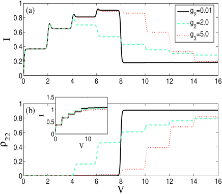
Figure 1: (a) Calculated current $I$, and (b) occupation probability $\rho_{22}$ as functions of bias voltage in the case of strong Coulomb blockade, $\widetilde{U}=\infty$, and unequilibrated phonon, $\varpi=0$ for $g_{2}=0.01$, $2.0$, and $5.0$. Inset: current $I$ vs. voltage $V$ in the case $\widetilde{U}=0$.

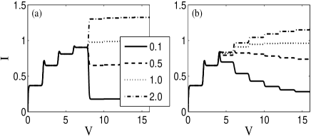
Figure 2: Current-voltage characteristics for several values of increasing tunneling rate $\Gamma_{R2}/\Gamma_{L1}$ with (a) $g_{2}=0.01$ and (b) $g_{2}=2.0$ in the case of strong Coulomb blockade, $\widetilde{U}=\infty$, and unequilibrated phonon, $\varpi=0$.

Interestingly, if the excited MO is also appreciably coupled to the IVM, a stepdown behavior with equally spaced width in voltage is superposed on the overall decrease of current, leading to a slowdown of the original rapid-reduction of current and more peaks of the NDC. More interestingly, an advancing and/or a postponing of the current decrease are observed, depending upon the relative strengths of the EPCs of the ground and excited MOs. Intuitively, this advancing and postponing can be ascribed to the corresponding behaviors of the occupation probability of the second MO in the presence of EPC, as shown in Fig. 1(b). In the following, we will offer a deeper theoretical explanation of these results.

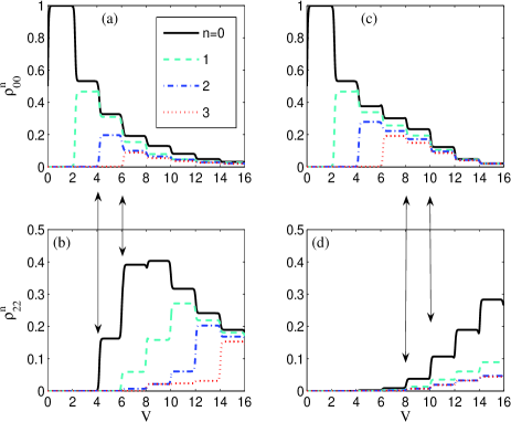
Figure 3: Electron-phonon joint occupation probabilities, $\rho_{00}^{n}$ (a,c) and $\rho_{22}^{n}$ (b,d), vs. bias voltage relevant to Fig. 1 parameters; for (a,b) $g_{2}=2.0$ and for (c,d) $g_{2}=5.0$.

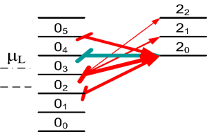
Figure 4: Allowed transitions for Fig. 3 (see text for details).

For illustrative purposes, it is helpful to examine bias voltage dependences of the electron-phonon joint occupation probabilities (EPJOPs), $\rho_{00}^{n}$ and $\rho_{22}^{n}$. We plot the calculated results in Fig. 3 for two cases with $g_{2}=2.0$ (a,b) and $g_{2}=5.0$ (c,d). It is unnecessary to plot the EPJOPs for the ground MO, $\rho_{11}^{n}$, because once an electron enters into the first MO from the left electrode, it will escape very rapidly to the right electrode due to the strongly asymmetric configuration, $\Gamma_{R1}/\Gamma_{L1}=10^{3}$ (We only consider $V>0$ in this paper). Therefore, all $\rho_{11}^{n}$ are nearly zero. In contrast to this, once an electron is injected into the second MO, it is effectively trapped in this MO due to the suppressed tunnel-out rate $\Gamma_{R2}/\Gamma_{L1}=0.1$ in the present model under investigation. With regard to this consideration, we first discuss the results for $g_{2}=2.0$. Fig. 3(a) clearly shows that the EPDP state $|0\rangle_{1}|0\rangle_{2}\otimes|n\rangle$ (for notational convenience, we use $0_{n}$ to denote this EPDP state and $2_{n}$ to represent $|0\rangle_{1}|1\rangle_{2}\otimes|n\rangle$ below) is occupied, and contributes to current when the Fermi energy of the left lead is equal to the energy of the corresponding direct product state, $\mu_{L}=n\omega_{0}$, as illustrated in the schematic energy diagram, Fig. 4. Opening a new channel will cause a decrease of the occupation probabilities of previous direct product states. Intuitively, one might think that the EPDP state $|0\rangle_{1}|1\rangle_{2}\otimes|0\rangle$($\equiv 2_{0}$) is unoccupied until the bias voltage increases to $V=2\widetilde{\varepsilon}_{2}=8.0\omega_{0}$. From Fig. 3(b), however we (surprisingly) observe that the EPDP state $2_{0}$ is actually becoming occupied even at $V=4.0\omega_{0}$, which is half of the conventional resonant tunneling value. Moreover, the EPDP states $2_{1}$ and $2_{2}$ are both becoming occupied starting at $V=6.0\omega_{0}$, albeit their corresponding resonant values should traditionally be $V=10.0\omega_{0}$ and $12.0\omega_{0}$ respectively. In addition, differing from the voltage dependence features of $\rho_{00}^{n}$, the opening of new channels involving the excited MO does not cause a reduction of the occupation probabilities of previous channels. These peculiar properties can be understood qualitatively in terms of phonon-induced cascaded single-electron transitions as illustrated in Fig. 4. As pointed out by M.R. Wegewijs, et al., arbitrarily high vibrational excitations can in principle be accessed via cascades of single-electron tunneling processes driven by a finite bias voltage, since transitions between the EPDP states is related to the variation of electronic energy and the change of phonon-number states. For instance, if the Fermi energy of the left lead is located between the EPDP states $0_{2}$ and $0_{3}$ with increasing bias voltage, i.e., $4.0\omega_{0}<V<6.0\omega_{0}$, the EPDP state $0_{2}$ becomes occupied as shown in Fig. 3(a). Moreover, the single-electron transition, $0_{2}\rightarrow 2_{0}$, indicated by the arrow in Fig. 4 is also permitted because the bias voltage $V=4.0\omega_{0}$ provides sufficient energy to activate this transition, $\widetilde{\varepsilon}_{2}+(0-2)\omega_{0}=2.0\omega_{0}$. As a result, albeit the Fermi energy of the left lead is not aligned with the energy $\widetilde{\varepsilon}_{2}=4.0\omega_{0}$ of the EPDP state $2_{0}$, this state also becomes occupied [Fig. 3(b)], which precedes the conventional resonance value $V=8.0\omega_{0}$. Likewise, when the bias voltage increases to $V>6.0\omega_{0}$, the EPDP state $0_{3}$ becomes occupied, and concomitantly, the transitions $0_{3}\rightarrow 2_{0}$, $0_{3}\rightarrow 2_{1}$, $0_{3}\rightarrow 2_{2}$, and even $0_{1}\rightarrow 2_{0}$ are also permitted with differing transition rates depending on the FC factors (denoted by the different widths of the arrows in Fig. 4) via the cascade transition mechanism. Therefore, we observe from Fig. 3(b) that the states $2_{1}$ and $2_{2}$ both become occupied starting at $V=6.0\omega_{0}$. In contrast to the situation in Ref. Nowack, , the back-transition $2_{n}\rightarrow 0_{m}$ is prohibited in the present model due to the above-mentioned trapping effect of the excited MO (stemming from the suppressed escape rate $\Gamma_{R2}$). Consequently, we find an accumulated increase of occupation probabilities of the EPDP states with low vibrational excitations up to a threshold value of bias voltage, in which a considerably large number of channels are stimulated and become active. In sum, the EPC-induced unidirectional cascaded transitions are responsible for the advanced appearance of NDC at lower bias voltages than one might otherwise expect.

We now turn to examine the mechanism of the postponed appearance of NDC in the case of $g_{2}=5.0\gg g_{1}$. Figures 3(c) and (d) show that the occupation probabilities of $\rho_{00}^{n}$ have a similar bias voltage dependence to that of the case of $g_{2}=2.0\sim g_{1}$, but the situation is considerably different for $\rho_{22}^{n}$: obviously, $\rho_{22}^{0}$ is nearly zero until the bias voltage increases up to $10.0\omega_{0}$, which is even higher than the resonance value, $V=2\widetilde{\varepsilon}_{2}=8.0\omega_{0}$. Therefore, it is interesting to explore why the EPC-induced cascade mechanism of single-electron transitions does not work in this situation. Albeit the cascade mechanism for the transition, e.g. $0_{2}\rightarrow 2_{0}$, satisfies the usual resonance condition from the energetic point of view, the actual occurrence of this transition still depends on the relevant transition rate determined by the corresponding FC factor, $\gamma_{02}^{2}$. In Fig. 5, we show the FC factors $\gamma_{nm}^{2}$ from $n,m=0$ to $10$ for $g_{2}=2.0$ and $5.0$, respectively. Clearly, a nearly vanishing FC factor $\gamma_{02}^{2}$ occurs if $g_{2}=5.0$. The strong EPC strength even blocks the conventional resonant transition $0_{4}\rightarrow 2_{0}$. Only when a large number of transitions are opened by a sufficiently high bias voltage (e.g. $V=10.0\omega_{0}$ here), can a significant occupation of $\rho_{22}$ be accumulated, thus leading to the current decrease.

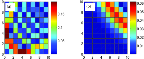
Figure 5: The FC factors, $\gamma_{nm}^{2}$ ($n,m=0$–$10$), for (a) $g_{2}=2.0$ and (b) $g_{2}=5.0$.

We now further examine the disappearance of NDC shown in Fig. 2(b). With gradual relaxation of the trapping effect of the excited MO (increasing $\Gamma_{R2}$), the unidirectional cascaded transitions becomes bidirectional, i.e., not only can the transitions $0_{n}\rightarrow 2_{m}$ occur, but also $2_{n}\rightarrow 0_{m}$ occurs as well, provided that the energy conservation condition is satisfied and the FC factor permits. Therefore, the inverse transition, $2_{0}\rightarrow 0_{2}$, reduces the occupation of the state $2_{0}$ (not shown here), and finally reduces the NDC.

V.2 Effects of dissipation to environment and super-Poissonian current noise

We now discuss the effects of environmental dissipation on the current and zero-frequency shot noise. Figures 6 and 7 exhibit the dissipation dependences of the current $I$ and Fano factor $F=S(0)/2I$ as functions of bias voltage for systems having $g_{2}=0.01$ and $2.0$, respectively.

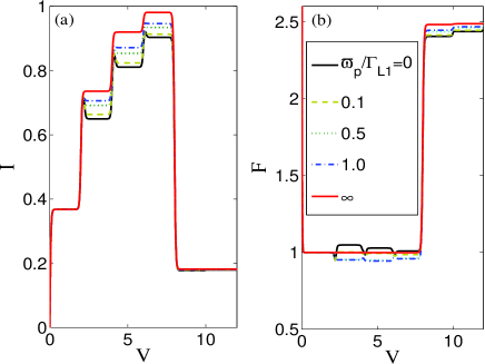
Figure 6: Calculated current, $I$ (a) and Fano factor, $F=S(0)/2I$ (b) vs. bias voltage for the case of $g_{2}=0.01$ and various environmental dissipation rates $\varpi_{p}$. Other parameters are the same as in Fig. 1.

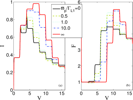
Figure 7: The same figure as Fig. 6 except that $g_{2}=2.0$.

In the region where the ground MO is dominant in tunneling, it is clearly observed that the weak NDC becomes ever weaker with a gradually increasing dissipation rate $\varpi$. The $I$-$V$ characteristic finally exhibits only positive differential conductance at $\varpi=\infty$, i.e., the equilibrated phonon condition. Therefore, one can conclude that the observation of weak NDC in the recent transport measurements clearly indicates that the external voltage-driven unequilibrated phonon effect in a suspended CNT plays an essential role in determining its underlying transport properties.Sapmaz Moreover, it is also clear that, due to the unequilibrated phonon effect, the current noise shows a weak super-Poissonian characteristic ($F>1$) associated closely with the appearance of NDC. Furthermore, the environmental dissipation suppresses the Fano factor and for certain values of the dissipation rate, $\varpi$, the shot noise shows weak sub-Poissonian behavior ($F<1$), but it becomes Poissonian ($F=1$) at the equilibrated phonon condition. This is just the traditional value of the Fano factor, $F=(\Gamma_{L1}^{2}+\Gamma_{R1}^{2})/(\Gamma_{L1}+\Gamma_{R1})^{2}$, for the extremely asymmetrical configuration $\Gamma_{R1}/\Gamma_{L1}=10^{3}$.

From Figs. 6 and 7, we find strong super-Poissonian shot noise as a companion to the strong NDC when the second MO starts to contribute to the current, irrespective of the environmental dissipation. When the second MO is also coupled to the IVM, the environmental dissipation strongly influences the current and noise as shown in Fig. 7. In particular, the threshold value of bias voltage for strong NDC and strong enhancement of shot noise is exactly the traditional resonant tunneling value of the second MO.

VI Conclusions

In summary, we have fully analyzed the external-bias-voltage-driven nonequilibrated phonon effect on nonlinear tunneling through a suspended CNT in the sequential tunneling regime. In order to qualitatively address the recent experimental results, we have modeled the CNT as a molecular QD having two electronic MOs with asymmetric tunnel-coupling rates to the left and right electrodes and strong interaction with an IVM. To study the role of dissipation of unequilibrated phonons, we have assumed further that the molecular IVM is also weakly coupled to a phonon bath “environment”. To carry out this analysis, we established generic rate equations in terms of the EPDP state and auxiliary-particle representation for the description of vibration-mediated resonant tunneling employing a microscopic quantum Langevin equation approach in the limit of weak tunneling and weak dissipation.

Employing the ensuing rate equations derived here, we systematically analyzed vibration-mediated resonant tunneling in the present model, obtaining the $I$-$V$ characteristics, zero-frequency current noise, and the effects of environmental dissipation on the role of the unequilibrated phonons. Our numerical analysis shows that in the voltage region where the ground orbital is dominant in tunneling, the combined effect of unequilibrated phonons and asymmetric tunnel-couplings is responsible for weak peaklike structures in the $I$-$V$ curve at the onset of each phonon step with a weak NDC and correspondingly weak super-Poissonian noise. Furthermore we found that this peaklike structure could be gradually diminished by environmental dissipation of the uneqilibrated IVM and become completely devoid of NDC at the equilibrated phonon condition. Accordingly, the usual current noise for an asymmetric single-electron tunneling device is predicted at the equilibrated phonon condition, $F=1$; however, for a finite dissipation rate suppressed noise, $F<1$, may be observed under certain conditions.

More interestingly, we have also discussed the transport properties in detail in the second-orbital dominated region. We found that the interplay of strong Coulomb interaction between the two MOs and strong asymmetry of tunnel-coupling leads to very strong NDC and a correspondingly strongly enhanced shot noise, irrespective of the EPC. However, the bias voltage value for the onset of NDC and super-Poissonian shot noise is intimately dependent on the EPC strength of the second MO, i.e., this voltage value can be smaller or larger than the traditional resonant tunneling value for the second MO. Our discussion concluded that this feature stems from the EPC-induced selective cascades of single-electron transitions with FC-factor-modified rates in a unidirectional way due to the asymmetric tunnel-coupling. Environmental dissipation forces this value to tend to the traditional resonance point.

References

• (1) H. Park, J. Park, A. Lim, E. Anderson, A. Allvisatos, and P. McEuen, Nature 407, 57 (2000).
• (2) J. Park, A.N. Pasupathy, J.I. Goldsmith, C. Chang, Y. Yaish, J.R. Petta, M. Rinkoski, J.P. Sethna, H. Abruna, P.L. McEuen, and D.C. Ralph, Nature 417, 722 (2002).
• (3) N.B. Zhitenev, H. Meng, and Z. Bao, Phys. Rev. Lett. 88, 226801 (2002).
• (4) L.H. Yu, Z.K. Keane, J.W. Ciszek, L. Cheng, M.P. Stewart, J.M. Tour, and D. Natelson, Phys. Rev. Lett. 93, 266802 (2004); L.H. Yu and D. Natelson, Nano Lett. 4, 79 (2004).
• (5) A.N. Pasupathy, J. Park, C. Chang, A.V. Soldatov, S. Lebedkin, R.C. Bialczak, J.E. Grose, L.A.K. Donev, J.P. Sethna, D.C. Ralph, and P.L. McEuen, Nano Lett. 5, 203 (2005).
• (6) B.J. LeRoy, S.G. Lemay, J. Kong, and C. Dekker, Nature 432, 371 (2004); B.J. LeRoy, J. Kong, V.K. Pahilwani, C. Dekker, and S.G. Lemay, Phys. Rev. B 72, 75413 (2005).
• (7) S. Sapmaz, P. Jarillo-Herrero, Ya.M. Blanter, C. Dekker, and H.S.J. van der Zant, Phys. Rev. Lett. 96, 26801 (2006); S. Sapmaz, P. Jarillo-Herrero, Ya.M. Blanter, and H.S.J. van der Zant, New J. Phys. 7, 243 (2005).
• (8) D. Bose and H. Schoeller, Europhys. Lett. 54, 668 (2001).
• (9) A.S. Alexandrov and A.M. Bratkovsky, Phys. Rev. B 67, 235312 (2003).
• (10) K.D. McCarthy, N. Prokof’ev, and M.T. Tuominen, Phys. Rev. B 67, 245415 (2003).
• (11) A. Mitra, I. Aleiner, and A.J. Millis, Phys. Rev. B 69, 245302 (2004).
• (12) J. Koch and F. von Oppen, Phys. Rev. Lett. 94, 206804 (2005).
• (13) J. Koch, M.E. Raikh, and F. von Oppen, Phys. Rev. Lett. 95, 56801 (2005).
• (14) J. Koch and F. von Oppen, Phys. Rev. B 72, 113308 (2005).
• (15) A. Zazunov, D. Feinberg, and T. Martin, Phys. Rev. B 73, 115405 (2006).
• (16) K.C. Nowack and M.R. Wegewijs, cond-mat/0506552 (2005)
• (17) M.R. Wegewijs, K.C. Nowack, New J. Phys. 7, 239 (2005).
• (18) F. Haupt, F. Cavaliere, R. Fazio, and M. Sassetti, Phys. Rev. B 74, 205328 (2006).
• (19) M. Hettler, H. Schoeller, and W. Wenzel, EuroPhys. Lett. 57, 571 (2002).
• (20) H. Grabert, P. Schramn, and G. Ingold, Phys. Rep. 3, 115 (1988).
• (21) G.D. Mahan, Many-Particle Physics. (Third edition, Kluwer Academic/Plenum Publisher, New York, 2000).
• (22) The dyadic operators are pseudo-operators defined as: ${\hat{a}}^{\dagger}=|A\rangle$ and $\hat{a}=\langle A|$ ($|A\rangle$ is a quantum state). The combination of dyadic operators gives a real operator ${\hat{a}}^{\dagger}b=|A\rangle\langle B|$ describing the transition from the state B to the state A, or the inner product $\hat{b}{\hat{a}}^{\dagger}=\langle B|A\rangle$ between the states $|A\rangle$ and $|B\rangle$.
• (23) J. Schwinger, J. Math Phys. 2, 417 (1961).
• (24) J.R. Ackerhalt and J.H. Eberly, Phys. Rev. D 10, 3350 (1974).
• (25) C. Cohen-Tannoudji, J. Dupont-Roc, and G. Grynberg, Atom-Photon Interactions: Basic Processes and Applications, Wiley, New York, 1992 (Complements Av, pp. 388 ff and CIV, pp. 334 ff).
• (26) P.W. Milonni, The Quantum Vaccum: An Introduction to Quantum Electrodynamics, Academic Press, San Diego, 1994.
• (27) C.W. Gardiner, P. Zoller, Quantum Noise, Springer, Berlin, 1999
• (28) Bing Dong, N.J.M. Horing, and H.L. Cui, Phys. Rev. B 72, 165326 (2005).
• (29) Bing Dong, X.L. Lei, and N.J.M. Horing, unpublished.
• (30) D.K.C. MacDonald, Rep. Prog. Phys. 12, 56 (1948).
• (31) L.Y. Chen and C.S. Ting, Phys. Rev. B 46, 4714 (1992).