Pricing American Options for Jump Diffusions by Iterating Optimal Stopping Problems for Diffusions

Abstract.

We approximate the price of the American put for jump diffusions by a sequence of functions, which are computed iteratively. This sequence converges to the price function uniformly and exponentially fast. Each element of the approximating sequence solves an optimal stopping problem for geometric Brownian motion, and can be numerically computed using the classical finite difference methods. We prove the convergence of this numerical scheme and present examples to illustrate its performance.

1. Introduction

Jump diffusion models are heavily used in modeling stock prices since they can capture the excess kurtosis and skewness of the stock price returns, and they can produce the smile in the implied volatility curve (see cont-tankov ). Two well-known examples of these models are i) the model of merton , in which the jump sizes are log-normally distributed, and ii) the model of kou-wang , in which the logarithm of jump sizes have the so called double exponential distribution. Based on the results of bayraktar-fin-horizon we propose a numerical algorithm to calculate the American option prices for jump diffusion models and analyze the convergence behavior of this algorithm.

As observed by bayraktar-fin-horizon , we can construct an increasing sequence of functions, which are value functions of optimal stopping problems (see (2.8) and also (2.11)), that converge to the price function of the American put option uniformly and exponentially fast. Because each element of this sequence solves an optimal stopping problem it shares the same regularity properties, such as convexity and smoothness, with the original price function. Even the corresponding free boundaries have the same smoothness properties (when they have a discontinuity, which can only happen at maturity, the magnitude of the discontinuity is the same; see (2.13)). Therefore, the elements in this approximating sequence provide a good imitation to the value function besides being close to it numerically (see Remark 2.1). On the other hand, each of these functions can be represented as classical solutions of free boundary problems (see (2.9)) for geometric Brownian motion, and therefore can be implemented using classical finite difference methods. We build an iterative numerical algorithm based on discretizing these free boundary problems (see (3.10)). When the mesh sizes are fixed, we show that the iterative sequence we constructed is monotonous and converges uniformly and exponentially fast (see Proposition 3.3). We also show, in a rather direct way, that when the mesh sizes go to zero our algorithm converges to the true price function (see Proposition 3.4).

The pricing in the context of jump models is difficult since the prices of options satisfy integro-partial differential equations (integro-pdes), i.e. they have non-local integral terms, and the usual finite-difference methods are not directly applicable because the integral term leads to full matrices. Recently there has been a lot of interest in developing numerical algorithms for pricing in jump models, see e.g. ait-run , A-O , and-and , cont-volt , dFL , hir-madan , jaimungal08 , kpw , kou-wang , metwally , zhang , among them A-O , cont-volt , hir-madan and jaimungal08 treated specific or general jump models with infinite activity jumps. These algorithms have been extensively discussed in Chapter 12 of cont-tankov . In this paper, relying on the results of bayraktar-fin-horizon as described above, we give an efficient numerical algorithm (and analyze its error versus accuracy characteristics) to efficiently compute American option prices for jump diffusion models with finite activity. One can handle infinite activity models by increasing the volatility coefficient appropriately as suggested on p. 417 of cont-tankov .

An ideal numerical algorithm, which is most often an iterative scheme, *should monotonically converge to the true price uniformly (across time and space) and exponentially fast*, that is, the error bounds should be very tight. This is the only way one can be sure that the price output of the algorithm is close to the true price after a reasonable amount of runtime and without having to compare the price obtained from the algorithm to other algorithms’ output. It is also desirable to obtain a scheme **that does not deviate from the numerical pricing schemes, such as finite difference methods, that were developed for models that do not account for jumps**. Financial engineers working in the industry are already familiar with finite difference schemes such as projected successive over relaxation, PSOR, (see e.g. dewyne ) and Brennan-Schwartz algorithm (see brennan-schwartz and j-l-l ) to solve the partial differential equations associated with free boundary problems, but may not be familiar with the intricacies involved in solving integro-partial differential equations developed in the literature. It would be ideal for them if they could use what they already know with only a slight modification to solve for the prices in a jump diffusion model. In this paper, we develop an algorithm which establishes both * and **. In Section 4, we will name this algorithm, depending on which classical method we use to solve the sparse linear systems in (3.10), as either “Iterated PSOR” or “Iterated Brennan-Schwartz”.

In the next section we introduce a sequence of optimal stopping problems that approximate the price function of the American options, and discuss their properties. In Section 3, we introduce a numerical algorithm and analyze its convergence properties. In the last section we give numerical examples to illustrate the competitiveness of our algorithm and price American, Barrier and European options for the models of kou-wang and merton .

2. A Sequence of Optimal Stopping Problems for Geometric Brownian Motion Approximating the American Option Price For Jump Diffusions

We will consider a jump diffusion model for the stock price $S_{t}$ with $S_{0}=S$, and assume that return process $X_{t}:=\log(S_{t}/S)$, under the risk neutral measure, is given by

$$dX_{t}=\left(\mu-\frac{1}{2}\sigma^{2}\right)dt+\sigma dW_{t}+\sum_{i=1}^{N_{t}}Z_{i},\quad X_{0}=0.$$ (2.1)

In (2.1), $\mu=r+\lambda-\lambda\xi$, $r$ is the risk-free rate, $W_{t}$ is a Brownian motion, $N_{t}$ is a Poisson process with rate $\lambda$ independent of the Brownian motion, $Z_{i}$ are independent and identically distributed, and come from a common distribution $F$ on $\mathbb{R}$, that satisfies $\xi:=\int_{\mathbb{R}}e^{z}F(dz)<\infty$. The last condition guarantees that the stock prices have finite expectation. We will assume that the volatility $\sigma$ is strictly positive. The price function of the American put with strike price $K$ is

$$V(S,t):=\sup_{\tau\in\mathcal{S}_{t,T}}\mathbb{E}\{e^{-r(\tau-t)}(K-S_{\tau})^{+}\big{|}S_{t}=S\},$$ (2.2)

in which $\mathcal{S}_{t,T}$ is the set of stopping times of the filtration generated by $X$ that belong to the interval $[t,T]$ ($t$ it the current time, $T$ is the maturity of the option). Instead of working with the pricing function $V$ directly, which is the unique classical solution of the following integro-differential free boundary problem (see Theorem 3.1 of bayraktar-fin-horizon )

$$\begin{split}&\frac{\partial}{\partial t}V(S,t)+\mathcal{A}V(S,t)+\lambda\cdot\int_{\mathbb{R}}V(e^{z}\cdot S,t)F(dz)-(r+\lambda)\cdot V(S,t)=0\quad S>s(t),\\ &V(S,t)=K-S,\quad S\leq s(t),\\ &V(S,T)=\left(K-S\right)^{+},\end{split}$$ (2.3)

in which, $\mathcal{A}$ is the differential operator

$$\mathcal{A}:=\frac{1}{2}\sigma^{2}S^{2}\frac{d^{2}}{dS^{2}}+\mu S\frac{d}{dS},$$ (2.4)

and $t\rightarrow s(t)$, $t\in[0,T]$, is the exercise boundary that needs to be determined along with the pricing function $V$; we will construct a sequence of pricing problems for the geometric Brownian motion

$$dS^{0}_{t}=\mu S^{0}_{t}dt+\sigma S_{t}^{0}dW_{t},\quad S^{0}_{0}=S.$$ (2.5)

To this end, let us introduce a functional operator $J$, whose action on a test function $f:\mathbb{R}_{+}\times[0,T]\rightarrow\mathbb{R}_{+}$ is the solution of the following pricing problem for the geometric Brownian motion: $(S^{0}_{t})_{t\geq 0}$

$$Jf(S,t)=\sup_{\tau\in\tilde{\mathcal{S}}_{t,T}}\mathbb{E}\left\{\int_{t}^{\tau}e^{-(r+\lambda)(u-t)}\lambda\cdot Pf(S_{u}^{0},u)du+e^{-(r+\lambda)(\tau-t)}(K-S^{0}_{\tau})^{+}\big{|}S^{0}_{t}=S\right\},$$ (2.6)

in which

$$Pf(S,u)=\int_{\mathbb{R}}f(e^{z}\cdot S,u)F(dz)=\mathbb{E}[f(e^{Z}S,u)],\quad S\geq 0,$$ (2.7)

for a random variable $Z$ whose distribution is $F$, and $\tilde{\mathcal{S}}_{t,T}$ is the set of stopping times of the filtration generated by $W$ that take values in $[t,T]$. Let us define a sequence of pricing functions by

$$v_{0}(S,t)=(K-S)^{+},\quad v_{n+1}(S,t)=Jv_{n}(S,t),\;n\geq 0,\quad\text{for all $(S,t)\in\mathbb{R}_{+}\times[0,T]$.}$$ (2.8)

For each $n\geq 1$, the pricing function $v_{n}$ is the unique solution of the classical free-boundary problem (instead of a free boundary problem with an integro-diffential equation)

$$\begin{split}&\frac{\partial}{\partial t}v_{n}(S,t)+\mathcal{A}v_{n}(S,t)-(r+\lambda)\cdot v_{n}(S,t)=-\lambda\cdot(Pv_{n-1})(S,t),\quad S>s_{n}(t),\\ &v_{n}(S,t)=K-S,\quad S\leq s_{n}(t),\\ &v_{n}(S,T)=(K-S)^{+},\end{split}$$ (2.9)

in which $t\rightarrow s_{n}(t)$ is the free-boundary (the optimal exercise boundary) which needs to be determined (see Lemma 3.5 of bayraktar-fin-horizon ). Now starting from $v_{0}$, we can calculate $\{v_{n}\}_{n\geq 0}$ sequentially. For $v_{n}$, the solution of (2.9) can be determined using a classical finite difference method (we use the Crank-Nicolson discretization along with Bernnan-Schwartz algorithm or PSOR in the the following sections) given that the function $v_{n-1}$ is available. The term on the right-hand-side of (2.9) can be computed either using Monte-Carlo or a numerical integrator (we use the numerical integration with the Fast Fourier Transformation (FFT) in our examples). Iterating the solution for (2.9) a few times we are able to obtain the American option price $V$ accurately since the sequence of functions $\{v_{n}\}_{n\geq 0}$ converges to $V$ uniformly and exponentially fast:

$$v_{n}(S,t)\leq V(S,t)\leq v_{n}(S,t)+K\left(1-e^{-(r+\lambda)(T-t)}\right)^{n}\left(\frac{\lambda}{\lambda+r}\right)^{n},\quad S\in\mathbb{R}_{+},\;t\in(0,T),$$ (2.10)

see Remark 3.3 of bayraktar-fin-horizon . Note that the usual values of $T$ for the traded options is $0.25$, $0.5$, $0.75$, $1$ year.

Remark 2.1.

The approximating sequence $\{v_{n}\}_{n\geq 0}$ goes beyond approximating the value function $V$. Each $v_{n}$ and its corresponding free boundary have the same regularity properties which $V$ and its corresponding free boundary have. In a sense, for large enough $n$, $v_{n}$ provides a good imitation of $V$. Below we list these properties:

1. The function $v_{n}$ can be written as the value function of an optimal stopping problem:

   $$v_{n}(S,t):=\sup_{\tau\in\mathcal{S}_{t,T}}\mathbb{E}\{e^{-r(\tau\wedge\sigma_{n}-t)}(K-S_{\tau\wedge\sigma_{n}})^{+}\big{|}S_{t}=S\},$$ (2.11)

   in which $\sigma_{n}$ is the n-th jump time of the Poisson process $N_{t}$.

2. Each $v_{n}$ is a convex function in the $S$-variable, which is a property that is also shared by $V$. Moreover, the sequence $\{v_{n}\}_{n\geq 0}$ is a monotone increasing sequence converging to the value function $V$ (see (2.10)).
   

3. The free boundaries $s(t)$ and $s_{n}(t)$ have the same regularity properties (see bayraktar-xing and its references):

   1. They are strictly decreasing.

   2. They may exhibit discontinuity at $T$: If the parameters satisfy

      $$r<\lambda\int_{\mathbb{R}_{+}}\left(e^{z}-1\right)F(dz),$$ (2.12)

      we have

      $$\lim_{t\rightarrow T}s(t)=\lim_{t\rightarrow T}s_{n}(t)=S^{*}<K,\quad n\geq 1,$$ (2.13)

      where $S^{*}$ is the unique solution of the following integral equation

      $$-rK+\lambda\int_{\mathbb{R}}\left[\left(K-Se^{z}\right)^{+}-\left(K-Se^{z}\right)\right]F(dz)=0.$$ (2.14)

      We will see such an example in Section 4, where the equation (2.14) can be solved analytically for some jump distribution $F$.

   3. Both $s(t)$ and $s_{n}(t)$ are continuously differentiable on $[0,T)$.

3. A Numerical Algorithm and its convergence analysis

3.1. The numerical algorithm

In this section, we will discretize the algorithm introduced in the last section and give more details. For the convenience of the numerical calculation, we will first change the variable: $x\triangleq\log{S}$, $x(t)\triangleq\log{s(t)}$ and $u(x,t)\triangleq V(S,t)$. $u$ satisfies the following integro-differential free boundary problem

$$\begin{split}&\frac{\partial}{\partial t}u+\frac{1}{2}\sigma^{2}\frac{\partial^{2}}{\partial x^{2}}u+\left(\mu-\frac{1}{2}\sigma^{2}\right)\frac{\partial}{\partial x}u-(r+\lambda)u+\lambda\cdot(Iu)(x,t)=0,\quad x>x(t)\\ &u(x,t)=K-e^{x},\quad x\leq x(t)\\ &u(x,T)=(K-e^{x})^{+},\end{split}$$ (3.1)

in which

$$(Iu)(x,t)=\int_{\mathbb{R}}u(x+z,t)\rho(z)dz,$$ (3.2)

with $\rho(z)$ as the density of the distribution $F$. Similarly, $u_{n}(x,t)\triangleq v_{n}(S,t)$ satisfies the similar free boundary problem where $u$ in (3.1) is replaced by $u_{n}$ in differential parts and by $u_{n-1}$ in the integral part. In addition, it was shown in Theorem 4.2 of yang that the free boundary problem (3.1) is equivalent to the following variational inequality

$$\begin{split}&\mathcal{L}_{D}u(x,t)+\lambda\cdot(Iu)(x,t)\leq 0\\ &u(x,t)\geq g(x)\\ &\left[\mathcal{L}_{D}u(x,t)+\lambda\cdot(Iu)(x,t)\right]\cdot\left[u(x,t)-g(x)\right]=0,\quad(x,t)\in\mathbb{R}\times[0,T],\end{split}$$ (3.3)

in which

$$\begin{split}&\mathcal{L}_{D}u\triangleq\frac{\partial}{\partial t}u+\frac{1}{2}\sigma^{2}\frac{\partial^{2}}{\partial x^{2}}u+\left(\mu-\frac{1}{2}\sigma^{2}\right)\frac{\partial}{\partial x}u-(r+\lambda)u\\ &g(x)=\left(K-e^{x}\right)^{+}.\end{split}$$

Since the second spacial derivative of $u$ does not exist along the free boundary $x(t)$, the variational inequality (3.3) does not have a classical solution. However, Theorem 3.2 of yang showed that $u$ is the solution of (3.3) in the Sobolev sense. In the same sense, $u_{n}(x,t)$ satisfies a similar variational inequality

$$\begin{split}&\mathcal{L}_{D}u_{n}(x,t)+\lambda\cdot(Iu_{n-1})(x,t)\leq 0\\ &u_{n}(x,t)\geq g(x)\\ &\left[\mathcal{L}_{D}u_{n}(x,t)+\lambda\cdot(Iu_{n-1})(x,t)\right]\cdot\left[u_{n}(x,t)-g(x)\right]=0,\quad(x,t)\in\mathbb{R}\times[0,T].\end{split}$$ (3.4)

Let us discretize (3.3) using Crank-Nicolson scheme. For fixed $\Delta t$, $\Delta x$, $x_{min}$ and $x_{max}$, let $M\Delta t=T$ and $L\Delta x=x_{max}-x_{min}$. Let us denote $x_{l}=x_{min}+l\Delta x$, $l=0,\cdots,L$. By $\tilde{u}^{l,m}$ we will denote the solution of the following difference equation

$$\begin{split}&-\theta p_{-}\tilde{u}^{l-1,m}+(1+\theta p_{0})\tilde{u}^{l,m}-\theta p_{+}\tilde{u}^{l+1,m}-\tilde{b}^{l,m}\geq 0\\ &\tilde{u}^{l,m}\geq g^{l}\\ &\left[-\theta p_{-}\tilde{u}^{l-1,m}+(1+\theta p_{0})\tilde{u}^{l,m}-\theta p_{+}\tilde{u}^{l+1,m}-\tilde{b}^{l,m}\right]\cdot\left[\tilde{u}^{l,m}-g^{l}\right]=0,\end{split}$$ (3.5)

for $m=M-1,\cdots,0$, $l=0,\cdots,L$, satisfying the terminal condition $\tilde{u}^{l,M}=g^{l}=\left(K-e^{x_{l}}\right)^{+}$ and Dirichlet boundary conditions. $\theta$ is the weight factor. When $\theta=1$, the scheme (3.5) is the completely implicit Euler scheme; when $\theta=1/2$, it is the classical Crank-Nicolson scheme. The coefficients $p_{-}$, $p_{+}$ and $p_{0}$ are given by

$$\begin{split}&p_{-}=\frac{1}{2}\sigma^{2}\frac{\Delta t}{(\Delta x)^{2}}-\frac{1}{2}\left(\mu-\frac{1}{2}\sigma^{2}\right)\frac{\Delta t}{\Delta x},\\ &p_{+}=\frac{1}{2}\sigma^{2}\frac{\Delta t}{(\Delta x)^{2}}+\frac{1}{2}\left(\mu-\frac{1}{2}\sigma^{2}\right)\frac{\Delta t}{\Delta x},\\ &p_{0}=p_{-}+p_{+}+(r+\lambda)\Delta t.\end{split}$$ (3.6)

The term $\tilde{b}$ is defined by

$$\tilde{b}^{l,m}=(1-\theta)p_{-}\tilde{u}^{l-1,m+1}+(1-(1-\theta)p_{0})\tilde{u}^{l,m+1}+(1-\theta)p_{+}\tilde{u}^{l+1,m+1}+\lambda\Delta t\,\cdot\left[(1-\theta)(\tilde{I}\tilde{u})^{l,m+1}+\theta(\tilde{I}\tilde{u})^{l,m}\right].$$ (3.7)

$\tilde{I}$ in (3.7) is the discrete version of the convolution operator $I$ in (3.2). It will be convenient to approximate this convolution integral using Fast Fourier Transformation (FFT). Discretizing a sufficiently large interval $[z_{min},z_{max}]$ into $J$ sub-intervals. For the convenience of the FFT, we will choose these $J$ sub-intervals equally spaced, such that $J\Delta z=z_{max}-z_{min}$. We also choose $\Delta x=\alpha\Delta z$, where $\alpha$ is a positive integer, so that the numerical integral may have finer grid than the grid in $x$. Let $z_{j}=z_{min}+j\Delta z$, $j=0,\cdots,J$. $\tilde{I}$ is defined by

$$\left(\tilde{I}\tilde{u}\right)^{l,m}=\sum_{j=0}^{J-1}\tilde{u}_{interp}\left(x_{l}+z_{j},m\Delta t\right)\rho(z_{j})\Delta z,$$ (3.8)

in which the value of $\tilde{u}_{interp}$ is determined by the linear interpolation $\tilde{u}$. That is if there is some $l^{\prime}$ satisfying

$$x_{l^{\prime}}\leq x_{l}+z_{j}\leq x_{l^{\prime}+1},$$

then

$$\tilde{u}_{interp}\left(x_{l}+z_{j},m\Delta t\right)=(1-w)\tilde{u}^{l^{\prime},m}+w\tilde{u}^{l^{\prime}+1,m},$$

for some $w\in[0,1]$. On the other hand, if $x_{l}+z_{j}$ is outside the interval $[x_{min},x_{max}]$, the value of $\tilde{u}_{interp}$ is determined by the boundary conditions. Moreover, in (3.8) we also assume

$$\rho(z_{j})\geq 0,\quad\text{ for all }j,\quad\text{ and }\quad\sum_{j=0}^{J-1}\rho(z_{j})\leq 1.$$ (3.9)

Now (3.8) can be calculated using FFT. See Section 6.1 in A-O for implementation details.

Note that numerically solving the system (3.5) is difficult due to the contribution of the integral term $\tilde{I}\tilde{u}$. Therefore, following the results in Section 2, we will discretize (3.4) recursively (using the Crank-Nicoslon scheme) to obtain the sequence $\{\tilde{u}_{n}\}_{n\geq 0}$ recursively. Let $\tilde{u}^{l,m}_{0}=g^{l}$. For $n\geq 1$, $\tilde{u}_{n}$ is defined recursively by

$$\begin{split}&-\theta p_{-}\tilde{u}_{n}^{l-1,m}+(1+\theta p_{0})\tilde{u}_{n}^{l,m}-\theta p_{+}\tilde{u}_{n}^{l+1,m}-\tilde{b}_{n}^{l,m}\geq 0\\ &\tilde{u}_{n}^{l,m}\geq g^{l}\\ &\left[-\theta p_{-}\tilde{u}_{n}^{l-1,m}+(1+\theta p_{0})\tilde{u}_{n}^{l,m}-\theta p_{+}\tilde{u}_{n}^{l+1,m}-\tilde{b}_{n}^{l,m}\right]\cdot\left[\tilde{u}_{n}^{l,m}-g^{l}\right]=0,\end{split}$$ (3.10)

with the terminal condition $\tilde{u}_{n}^{l,M}=g^{l}$ and Dirichlet boundary conditions. Similar to (3.7), $\tilde{b}_{n}$ is defined by

$$\begin{split}\tilde{b}_{n}^{l,m}=&(1-\theta)p_{-}\tilde{u}_{n}^{l-1,m+1}+(1-(1-\theta)p_{0})\tilde{u}_{n}^{l,m+1}+(1-\theta)p_{+}\tilde{u}_{n}^{l+1,m+1}\\ &+\lambda\Delta t\cdot\left[(1-\theta)(\tilde{I}\tilde{u}_{n-1})^{l,m+1}+\theta(\tilde{I}\tilde{u}_{n-1})^{l,m}\right].\end{split}$$ (3.11)

For each $n$, we will solve the sparse linear system of equations (3.10) using the projected PSOR method (see eg. dewyne ).

Remark 3.1.

We will iterate (3.10) to approximate the solution of (3.5), which can be seen as a global fixed point iteration algorithm. This global fixed point algorithm is different from the local fixed point algorithm in dFL , where d’Halluin et al. implemented the Crank Nicolson time stepping of a non-linear integro-partial differential equation coming from an alternative representation (due to the penalty method) of the American option price function. Also see dFV for the case of European options. Note that discretizing the non-linear PDE that arises from the penalized formulation introduces an extra error. We work with the variational formulation directly.

Each $\tilde{u}_{n}$ approximates $u_{n}$, which itself is the value function of an optimal stopping problem, and as we have discussed in Remark 2.1 provides a good imitation of the American option price function. Each of these iterations provide strictly decreasing free boundary curves with the same regularity and jump properties as the free boundary curve for the American option price function, see Remarks 2.1 and 4.2. The approximating sequence in dFL does not carry the same meaning, it is a technical step to carry out the Crank Nicolson time stepping of their non-linear integro-PDE.

3.2. Convergence of the Numerical Algorithm

In the following, we will show the convergence of the numerical algorithm for the completely implicit Euler scheme ($\theta=1$). We first show that $\{\tilde{u}_{n}\}_{n\geq 0}$ is a monotone increasing sequence. Extra care has to be given to make the approximating sequence monotone in the penalty formulation of dFL (see Remark 4.3 on page 341), but the monotonicity comes out naturally in our formulation. Next, we prove that the sequence $\{\tilde{u}_{n}\}_{n\geq 0}$ is uniformly bounded above by the strike price $K$ and converges to $\tilde{u}$ at an exponential rate. At last, we will argue that as the mesh sizes $\Delta x$ and $\Delta t$ go to zero $\tilde{u}$ converges to the American option value function $u$. In the following four propositions, we let $\Delta t$ and $\Delta x$ to be sufficiently small so that constants $p_{-}$ and $p_{+}$ defined in (3.6) are positive.

Proposition 3.1.

The sequence $\{\tilde{u}_{n}\}_{n\geq 0}$ is a monotone increasing sequence.

Proof.

When $\theta=1$, subtracting the third equality for n-th iteration in (3.10) from the equality for $(n+1)$-th iteration, we obtain

$$\begin{split}&\left[-p_{-}\tilde{u}_{n}^{l-1,m}+(1+p_{0})\tilde{u}_{n}^{l,m}-p_{+}\tilde{u}_{n}^{l+1,m}-\tilde{b}_{n}^{l,m}\right]\left[\tilde{u}_{n+1}^{l,m}-\tilde{u}_{n}^{l,m}\right]\\ &+\left\{-p_{-}\left(\tilde{u}_{n+1}^{l-1,m}-\tilde{u}_{n}^{l-1,m}\right)+\left(1+p_{0}\right)\left(\tilde{u}_{n+1}^{l,m}-\tilde{u}_{n}^{l,m}\right)-p_{+}\left(\tilde{u}_{n+1}^{l+1,m}-\tilde{u}_{n}^{l+1,m}\right)\right.\\ &-\left.\left(\tilde{u}_{n+1}^{l,m+1}-\tilde{u}_{n}^{l,m+1}\right)-\lambda\Delta t\cdot\left(\tilde{I}\left(\tilde{u}_{n}-\tilde{u}_{n-1}\right)\right)^{l,m}\right\}\left[\tilde{u}^{l,m}_{n+1}-g^{l}\right]=0.\end{split}$$ (3.12)

in which we used the linearity of the operator $\tilde{I}$. Let us define the vectors

$$e^{m}_{n+1} = \left(\tilde{u}_{n+1}^{0,m}-\tilde{u}_{n}^{0,m},\cdots,\tilde{u}_{n+1}^{L,m}-\tilde{u}_{n}^{L,m}\right)^{T},$$

$$f^{m}_{n+1} = \left(\left[(\tilde{u}_{n+1}^{0,m+1}-\tilde{u}_{n}^{0,m+1})+\lambda\Delta t\,\cdot\left(\tilde{I}(\tilde{u}_{n}-\tilde{u}_{n-1})\right)^{0,m}\right]\left[\tilde{u}^{0,m}_{n+1}-g^{0}\right],\cdots,\right.$$

$$\left.\left[(\tilde{u}_{n+1}^{L,m+1}-\tilde{u}_{n}^{L,m+1})+\lambda\Delta t\,\cdot\left(\tilde{I}(\tilde{u}_{n}-\tilde{u}_{n-1})\right)^{L,m}\right]\left[\tilde{u}^{L,m}_{n+1}-g^{L}\right]\right)^{T}.$$

Equation (3.12) can be represented as

$$A\,e^{m}_{n+1}=f^{m}_{n+1},$$ (3.13)

in which the matrix $A$’s entries are

$$\begin{split}a_{l,j}=\left\{\begin{array}[]{cl}-p_{-}\left(\tilde{u}^{l,m}_{n+1}-g^{l}\right)&j=l-1\\ (1+p_{0})\left(\tilde{u}^{l,m}_{n+1}-g^{l}\right)+\left(-p_{-}\tilde{u}^{l-1,m}_{n}+(1+p_{0})\tilde{u}^{l,m}_{n}-p_{+}\tilde{u}^{l+1,m}_{n}-\tilde{b}^{l,m}_{n}\right)&j=l\\ -p_{+}\left(\tilde{u}_{n+1}^{l,m}-g^{l}\right)&j=l+1\\ 0&\text{others}.\end{array}\right.\end{split}$$

On the other hand, using the first and second inequalities in (3.10) and the fact that $p_{-}$ and $p_{+}$ are positive, we see that $A$ is an M-matrix, i.e. $A$ has positive diagonals, non-positive off-diagonals and the row sums are positive. As a result all entries of $A^{-1}$ are nonnegative.

Now we can prove the proposition by induction. Note that $\tilde{u}_{1}\geq\tilde{u}_{0}=g$, as a result of the second inequality in (3.10) and the definition of $\tilde{u}_{0}$. Assuming $\tilde{u}_{n}\geq\tilde{u}_{n-1}$, we will show that $\tilde{u}_{n+1}\geq\tilde{u}_{n}$, i.e. $\tilde{u}^{l,m}_{n+1}-\tilde{u}^{l,m}_{n}\geq 0$ for all $l$ and $m$, in the following.

First, the terminal condition of $\tilde{u}_{n}$ gives us $\tilde{u}_{n+1}^{l,M}-\tilde{u}_{n}^{l,M}=0$. Second, $\left(\tilde{I}(\tilde{u}_{n}-\tilde{u}_{n-1})\right)^{l,m}$ is nonnegative from the assumption (3.9). Assuming $\tilde{u}_{n+1}^{l,m+1}-\tilde{u}_{n}^{l,m+1}$ nonnegative, we have $f^{m}_{n+1}$ in (3.13) as a nonnegative vector. Combining with the fact that all entries of $A^{-1}$ are nonnegative, the nonnegativity of $\tilde{u}_{n+1}^{l,m}-\tilde{u}_{n}^{l,m}$ follows from multiplying $A^{-1}$ on both sides of (3.13). Then the result follows from an induction $m$. ∎

Proposition 3.2.

$\{\tilde{u}_{n}\}_{n\geq 0}$ are uniformly bounded above by the strike price K.

Proof.

When $\theta=1$, in the third equality of (3.10), there are some $(l,m)$ such that $\tilde{u}^{l,m}_{n}=g^{l}$. Otherwise we have

$$(1+p_{0})\tilde{u}^{l,m}_{n}=p_{-}\tilde{u}^{l-1,m}_{n}+p_{+}\tilde{u}^{l+1,m}_{n}+\tilde{u}^{l,m+1}_{n}+\lambda\Delta t\left(\tilde{I}\tilde{u}_{n-1}\right)^{l,m}.$$

However, in both cases, we obtain the following inequality

$$(1+p_{0})\left|\tilde{u}_{n}^{l,m}\right|\leq p_{-}B_{n}^{m}+p_{+}B_{n}^{m}+B_{n}^{m+1}+\lambda\Delta tB_{n-1}+r\Delta tK,\quad 0\leq l\leq L,0\leq m\leq M-1,$$ (3.14)

in which we define

$$B_{n}^{m}=\left(\max_{l}{\left|\tilde{u}^{l,m}_{n}\right|}\right)\bigvee K,\quad B_{n}=\max_{m}{B_{n}^{m}}.$$

Note that the right hand side of (3.14) is independent of $l$. Moreover, $(1+p_{0})K$ is also less than or equal to the right hand side of (3.14). Therefore, (3.14) gives us

$$\left(1+(r+\lambda)\Delta t\right)B_{n}^{m}\leq B_{n}^{m+1}+\lambda\Delta tB_{n-1}+r\Delta tK.$$ (3.15)

Given $B_{n}^{m+1}\leq K$ and $B_{n-1}\leq K$, it clear from (3.15) that $B_{n}^{m}\leq K$. Now the proposition follows from double induction on $m$ and $n$ with initial steps $\tilde{u}_{n}^{M}=g\leq K$ and $\tilde{u}_{0}=g\leq K$. ∎

As a result of Propositions 3.1, we can define

$$\tilde{u}_{\infty}^{l,m}=\lim_{n\rightarrow+\infty}\tilde{u}_{n}^{l,m},\quad 0\leq l\leq L,0\leq m\leq M.$$ (3.16)

It follows from Proposition 3.2 that $\tilde{u}^{l,m}_{\infty}\leq K$. Letting $n$ go to $+\infty$, we can see from (3.10) that $\tilde{u}_{\infty}$ satisfies the difference equation (3.5). Therefore,

$$\tilde{u}_{\infty}=\tilde{u}.$$ (3.17)

In the following, we will study the convergence rate of {$\tilde{u}_{n}\}_{n\geq 0}$.

Proposition 3.3.

$\tilde{u}_{n}$ converges to $\tilde{u}$ uniformly and

$$\max_{l,m}{\left(\tilde{u}^{l,m}-\tilde{u}^{l,m}_{n}\right)}\leq\left(1-\eta^{M}\right)^{n}\left(\frac{\lambda}{\lambda+r}\right)^{n}\tilde{K},$$ (3.18)

where $\eta=\frac{1}{1+(\lambda+r)\Delta t}\in(0,1)$, $\tilde{K}$ is a positive constant.

Proof.

Let us define

$$e^{l,m}_{n}=\tilde{u}^{l,m}-\tilde{u}^{l,m}_{n},\quad E^{m}_{n}=\max_{l}e^{l,m}_{n},\quad E_{n}=\max_{m}E^{m}_{n}.$$

Proposition 3.1 and (3.17) ensure that $e^{l,m}_{n}$ is nonnegative. Moreover $e_{n}$ satisfies

$$\begin{split}&\left[-p_{-}\tilde{u}_{n}^{l-1,m}+(1+p_{0})\tilde{u}_{n}^{l,m}-p_{+}\tilde{u}_{n}^{l+1,m}-\tilde{b}_{n}^{l,m}\right]e^{l,m}_{n}\\ &+\left\{-p_{-}e^{l-1,m}_{n}+\left(1+p_{0}\right)e^{l,m}_{n}-p_{+}e^{l+1,m}_{n}-e^{l,m+1}_{n}-\lambda\Delta t\cdot\left(\tilde{I}e^{l,m}_{n-1}\right)^{l,m}\right\}\left[\tilde{u}^{l,m}-g^{l}\right]=0.\end{split}$$ (3.19)

We can drop the first term on the left-hand-side of (3.19) because of the first inequality in (3.10) and $e^{l,m}_{n}$ being nonnegative. It gives us the inequality

$$(1+p_{0})e^{l,m}_{n}\left[\tilde{u}^{l,m}-g^{l}\right]\leq\left[p_{-}e^{l-1,m}_{n}+p_{+}e^{l+1,m}_{n}+e^{l,m+1}_{n}+\lambda\Delta tE_{n-1}\right]\left[\tilde{u}^{l,m}-g^{l}\right],$$ (3.20)

in which we also used the assumption (3.9) to derive the upper bound for the integral term.

If there are some $(l,m)$ such that $\tilde{u}^{l,m}=g^{l}$, since $\{\tilde{u}_{n}\}_{n\geq 0}$ is an increasing sequence from Proposition 3.1, we have $\tilde{u}^{l,m}=\tilde{u}_{n}^{l,m}$ for all $n$. Therefore, $e^{l,m}_{n}=0$ for these $(l,m)$. On the other hand, if $\tilde{u}^{l,m}>g^{l}$ for some $(l,m)$, we can divide $\tilde{u}^{l,m}-g^{l}$ on both sides of (3.20) to get

$$\begin{split}(1+p_{0})e^{l,m}_{n}&\leq p_{-}e^{l-1,m}_{n}+p_{+}e^{l+1,m}_{n}+e^{l,m+1}_{n}+\lambda\Delta tE_{n-1}\\ &\leq p_{-}E^{m}_{n}+p^{+}E^{m}_{n}+E^{m+1}_{n}+\lambda\Delta tE_{n-1}.\end{split}$$ (3.21)

Since the right-hand-side of (3.21) does not depend on $l$, we can write

$$E^{m}_{n}\leq\eta E^{m+1}_{n}+(1-\eta)\frac{\lambda}{\lambda+r}E_{n-1},$$ (3.22)

in which $\eta=\frac{1}{1+(\lambda+r)\Delta t}\in(0,1)$. Note that (3.22) is also satisfied for all $m$, because even if $\tilde{u}^{l,m}=g^{l}$ for some $(l,m)$, $e^{l,m}_{n}=0$ as we proved above. If follows from (3.22) that

$$E_{n}^{m}\leq\eta^{M-m}E^{M}_{m}+(1-\eta)(1+\eta+\cdots+\eta^{M-m-1})\frac{\lambda}{\lambda+r}E_{n-1}.$$ (3.23)

Since the terminal condition of $\tilde{u}_{n}$, we have $E^{M}_{n}=0$. Now maximizing the right-hand-side of (3.23) over $m$, we obtain that

$$E_{n}\leq(1-\eta^{M})\frac{\lambda}{\lambda+r}E_{n-1}.$$

As a result,

$$E_{n}\leq\left(1-\eta^{M}\right)^{n}\left(\frac{\lambda}{\lambda+r}\right)^{n}E_{0}\rightarrow 0,\quad\text{as }n\rightarrow+\infty.$$ (3.24)

∎

Remark 3.2.

As $M\rightarrow+\infty$

$$1-\eta^{M}=1-\left(\frac{1}{1+(\lambda+r)T/M}\right)^{M}\rightarrow 1-e^{-(r+\lambda)T},$$

which agree with the convergent rate (2.10) in the continuous case.

Proposition 3.4.

$$\left|u(x_{k},m\Delta t)-\tilde{u}(x_{k}.m\Delta t)\right|\rightarrow 0,$$ (3.25)

as $\Delta x$, $\Delta t$, $\Delta z\rightarrow 0$.

Proof.

Using the triangle inequality, let us write

$$\begin{split}\left|u(x_{k},m\Delta t)-\tilde{u}(x_{k},m\Delta t)\right|\leq&\left|u(x_{k},m\Delta t)-u_{n}(x_{k},m\Delta t)\right|+\left|u_{n}(x_{k},m\Delta t)-\tilde{u}_{n}(x_{k},m\Delta t)\right|\\ &+\left|\tilde{u}_{n}(x_{k},m\Delta t)-\tilde{u}(x_{k},m\Delta t)\right|\\ \leq&K\left(1-e^{-(r+\lambda)(T-m\Delta t)}\right)^{n}\left(\frac{\lambda}{\lambda+r}\right)^{n}+n\cdot O\left((\Delta t)+(\Delta x)^{2}+(\Delta z)^{2}\right)\\ &+\tilde{K}\left(1-\eta^{M}\right)^{n}\left(\frac{\lambda}{\lambda+r}\right)^{n},\end{split}$$ (3.26)

for some positive constants $K$ and $\tilde{K}$. The first and third terms on the right-hand-side of the second inequality are due to (2.10) and (3.18). The second term arises since the order of error from discretizing a PDE using implicit Euler scheme is $O((\Delta t)+(\Delta x)^{2})$, the interpolation and discretization error from numerical integral are of order $(\Delta x)^{2}$ and $(\Delta z)^{2}$ and the total error made at each step propagates at most linearly in $n$ when we sequentially discretize (3.4).

Letting $\Delta t$, $\Delta x$, $\Delta z\rightarrow 0$ in (3.26), we obtain that

$$\lim_{\Delta t,\Delta x,\Delta z\rightarrow 0}\left|u(x_{k},m\Delta t)-\tilde{u}(x_{k},m\Delta t)\right|\leq\left(K+\tilde{K}\right)\left(\frac{\lambda}{\lambda+r}\right)^{n}\left(1-e^{-(r+\lambda)T}\right)^{n},$$

in which we used (3.25). Since $n$ is arbitrary the result follows. ∎

Remark 3.3.

In Propositions 3.1 - 3.4, we have shown the convergence of the algorithm for completely implicit Euler scheme ($\theta=1$). In order to have the time discretization error as $O((\Delta t)^{2})$, we will choose Crank-Nicolson scheme with $\theta=1/2$ in the numerical experiments in the next section. From numerical results in Table 4, we shall see that Crank-Nicolson Scheme is also stable and the convergence is fast.

4. The Numerical Performance of the Proposed Numerical Algorithm

In this section, we present the numerical performance of the algorithm proposed in the previous section. First, we compare the prices we obtain to the prices obtained in the literature. To demonstrate our competitiveness we also list the time it takes to obtain the prices for certain accuracy. We will use either the PSOR or the Brennan-Schwartz algorithm to solve the sparse linear system in (3.10); see Remark 4.1. All our computations are performed with C++ on a Pentium IV, 3.0 GHz machine.

In Table 1, we take the jump distribution $F$ to be the double exponential distribution

$$F(dz)=\left(p\eta_{1}e^{-\eta_{1}z}1_{\{z\geq 0\}}+(1-p)\eta_{2}e^{\eta_{2}z}1_{\{z<0\}}\right)dz.$$ (4.1)

We compare our performance with that of kou-wang and kpw . kou-wang obtain an approximate American option price formula, for by reducing the integro-pde equation $V$ satisfied to a integro-ode following adesi . This approximation is accurate for small and large maturities. Also, they do not provide error bounds, the magnitude of which might depend on the parameters of the problem, therefore one might not be able to use this price approximation without the guidance of another numerical scheme. A more accurate numerical scheme using an approximation to the exercise boundary and Laplace transform was later developed by kpw . Our performance has the same order of magnitude as theirs. Our method’s advantage is that it works for a more general jump distribution and we do not have to assume a double exponential distribution for jumps as kou-wang and kpw do.

In Table 2 we compute the prices of American and European options in a Merton jump diffusion model, in which the jump distribution $F$ is specified to be the Gaussian distribution

$$F(dz)=\frac{1}{\sqrt{2\pi\tilde{\sigma}^{2}}}\exp\left(\frac{-(z-\tilde{\mu})^{2}}{\tilde{\sigma}^{2}}\right)dz.$$ (4.2)

We list the accuracy and time characteristics of the proposed numerical algorithm algorithm. We compare our prices to the ones obtained by dFL ; dFV . dFL used a penalty method to approximate the American option price, while we analyze the variational inequalities directly (see (3.5) and (3.10)). Moreover, our approximating sequence is monotone (see Proposition 3.1).

In Table 3, We also list the approximated prices of Barrier options. We compare the prices we obtain with metwally where a Monte Carlo method is used. We do not list the time it takes for the alternative algorithms in Tables 2 and 3 either because they are not listed in the original papers or they take unreasonably long time.

In Table 4, we list the numerical convergence of the proposed algorithm algorithm with respect to grid sizes. We choose Crank-Nicolson scheme with $\theta=1/2$ in (3.10) and solve the sparse linear system by either the Bernnan-Schwartz algorithm or the PSOR.

Remark 4.1.

Here we will analyze the complexity of our algorithm. Let us fix $\Delta x/\Delta t$ as a constant and choose the number of grid point in $x$ to be $N$. For each time step, using the FFT to calculate the integral term in (3.10) costs $O(N\log{N})$ computations. On the other hand, the Brennan-Schwartz algorithm, which uses the LU decomposition to solve the sparse linear system in (3.10) (see j-l-l pp. 283), needs $2N$ computations for each time step. However, PSOR needs $C\cdot N$ computations for each time step to solve (3.10) at each time step. Here, $C$ is the number of iterations PSOR requires to converge to a fixed small error tolerance $\epsilon$. We will see in the following that PSOR is numerically more expensive than the Brennan-Schwartz algorithm.

For PSOR, the number of iterations $C$ increases with respect to $N$. To see this, we start from the tri-diagonal matrix on the left-hand-side of (3.10)

$$A=\left\{\begin{array}[]{cccc}1+\theta p_{0}&-\theta p_{+}&&\\ -\theta p_{-}&1+\theta p_{0}&\ddots&\\ &\ddots&\ddots&-\theta p_{+}\\ &&-\theta p_{-}&1+\theta p_{0}\end{array}\right\}.$$

For the SOR (without projection), the optimal relaxation parameter $\omega$ is given by (see young )

$$\omega=\frac{2}{1+\sqrt{1-\rho^{2}_{J}}},$$

where $\rho_{J}$ is the spectral radius of the Jacobi iteration matrix $J=D^{-1}(A-D)$ with $D$ as the diagonal matrix of $A$. Since $\rho_{J}\leq\|J\|_{\infty}=\theta(p_{+}+p_{-})/(1+\theta p_{0})$, we have

$$\omega\leq\omega_{0}=\frac{2}{1+\sqrt{1-\|J\|_{+\infty}^{2}}}.$$ (4.3)

We will use $\omega_{0}$ as the optimal relaxation parameter in our numerical experiments. On the other hand, since the largest eigenvalue $\lambda_{max}$ of the SOR iteration matrix is bounded above by $\omega-1$, using (3.6) and (4.3) we obtain that

$$C=\min\{c\geq 0|(\lambda_{max})^{c}\leq\epsilon\}=O(\sqrt{N}).$$ (4.4)

Since $O(N^{3/2})$ dominates $O(N\log{N})$, the complexity of the Iterated PSOR algorithm at each time step will be $O(N^{3/2})$. Therefore, with $O(N)$ time steps, the complexity for Iterated PSOR algorithm is $O(N^{5/2})$. On the other hand, for the Iterated Brennan-Schwartz algorithm, since $O(N\log{N})$ dominates $O(N)$, the complexity at each time step will be $O(N\log{N})$. Therefore, the complexity of the Iterated Brennan-Schwartz algorithm is $O(N^{2}\log{N})$ since we have $O(N)$ time steps.

Please refer to Tables 1, 2, 3 and 4 for numerical performance of both algorithms.

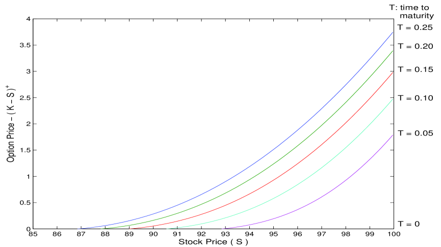
Figure 1. The option price function $S\rightarrow V(S,0)$ smoothly fits the pay-off function $(K-S)^{+}$ at $s(0)$. $V(S,0)$ increases and $s(0)$ ($V(S,0)-(K-S)^{+}=0$ at s(0)) decreases as time to maturity $T$ increases.

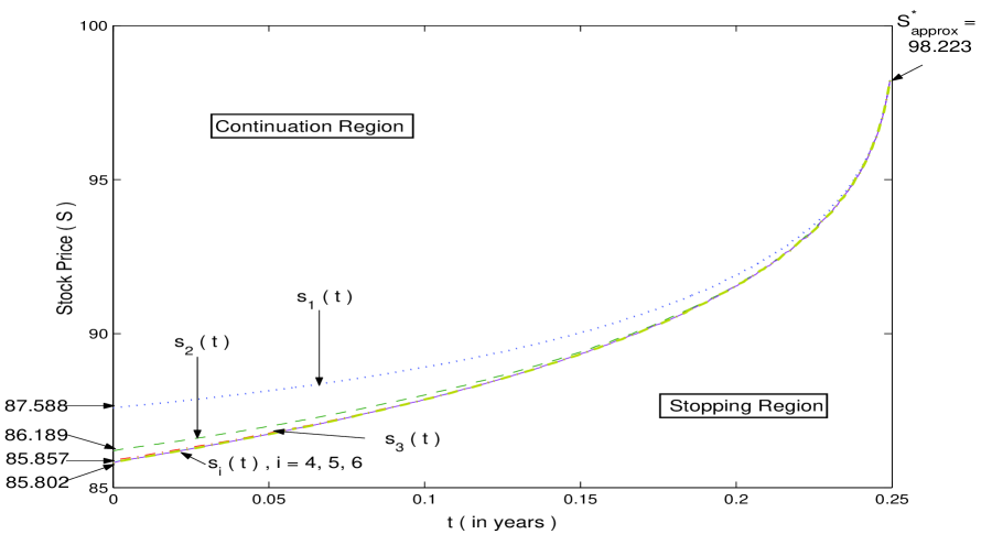
Figure 2. Iteration of the Exercise Boundary: $s_{n}(t)\downarrow s(t)$, $t\in[0,T)$. Both $s_{n}(t)$ and $s(t)$ will converge to $S^{*}<K$ as $t\rightarrow T$.

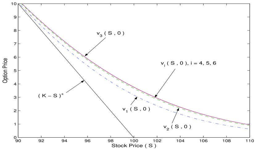
Figure 3. Iteration of the price functions: $v_{n}(S,0)\uparrow V(S,0)$, $S\geq 0$.

Next, we illustrate the behavior of the sequence of functions $\{v_{n}(S,t)\}_{n\geq 0}$ and its limit $V$ in Figures 1, 2 and 3. All the figures are obtained for an American put option in the case of the double exponential jump with $K=100$, $S_{0}=100$, $T=0.25$, $r=0.05$, $\sigma=0.2$, $\lambda=3$, $p=0.6$, $\eta_{1}=25$ and $\eta_{2}=25$ (the same parameters are used in the 8th row of Table 1) at a single run.

Remark 4.2.

1. In Figure 1, we show, how $V(S,0)$ depends on the time to maturity, and that it fits smoothly to the put-pay-off function at $s(0)$ (the exercise boundary). The $y$-axis is the difference between the option price and the pay-off function. As the time to maturity increases, the option price $V(S,0)$ increases while the exercise boundary $s(0)$ decreases. Even though the stock price process has jumps, the option price smoothly fits the pay-off function at $s(0)$, as in the classical Black-Scholes case without the jumps.

2. In Figure 2, we illustrate the convergence of the exercise boundaries $t\rightarrow s_{n}(t)$, $n\geq 1$. We can see from the figure that all $s_{n}(t)$ are convex functions. Also, the sequence $\{s_{n}\}_{n\geq 1}$ is a monotone decreasing sequence, which implies that the continuation region is getting larger, and that the convergence of the free boundary sequence is fast.

   Moreover, we notice that, when the parameters are chosen such that (2.12) is satisfied, the free boundaries are discontinuous at the maturity time. In addition, we have $s(T-)=s_{n}(T-)=S^{*}<K$, where $S^{*}$ is the unique solution of (2.14). Furthermore, if $F$ is the double exponential distribution as in (4.1), the integral equation (2.14) can be solved analytically to obtain

   $$S^{*}=\left(\frac{(\eta_{1}-1)r}{\lambda p}\right)^{1/\eta_{1}}\cdot K.$$ (4.5)

   With the parameters we choose, we get from (4.5) that $S^{*}=98.39$. It is close to our numerical result as one can see from Figure 2.

3. In Figure 3, we illustrate the convergence of the sequence of prices $\{v_{n}(S,0)\}_{n\geq 0}$. Observe that this is a monotonically increasing sequence and it converges to its limit $V(S,0)$ very fast.

Acknowledgment We are grateful to the two anonymous referees for their detailed comments that helped us improve our paper.

Table 1. Comparison between the proposed iterated jump algorithm with the method in [17] and [16], where the parameters were chosen as $r=0.05$, $S(0)=100$ and $p=0.6$. Amin’s price is calculated in [17] using the enhanced binomial tree method as in [3]. The accuracy of Amin’s price is up to about a penny. The KPW 5EXP price from [16] is calculated on a Pentium IV, 1.8 GHz, while the iterated price is calculated on Pentium IV, 3.0GHz, both using C++ implementation. Run times are in seconds. For numerical algorithm we propose, the number of grid points in $x$ is chosen as $2^{6}$ and $\Delta t=\Delta x$. The option prices from both Iterated Brennan-Schwartz and Iterated PSOR are the same. Below “B-S” stands for the Brennan-Schwartz.

American Put Double Exponential Jump Diffusion Model
Parameter Values						Amin’s	KW		KPW 5EXP			Proposed Algorithm
K	T	$\sigma$	$\lambda$	$\eta_{1}$	$\eta_{2}$	Price	Value	Error	Value	Error	Time	Value	Error	B-S Time	PSOR Time
90	0.25	0.2	3	25	25	0.75	0.76	0.01	0.74	-0.01	3.21	0.75	0	0.08	0.12
90	0.25	0.2	3	25	50	0.65	0.66	0	0.65	0	3.25	0.66	0.01	0.08	0.12
90	0.25	0.2	3	50	25	0.68	0.69	0.01	0.68	0	2.97	0.69	0.01	0.08	0.12
90	0.25	0.2	3	50	50	0.59	0.60	0.01	0.59	0	2.89	0.59	0	0.12	0.12
90	0.25	0.3	3	25	25	1.92	1.93	0.01	1.92	0	2.40	1.93	0.01	0.09	0.13
90	0.25	0.2	7	25	25	1.03	1.04	0.01	1.02	-0.01	3.18	1.03	0	0.12	0.17
90	0.25	0.3	7	25	25	2.19	2.20	0.01	2.18	-0.01	2.97	2.20	0.01	0.12	0.20
100	0.25	0.2	3	25	25	3.78	3.78	0	3.77	-0.01	3.08	3.78	0	0.12	0.12
100	0.25	0.2	3	25	50	3.66	3.66	0	3.65	-0.01	3.29	3.66	0	0.10	0.12
100	0.25	0.2	3	50	25	3.62	3.62	0	3.62	0	2.88	3.63	0.01	0.09	0.12
100	0.25	0.2	3	50	50	3.50	3.50	0	3.50	0	3.00	3.50	0	0.13	0.12
100	0.25	0.3	3	25	25	5.63	5.62	-0.01	5.63	0	2.44	5.63	0	0.13	0.15
100	0.25	0.2	7	25	25	4.26	4.27	0.01	4.26	0	3.48	4.27	0.01	0.17	0.17
100	0.25	0.3	7	25	25	5.99	5.99	0	5.99	0	2.95	6.00	0.01	0.17	0.18
90	1	0.2	3	25	25	2.91	2.96	0.05	2.90	-0.01	2.43	2.92	-0.01	0.63	0.78
90	1	0.2	3	25	50	2.70	2.75	0.05	2.69	-0.01	2.38	2.70	0	0.69	0.81
90	1	0.2	3	50	25	2.66	2.72	0.06	2.67	0.01	2.55	2.68	0.02	0.64	0.82
90	1	0.2	3	50	50	2.46	2.51	0.05	2.45	-0.01	2.30	2.45	-0.01	0.68	0.82
90	1	0.3	3	25	25	5.79	5.85	0.06	5.79	0	2.48	5.77	-0.02	0.70	0.94

Table 2. Option price in Merton jump-diffusion model

K=100, T=0.25, r=0.05, $\sigma=0.15$, $\lambda=0.1$. Stock price has lognormal jump distribution with $\tilde{\mu}=-0.9$ and $\tilde{\sigma}=0.45$. For the iterated jump schemes, the number of grid points in $x$ is chosen as $2^{7}$ and $\Delta t=\Delta x$. Below “B-S” stands for the Brennan-Schwartz.

Option Type	S(0)	dFLV	Proposed Algorithm
			Value	Error	LU(B-S) Time	PSOR Time
American Put	90	10.004	10.004	0	0.18	0.24
	100	3.241	3.242	0.001
	110	1.420	1.420	0
European Put	100	3.149	3.150	0.001	0.21	0.18
European Call	90	0.528	0.528	0	0.18	0.18
	100	4.391	4.392	0.001
	110	12.643	12.643	0

Table 3. European down-and-out barrier call option with Merton jump-diffusion model

K=110, S(0)=100, T=1, r=0.05, $\sigma=0.25$, $\lambda=2$, rebate R=1, the Stock price has lognormal jump distribution with $\tilde{\mu}=0$ and $\tilde{\sigma}=0.1$. For the algorithm we propose the number of grid points in $x$ is chosen as $2^{6}$ and $\Delta t=\Delta x$. Below we use the acronyms LU or SOR to tell wheher we use the LU factorization or the SOR to solve for the sparse linear systems at each time step.

Barrier H	MA Price	Proposed Algorithm
		Value	Error	LU Time	SOR Time
85	9.013	8.988	-0.025	0.52	0.71
95	5.303	5.290	-0.013	0.64	0.86

Table 4. Convergence of the numerical algorithm with respect to grid sizes

K=100, T=0.25, r=0.05, $\sigma=0.15$, $\lambda=0.1$, stock price has lognormal jump distribution with $\tilde{\mu}=-0.9$ and $\tilde{\sigma}=0.45$ (the same parameters that are used in [11]). The differential equation is discretized by the Crank-Nicolson scheme as (3.10) with $\theta=1/2$. The logarithmic variable $x=\log S$ is equally spaced discretized on an interval $[x_{min},x_{max}]$ with $\Delta x=\Delta t$. The numerical integral is truncated on the smallest interval $[z_{min},z_{max}]$, such that $[x+\tilde{\mu}-4\tilde{\sigma},x+\tilde{u}+4\tilde{\sigma}]$ will be inside $[z_{min},z_{max}]$ for any $x\in[x_{min},x_{max}]$. The step length for the numerical integral is chosen the same as the step length in $x$, i.e. $\Delta z=\Delta x$. The number of grid points for to implement the FFT is chosen as an integral power of 2. The error tolerance for PSOR method is $10^{-8}$ and for the global iteration is $10^{-6}$. Run times are in seconds. Each row in the “Difference” column of the following table is $v_{PSOR}(L,M)-v_{PSOR}(L/2,M/2)$. “B-S” stands for the Brennan-Schwartz algorithm. The number of global iteration is 3 for all the following numerical experiments.

S(0)	No. of grid	No. of time	B-S Value	B-S	PSOR Value	Difference	PSOR	Max. No. of
	points in $x$ ( L )	steps ( M )	$v_{B-S}$	Time	$v_{PSOR}$		Time	PSOR iterations
90	64	30	10.00230	0.06	10.00573	n.a.	0.06	16
	128	58	10.00142	0.21	10.00429	-0.00144	0.24	21
	256	115	10.00192	0.84	10.00396	-0.00033	0.99	28
	512	230	10.00218	3.51	10.00387	-0.00009	4.50	39
100	64	30	3.24074	0.06	3.24465	n.a.	0.06	16
	128	58	3.24008	0.21	3.24180	-0.00285	0.24	21
	256	115	3.24046	0.84	3.24115	-0.00065	0.99	28
	512	230	3.24058	3.51	3.24103	-0.00012	4.50	39
110	64	30	1.42048	0.06	1.42146	n.a.	0.06	16
	128	58	1.41941	0.21	1.41991	-0.00155	0.24	21
	256	115	1.41958	0.84	1.41966	-0.00025	0.99	28
	512	230	1.41962	3.51	1.41960	-0.00006	4.50	39

Using (4.4), the number of SOR iterations can be calculated. The calculation gives $11,16,22$ and $31$. Comparing with the last column of above table, the maximum numbers of PSOR iteration are slightly larger than these theoretical predicted SOR iteration times. Moreover, when $L=512$ the the ratio between the maximum number of PSOR iteration and $\sqrt{L}$ is 1.72. This confirms the analysis in Remark 4.1 that the maximal PSOR iteration time grows as the order of $\sqrt{L}$.

The parameters for the following three figures are $K=100$, $S_{0}=100$, $T=0.25$, $r=0.05$, $\sigma=0.2$, $\lambda=3$, the stock price has double exponential jump with $p=0.6$, $\eta_{1}=25$ and $\eta_{2}=25$ (the same parameters used in the 8th row of Table 1).

References

- [1] F. Aitsahlia and A. Runnemo. A canonical optimal stopping problem for American options under a double-exponential jump-diffusion model. Journal of Risk, 10:85–100, 2007.
- [2] A. Almendral and C. Oosterlee. On American options under the variance gamma process. Applied Mathematical Finance, 14(2):131–152, 2007.
- [3] K. I. Amin. Jump diffusion option valuation in discrete time. Journal of Finance, 48:1833 – 1863, 1993.
- [4] L. Andersen and J. Andreasen. Jump-diffusion processes: Volatility smile fitting and numerical methods for option pricing. Review of Derivatives Research, 4(3):231 – 262, 2000.
- [5] G. Barone-Adesi and R. E. Whaley. Efficient analytic approximation of American option values. Journal of Finance, 42:301 – 320, 1987.
- [6] E. Bayraktar. A proof of the smoothness of the finite time horizon American put option for jump diffusions. To appear in the SIAM Journal on Control and Optimization, 2008. Available at http://arxiv.org/abs/math.OC/0703782.
- [7] E. Bayraktar and H. Xing. Analysis of the optimal exercise boundary of American options for jump diffusions. Technical report, University of Michigan, 2008. Available at http://arxiv.org/abs/0712.3323.
- [8] M. J. Brennan and E. S. Schwartz. The valuation of American put options. Journal of Finance, 32(2):449 – 462, 1977.
- [9] R. Cont and E. Voltchkova. A finite difference scheme for option pricing in jump diffusion and exponential Lévy models. SIAM Journal on Numerical Analysis, 43(4):1596 – 1626, 2005.
- [10] Rama Cont and Peter Tankov. Financial modelling with jump processes. Chapman & Hall/CRC Financial Mathematics Series. Chapman & Hall/CRC, Boca Raton, FL, 2004.
- [11] Y. d’Halluin, P. A. Forsyth, and G. Labahn. A penalty method for American options with jump diffusion processes. Numerische Mathematik, 97(2):321–352, 2004.
- [12] Y. d’Halluin, P. A. Forsyth, and K. R. Vetzal. Robust numerical methods for contingent claims under jump diffusion processes. IMA Journal of Numerical Analysis, 25(1):87–112, 2005.
- [13] A. Hirsa and D. Madan. Pricing American options under variance gamma. Journal of Computational Finance, 7(2):63 – 80, 2004.
- [14] Kenneth R. Jackson, Sebastian Jaimungal, and Vladimir Surkov. Fourier space time stepping for option pricing with Lévy models. To appear in the Journal of Computational Finance, 2008.
- [15] P. Jaillet, D. Lamberton, and B. Lapeyre. Variational inequalities and the pricing of American options. Acta Applicandae Mathematicae, 21(3):263–289, 1990.
- [16] S. G. Kou, G. Petrella, and H. Wang. Pricing path-dependent options with jump risk via laplace transforms. Kyoto Economic Review, 74:1–23, 2005.
- [17] S. G. Kou and H. Wang. Option pricing under a double exponential jump diffusion model. Management Science, 50:1178–1192, 2004.
- [18] R. C. Merton. Option pricing when the underlying stock returns are discontinuous. Journal of Financial Economics, 3:125–144, 1976.
- [19] S. A. K. Metwally and A. F. Atiya. Fast monte carlo valuation of barrier options for jump diffusion processes. Proceesings of the Computational Intelligence for Financial Engineering, pages 101 – 107, 2003.
- [20] Paul Wilmott, Sam Howison, and Jeff Dewynne. The mathematics of financial derivatives. Cambridge University Press, Cambridge, 1995. A student introduction.
- [21] C. Yang, L. Jiang, and B. Bian. Free boundary and American options in a jump-diffusion model. European Journal of Applied Mathematics, 17(1):95–127, 2006.
- [22] D. M. Young. Iterative solution of large linear system. Academic Press, New York, 1971.
- [23] X. L. Zhang. Valuation of American options in a jump-diffusion model. In Numerical methods in finance, Publ. Newton Inst., pages 93–114. Cambridge Univ. Press, Cambridge, 1997.