Arrival time distribution for a driven system containing quenched dichotomous disorder

Abstract

We study the arrival time distribution of overdamped particles driven by a constant force in a piecewise linear random potential which generates the dichotomous random force. Our approach is based on the path integral representation of the probability density of the arrival time. We explicitly calculate the path integral for a special case of dichotomous disorder and use the corresponding characteristic function to derive prominent properties of the arrival time probability density. Specifically, we establish the scaling properties of the central moments, analyze the behavior of the probability density for short, long, and intermediate distances. In order to quantify the deviation of the arrival time distribution from a Gaussian shape, we evaluate the skewness and the kurtosis.

I Introduction

The overdamped equation of motion of a classical particle in one dimension presents a simple yet very useful model for the study of many physical, biological, economical, and other systems. Depending on the character of the force field acting on the particle, this equation provides a basis for describing different phenomena in these systems. Specifically, if the force field contains the noise terms arising from the influence of the environment, it describes a large variety of noise-induced phenomena including noise-induced transitions HL , directed transport Trans , and stochastic resonance GHJM , to name only a few. It should be noted that in some cases, especially within the white-noise approximation, the statistical properties of the solution of this equation can be obtained analytically.

If the environment is disordered the force field contains also the random functions of the spatial variable. In this case the overdamped dynamics represents both the noise-induced and disorder-induced effects and it can exhibit as well anomalous behavior even in the simplest situation of additive white noise BG . For the latter situation a number of exact results was obtained for Sinai disorder BG ; Sin ; Der ; Gol ; Mon , Gaussian disorder HTB ; Sch ; DV ; GB ; LV , and also for some special cases of non-Gaussian disorder Den ; DL ; PKDK ; KKDP ; DH .

When the noise terms produced by a stochastic environment become negligible, the overdamped equation of motion accounts solely for effects of quenched disorder. This equation effectively describes, e.g., the transport of particles in deterministic ratchets with quenched disorder PASF ; GLZH ; ZLAF and can be used for the study of the dynamics of localized structures like domain walls in random magnets and vortices in type-II superconductors. Although temporal noise terms are absent, there are only very few exact results available. Therefore, in order to fill this gap, we have examined the following dimensionless equation of motion for an overdamped particle DKDH :

$$\dot{X}_{t}=f+g(X_{t}).$$ (1)

Here, $X_{t}$ denotes the particle coordinate that satisfies the initial condition $X_{0}=0$, $f\,(>0)$ is a constant force, and $g(x)=-dU(x)/dx=\pm g$ is a dichotomous random force generated by a piecewise linear random potential $U(x)$, see Fig. 1. It is assumed that the random intervals $s_{j}$ of a linearly varying $U(x)$ are statistically independent and distributed with the same (exponential) probability density $p(s)$. Moreover, we assume that the conditions $f>g$ and $g(+0)=-g$ are imposed.

Equation (1) is of minimal form that accounts for the effects of quenched disorder on the overdamped motion of driven particles. Its main advantage is that many of the statistical properties of $X_{t}$ can be described analytically in full detail. Nevertheless, if the odd and even intervals $s_{j}$ are distributed with different exponential densities (in this case the exact results exist as well), then Eq. (1.1) can be used also for studying a number of important physical issues. Specifically, this equation constitutes a basis for describing the adiabatic transport of particles in randomly perturbed one-dimensional channels and presents a simple model for studying the low-temperature dynamics of charge carriers and localized structures in randomly layered media. In addition to the listed examples, we point out at rather unexpected application of Eq. (1.1) in astrophysics. Namely, if the clouds in interstellar space are distributed uniformly then the distances between them are distributed with an exponential distribution. In this case, assuming that the light velocity in the clouds is the same and the sizes of clouds are distributed with an exponential distribution, Eq. (1.1) can be used for studying the statistical properties of distances that pass the light emitted by a star in different directions.

In DKDH we derived the probability density of the solution of Eq. (1) and investigated explicitly its time evolution. In contrast, in this work we focus on the statistical properties of the arrival time for the particles governed by Eq. (1). The paper is structured as follows. In Sec. II, we derive the path integral representation for the probability density of the arrival time. The characteristic function of the arrival time is determined in Sec. III. In Sec. IV, we calculate the moments of the arrival time and study their asymptotic and scaling behavior. The basic properties of the arrival time probability density are studied in Sec. V, both analytically and numerically. We summarize our findings in Sec VI. Some technical details of our calculations are deferred to the Appendix.

II PATH INTEGRAL REPRESENTATION OF THE ARRIVAL TIME PROBABILITY DENSITY

According to Eq. (1), the arrival time $t_{x}$, i.e., the time that a particle spends moving from the origin to a position $x(>0)$, is given by the integral expression

$$t_{x}=\int_{0}^{x}\frac{dx}{f+g(x)}.$$ (2)

This time depends on the random function $g(x)$ and thus presents a random quantity. The probability density $P_{x}(t)$ that $t_{x}=t$ for a fixed coordinate $x$, i.e., the probability density of the arrival time, is defined in the well-known way as

$$P_{x}(t)=\langle\delta(t-t_{x})\rangle,$$ (3)

where the angular brackets denote an averaging over the sample paths of $g(x)$, and $\delta(t-t_{x})$ is the Dirac $\delta$ function.

To obtain the explicit form of $P_{x}(t)$ we use a path integral approach. Because of the dichotomous character of the random function $g(x)$, it is convenient to present the probability density in terms of the partial densities

$$P_{x}(t)=\sum_{n=0}^{\infty}P_{x}^{(n)}(t),$$ (4)

where $P_{x}^{(n)}(t)$ is the probability density that for the sample paths of $g(x)$ which are undergoing $n$ changes of the sign on the interval $(0,x)$ the condition $t_{x}=t$ holds. For a given $n\,(\geq 1)$ the solution of Eq. (1) can be written in the form

$$X_{t}^{(n)}=\sum_{j=1}^{n}s_{j}+\tilde{s}_{n+1}$$ (5)

with $\tilde{s}_{n+1}\in(0,s_{n+1})$. On the other hand, because $g(x)=(-1)^{j}g$ if $x$ belongs to the interval $s_{j}$, (2) yields

$$t_{x}^{(n)}=\sum_{j=1}^{n}\frac{s_{j}}{f+(-1)^{j}g}+\frac{\tilde{s}_{n+1}}{f+(-1)^{n+1}g}.$$ (6)

Setting $X_{t}^{(n)}=x$ and replacing $\tilde{s}_{n+1}$ by $x-\sum_{j=1}^{n}s_{j}$, the result (6) can be recast to

$$t_{x}^{(n)}=\frac{x}{f-(-1)^{n}g}-\frac{g}{f^{2}-g^{2}}\sum_{j=1}^{n}[(-1)^{n}+(-1)^{j}]s_{j}.$$ (7)

Let us next introduce the probability $p(s_{j})ds_{j}$ that the $j$-th jump of $g(x)$ occurs in the interval $ds_{j}$ and also the probability $\int_{l}^{\infty}p(s)ds$ that the distance between the nearest-neighbor jumps exceeds $l$. Then, the probability $dW_{n}(x)$ that the function $g(x)$ on the interval $(0,x)$ experiences $n$ jumps in the intervals $ds_{j}$ ($j=1,\ldots,n$) assumes the form

$$dW_{n}(x)=\int_{x-\sum_{j=1}^{n}s_{j}}^{\infty}p(s)ds\prod_{j=1}^{n}p(s_{j})ds_{j}.$$ (8)

Because $\tilde{s}_{n+1}>0$, the positive variables of integration, $s_{j}$, must satisfy the condition $\sum_{j=1}^{n}s_{j}<x$. Denoting by $\Omega_{n}(x)$ a region in the $n$-dimensional space of these variables, being defined by the aforementioned condition, we obtain

$$P_{x}^{(n)}(t)=\int_{\Omega_{n}(x)}\delta(t-t_{x}^{(n)})dW_{n}(x).$$ (9)

Finally, taking into account that $t_{x}^{(0)}=x/(f-g)$ is the arrival time at $n=0$ and $W_{0}(x)=\int_{x}^{\infty}p(s)ds$ is the total probability of those sample paths of $g(x)$ which do not change sign on the interval $(0,x)$, we end up with the following path integral representation for the probability density of the arrival time:

$$P_{x}(t)=\delta(t-t_{x}^{(0)})W_{0}(x)+\sum_{n=1}^{\infty}\int_{\Omega_{n}(x)}\delta(t-t_{x}^{(n)})dW_{n}(x).$$ (10)

This form of the arrival time probability density is rather general, but possesses a rather complex mathematical structure. Based on (10), however, we arrive at two conclusions that are valid for an arbitrary probability density $p(s)$: (i) $P_{x}(t)$ at a fixed $x$ is concentrated on the interval $[x/(f+g),x/(f-g)]$, and (ii) $P_{x}(t)$ is properly normalized, i.e., $\int_{0}^{\infty}P_{x}(t)dt=1$. Indeed, since $\min{t_{x}^{(n)}}=x/(f+g)$ and $\max{t_{x}^{(n)}}=x/(f-g)$, we have $\delta(t-t_{x}^{(n)})\equiv 0$ and so $P_{x}(t)\equiv 0$ if $t\notin[x/(f+g),x/(f-g)]$. To prove the second assertion, we first note that, according to (10), $\int_{0}^{\infty}P_{x}(t)dt=W_{0}(x)+\sum_{n=1}^{\infty}W_{n}(x)$, where $W_{n}(x)=\int_{\Omega_{n}(x)}dW_{n}(x)$ is the probability that the function $g(x)$ has undergone $n$ jumps in the interval $(0,x)$. Next, introducing the quantities $S_{n}(x)=\int_{\Omega_{n}(x)}\prod_{j=1}^{n}p(s_{j})ds_{j}$, we find the representations $W_{0}(x)=1-S_{1}(x)$ and $W_{n}(x)=S_{n}(x)-S_{n+1}(x)$, see also DKDH . Finally, taking into account that $S_{\infty}(x)=0$ and $\sum_{n=1}^{\infty}W_{n}(x)=S_{1}(x)$, we assure that the normalization condition holds true for an arbitrary $p(s)$.

III CHARACTERISTIC FUNCTION OF THE ARRIVAL TIME

By use of the integral formula for the $\delta$ function,

$$\delta(t-t_{x}^{(n)})=\frac{1}{2\pi}\int_{-\infty}^{\infty}e^{-i\omega(t-t_{x}^{(n)})}d\omega,$$ (11)

we can rewrite the probability density (10) in the form of a Fourier integral, i.e.,

$$P_{x}(t)=\frac{1}{2\pi}\int_{-\infty}^{\infty}\phi_{x}(\omega)\,e^{-i\omega t}d\omega.$$ (12)

According to Eqs. (10)–(12), the characteristic function $\phi_{x}(\omega)$, which determines all the statistical properties of the arrival time $t_{x}$, is obtained as

$$\phi_{x}(\omega)=e^{i\omega t_{x}^{(0)}}W_{0}(x)+\tilde{\phi}_{x}(\omega),$$ (13)

where

$$\tilde{\phi}_{x}(\omega)=\sum_{n=1}^{\infty}\int_{\Omega_{n}(x)}e^{i\omega t_{x}^{(n)}}dW_{n}(x).$$ (14)

In the general case of an arbitrary $p(s)$, the characteristic function has a complex structure involving an integration over the $n$-dimensional domain $\Omega_{n}(x)$ and a summation over all $n$. Remarkably, however, $\phi_{x}(\omega)$ can be expressed in terms of elementary functions if the random intervals $s_{j}$ are exponentially distributed, i.e., if $p(s)=\lambda e^{-\lambda s}$, where $\lambda^{-1}$ is the average length of $s_{j}$. In this case the probability (8) becomes

$$dW_{n}(x)=e^{-\lambda x}\lambda^{n}\prod_{j=1}^{n}ds_{j},$$ (15)

and (14) reduces to

$$\tilde{\phi}_{x}(\omega)=e^{-\lambda x}\sum_{n=1}^{\infty}\lambda^{n}\int_{\Omega_{n}(x)}e^{i\omega t_{x}^{(n)}}\prod_{j=1}^{n}ds_{j}.$$ (16)

For the calculation of $\tilde{\phi}_{x}(\omega)$ it is convenient to transform the right-hand side of Eq. (16) into a form with separate integrations over the variables $s_{j}$. To this end, we use an approach DKDH based on the integral representation of the step function

$$\frac{1}{2\pi}\int_{-\infty}^{+\infty}\frac{e^{(i\kappa+\eta)y}}{i\kappa+\eta}\,d\kappa=\left\{\begin{array}[]{ll}1\;\;\textrm{if}\;y>0\\[6.0pt] 0\;\;\textrm{if}\;y<0\end{array}\right.$$ (17)

which is valid for arbitrary $\eta>0$. Applying (17) to (16) and setting $y=x-\sum_{j=1}^{n}s_{j}$, one obtains the desired result:

$$\tilde{\phi}_{x}(\omega)\!\! = \!\!\frac{e^{-\lambda x}}{2\pi}\sum_{n=1}^{\infty}\lambda^{n}\int_{-\infty}^{\infty}d\kappa\frac{e^{(i\kappa+\eta)x}}{i\kappa+\eta}\int_{0}^{\infty}\!\!\ldots\!\int_{0}^{\infty}\!e^{i\omega t_{x}^{(n)}}$$ (18)

$$\!\!\times e^{-(i\kappa+\eta)\sum_{j=1}^{n}s_{j}}\prod_{j=1}^{n}ds_{j}.$$

Then, using the identity $\sum_{n=1}^{\infty}a_{n}=\sum_{m=1}^{\infty}[a_{2m-1}+a_{2m}]$ and taking into account that, according to (7),

$$\displaystyle t_{x}^{(2m-1)}=\frac{x}{f+g}+\frac{2g}{f^{2}-g^{2}}\sum_{j=1}^{m}s_{2j-1},$$

$$\displaystyle t_{x}^{(2m)}=\frac{x}{f-g}-\frac{2g}{f^{2}-g^{2}}\sum_{j=1}^{m}s_{2j},$$ (19)

we reduce the formula (18) to the form

$$\tilde{\phi}_{x}(\omega)\!\! = \!\!\frac{e^{-\lambda x}}{2\pi}\int_{-\infty}^{\infty}\!\frac{e^{\nu_{0}x}}{\nu_{0}}\sum_{m=1}^{\infty}\Big{[}I^{m-1}(\nu_{0})I^{m}(\nu_{1})e^{i\omega x/(f+g)}$$ (20)

$$\!\!+\,I^{m}(\nu_{0})I^{m}(\nu_{2})e^{i\omega x/(f-g)}\Big{]}d\kappa.$$

Here,

$$I(\nu_{k})=\int_{0}^{\infty}p(s)e^{-(\nu_{k}-\lambda)s}ds=\frac{\lambda}{\nu_{k}}$$ (21)

($\text{Re}\,\nu_{k}>0$, $k=0,1,2$) and

$$\nu_{k}=i\kappa+\eta+i\frac{2q\omega}{f^{2}-g^{2}}\delta_{k}$$ (22)

with $\delta_{0}=0$, $\delta_{1}=-1$, and $\delta_{2}=1$. We note that the right-hand side of (20) contains an arbitrary positive parameter $\eta$. According to the definition (14), however, the left-hand side of (20) does not depend on $\eta$. This implies that the final result of evaluating the series and integral in (20) does not depend on $\eta$ as well. Therefore, for auxiliary manipulations we may choose a most convenient value for this parameter.

From this point of view, it is reasonable to choose $\eta>\lambda$. This is so because in this case $|I(\nu_{k})|<1$ and the series in (20) can be easily evaluated:

$$\displaystyle\sum_{m=1}^{\infty}I^{m-1}(\nu_{0})I^{m}(\nu_{1})=\frac{\lambda\nu_{0}}{\nu_{0}\nu_{1}-\lambda^{2}},$$

$$\displaystyle\sum_{m=1}^{\infty}I^{m}(\nu_{0})I^{m}(\nu_{2})=\frac{\lambda^{2}}{\nu_{0}\nu_{2}-\lambda^{2}}.$$ (23)

Substituting (23) into (20) and using that $W_{0}(x)=e^{-\lambda x}$ and

$$e^{i\omega t_{x}^{(0)}}W_{0}(x)=\frac{e^{-\lambda x}}{2\pi}\int_{-\infty}^{\infty}\frac{e^{\nu_{0}x}}{\nu_{0}}\,e^{i\omega x/(f-g)}d\kappa,$$ (24)

from (13) we obtain

$$\phi_{x}(\omega)=\frac{e^{-\lambda x}}{2\pi}\int_{-\infty}^{\infty}e^{\nu_{0}x}\bigg{[}\frac{\lambda e^{i\omega x/(f+g)}}{\nu_{0}\nu_{1}-\lambda^{2}}+\frac{\nu_{2}e^{i\omega x/(f-g)}}{\nu_{0}\nu_{2}-\lambda^{2}}\bigg{]}d\kappa.$$ (25)

Upon calculating the integrals in (25) (the details are given in the Appendix) we find a remarkably simple expression for the characteristic function of the arrival time

$$\phi_{x}(\omega)\!\! = \!\!e^{-\lambda x(1-i\nu f/g)}\bigg{[}\cosh\Big{(}\lambda x\sqrt{1-\nu^{2}}\Big{)}$$ (26)

$$\!\!+\,\frac{1+i\nu}{\sqrt{1-\nu^{2}}}\sinh\Big{(}\lambda x\sqrt{1-\nu^{2}}\Big{)}\bigg{]},$$

where

$$\nu=\frac{\omega g}{\lambda(f^{2}-g^{2})}.$$ (27)

We note that $\phi_{x}(\omega)$, being the characteristic function, satisfies the conditions $|\phi_{x}(\omega)|\leq 1$, $\phi_{x}(0)=1$ and $\phi_{x}(-\omega)=\phi_{x}^{*}(\omega)$, where the asterisk indicates the complex conjugation. Equation (26) is our main result which allows us to study the essential properties of the arrival time analytically.

IV MOMENTS OF THE ARRIVAL TIME

The moments of the arrival time are defined in the usual way as $\langle t_{x}^{m}\rangle=\int_{-\infty}^{\infty}t^{m}P_{x}(t)dt$, and can be deduced through the characteristic function as follows:

$$\langle t_{x}^{m}\rangle=\frac{1}{i^{m}}\frac{d^{m}}{d\omega^{m}}\,\phi_{x}(\omega)\Big{|}_{\omega=0}.$$ (28)

According to (26) and (28), the first moment, i.e., the mean arrival time, emerges as

$$\langle t_{x}\rangle=\frac{1}{2\lambda(f^{2}-g^{2})}\Big{[}2\lambda fx+g-ge^{-2\lambda x}\Big{]}.$$ (29)

At small distances from the origin, when $\lambda x\ll 1$, the formula (29) yields $\langle t_{x}\rangle=x/(f-g)$. This result is expected: The total probability of those sample paths of $g(x)$ which do not change the sign on the interval $(0,x)$ tends to 1 as $\lambda x\to 0$, and thus the average particle velocity tends to $f-g$. In the other limiting case, when $\lambda x\gg 1$, the formula (29) approaches $\langle t_{x}\rangle=fx/(f^{2}-g^{2})$. This result is corroborated by the fact that the long-time asymptotic of the average particle velocity equals $(f^{2}-g^{2})/f$ DKDH .

The moments of higher order can also be calculated straightforwardly. In particular, for the second moment we obtain

$$\langle t_{x}^{2}\rangle\!\! = \!\!\frac{1}{2\lambda^{2}(f^{2}-g^{2})^{2}}\Big{[}2\lambda^{2}f^{2}x^{2}+2\lambda g(f+g)x-g^{2}$$ (30)

$$\!\!-\,g(2\lambda fx-g)e^{-2\lambda x}\Big{]}.$$

The central moments, $\langle(t_{x}-\langle t_{x}\rangle)^{m}\rangle$, can be determined from the finite series

$$\langle(t_{x}-\langle t_{x}\rangle)^{m}\rangle=\sum_{j=0}^{m}(-1)^{m-j}C_{m}^{j}\langle t_{x}^{l}\rangle\langle t_{x}\rangle^{m-l},$$ (31)

where $C_{m}^{j}$ is the binomial coefficient, or, alternatively, by the formula

$$\langle(t_{x}-\langle t_{x}\rangle)^{m}\rangle=\frac{1}{i^{m}}\frac{d^{m}}{d\omega^{m}}\,\phi_{x}(\omega)\,e^{-i\omega\langle t_{x}\rangle}\Big{|}_{\omega=0}.$$ (32)

Specifically, using either of these definitions, the variance of the arrival time, $\sigma_{x}^{2}=\langle(t_{x}-\langle t_{x}\rangle)^{2}\rangle$, can be written in the form

$$\sigma_{x}^{2}=\frac{g^{2}}{4\lambda^{2}(f^{2}-g^{2})^{2}}\Big{[}4\lambda x-3+4e^{-2\lambda x}-e^{-4\lambda x}\Big{]}.$$ (33)

At short distances, when $\lambda x\ll 1$, the variance reduces to

$$\sigma_{x}^{2}=\frac{4\lambda g^{2}}{3(f^{2}-g^{2})^{2}}x^{3},$$ (34)

and at long distances, when $\lambda x\gg 1$, it reduces to

$$\sigma_{x}^{2}=\frac{g^{2}}{\lambda(f^{2}-g^{2})^{2}}x.$$ (35)

Moreover, the central moments of the arrival time possess interesting scaling properties. Namely, using (32) with (26) and (29), one obtains

$$\langle(t_{x}-\langle t_{x}\rangle)^{m}\rangle=\bigg{(}\frac{g}{\lambda(f^{2}-g^{2})}\bigg{)}^{m}\Psi_{m}(\lambda x),$$ (36)

where

$$\Psi_{m}(\lambda x)=e^{-\lambda x}\frac{d^{m}}{dz^{m}}\,\Phi(z,\lambda x)\Big{|}_{z=0}$$ (37)

is a function of the single variable $\lambda x$, and

$$\Phi(z,\lambda x)\!\! = \!\!\exp\bigg{(}-z\,\frac{1-e^{-2\lambda x}}{2}\bigg{)}\bigg{[}\cosh\Big{(}\lambda x\sqrt{1+z^{2}}\Big{)}$$ (38)

$$\!\!+\,\frac{1+z}{\sqrt{1+z^{2}}}\sinh\Big{(}\lambda x\sqrt{1+z^{2}}\Big{)}\bigg{]}.$$

Thus, the central moments exhibit a universal dependence on $f$, $g$ and $\lambda$, i.e., $\langle(t_{x}-\langle t_{x}\rangle)^{m}\rangle\propto[g/\lambda(f^{2}-g^{2})]^{m}$.

V PROPERTIES OF THE ARRIVAL TIME PROBABILITY DENSITY

As it follows from (26), the characteristic function tends to $e^{-\lambda x+i\omega x/(f-g)}$ as $|\omega|\to\infty$. According to (12), this suggests that the probability density of the arrival time contains the $\delta$-singular contribution, i.e.,

$$P_{x}(t)=\delta\left(t-\frac{x}{f-g}\right)e^{-\lambda x}+\tilde{P}_{x}(t),$$ (39)

where

$$\tilde{P}_{x}(t)=\frac{1}{2\pi}\int_{-\infty}^{\infty}\tilde{\phi}_{x}(\omega)e^{-i\omega t}d\omega$$ (40)

denotes the regular part of $P_{x}(t)$ and

$$\tilde{\phi}_{x}(\omega)=\phi_{x}(\omega)-e^{-\lambda x+i\omega x/(f-g)}.$$ (41)

Because the intensity of the $\delta$-singular part decreases exponentially with increasing $x$, its contribution to $P_{x}(t)$ plays a crucial role only at short distances from the origin. The regular part rules the behavior of $P_{x}(t)$ at longer distances.

V.1 Behavior at short distances

At $\lambda x\ll 1$ we can obtain the probability density $P_{x}(t)$ in a simple way, without the need to evaluate the integral in (40). To this end, we first note that the $\delta$-singular part of $P_{x}(t)$ is formed by those sample paths of $g(x)$ that do not change the sign on the interval $(0,x)$. Accordingly, only the sample paths which have at least one change of the sign on this interval do contribute to the regular part $\tilde{P}_{x}(t)$. For small values of $\lambda x$ repeated changes of the sign are unlikely. Therefore, in order to determine $\tilde{P}_{x}(t)$, we consider the sample paths with a single change of the sign. In this case the probability $\tilde{P}_{x}(t)dt$ is equal to $dW_{1}(x)=\lambda e^{-\lambda x}ds_{1}$ and, because $t=t_{x}^{(1)}=x/(f+g)+2gs_{1}/(f^{2}-g^{2})$, the relation $\tilde{P}_{x}(t)dt=dW_{1}(x)$ at $\lambda x\ll 1$ then yields

$$\tilde{P}_{x}(t)=\frac{\lambda(f^{2}-g^{2})}{2g}.$$ (42)

Finally, substituting (42) into (39), we find the probability density of the arrival time at $\lambda x\ll 1$:

$$P_{x}(t)=\delta\left(t-\frac{x}{f-g}\right)(1-\lambda x)+\frac{\lambda(f^{2}-g^{2})}{2g}.$$ (43)

At first sight, this result may come as a surprise because the regular part of the probability density does not depend explicitly on $x$ and $t$. It should be stressed, however, that the formula (42) is derived under the condition that $t\in[t_{\text{min}},t_{\text{max}}]$, where $t_{\text{min}}=x/(f+g)$ and $t_{\text{max}}=x/(f-g)$ [we recall that $\tilde{P}_{x}(t)\equiv 0$ if $t\notin[t_{\text{min}},t_{\text{max}}]$]. This means that $\tilde{P}_{x}(t)$ depends on $x$ and $t$ implicitly leading to the broadening of $\tilde{P}_{x}(t)$ if $x$ increases. At the starting point $x=0$ we have $t_{\text{min}}=t_{\text{max}}=0$, therefore $\tilde{P}_{0}(t)=0$ and, in accordance with the condition $t_{0}=0$, $P_{0}(t)=\delta(t)$. We note also that the normalization condition $\int_{t_{\text{ min}}}^{t_{\text{max}}}P_{x}(t)dt=1$, which holds true also for (43), further corroborates the validity of (42).

V.2 Behavior at long distances

To study the long-distance behavior of the probability density $P_{x}(t)$, it is convenient to introduce the new time variable $\tau=(t-\langle t_{x}\rangle)/\sigma_{x}$. The corresponding scaled probability density $\mathcal{P}_{x}(\tau)$ is expressed through $P_{x}(t)$ as $\mathcal{P}_{x}(\tau)=\sigma_{x}P_{x}(\langle t_{x}\rangle+\sigma_{x}\tau)$ and, according to (12), it can be written in the form

$$\mathcal{P}_{x}(\tau)=\frac{1}{2\pi}\int_{-\infty}^{\infty}\phi_{x}(\mu/\sigma_{x})\,e^{-i\mu\langle t_{x}\rangle/\sigma_{x}-i\mu\tau}d\mu.$$ (44)

Using (26), (29) and (33), the characteristic function of $\mathcal{P}_{x}(\tau)$ then reads

$$\phi_{x}(\mu/\sigma_{x})\,e^{-i\mu\langle t_{x}\rangle/\sigma_{x}}=e^{-\lambda x}\Phi(i\mu\Psi_{2}^{-1/2}(\lambda x),\lambda x),$$ (45)

where the function $\Phi(z,\lambda x)$ is defined by Eq. (38) and

$$\Psi_{2}(\lambda x)=\lambda x-\frac{3}{4}+e^{-2\lambda x}-\frac{1}{4}\,e^{-4\lambda x}.$$ (46)

Because the characteristic function (45) depends only on $\lambda x$ and the integration variable $\mu$, the scaled probability density (44) possesses the remarkable property that $\mathcal{P}_{x}(\tau)$ is a function of $\lambda x$ and $\tau$ which depends neither on the external force $f$ nor on the amplitude $g$ of the dichotomous random force $g(x)$.

In the case of long distances, if $\lambda x\gg 1$, the characteristic function (45) at $\mu^{4}\ll\lambda x$ can be approximated by the two terms of its expansion:

$$\phi_{x}(\mu/\sigma_{x})\,e^{-i\mu\langle t_{x}\rangle/\sigma_{x}}=e^{-\mu^{2}/2}\left(1-\frac{\mu^{4}}{8\lambda x}\right).$$ (47)

Substituting (47) into (45) and calculating the integrals, we find the two terms of expression of the scaled probability density

$$\mathcal{P}_{x}(\tau)=\frac{e^{-\tau^{2}/2}}{\sqrt{2\pi}}\left(1-\frac{3-6\tau^{2}+\tau^{4}}{8\lambda x}\right)$$ (48)

which is valid if $\lambda x\gg\max{(1,\tau^{4})}$. Thus, in accordance with the central limit theorem of probability theory (see, e.g., Ref. GK ), the limiting probability density approaches a Gaussian form, i.e., $\mathcal{P}_{\infty}(\tau)=(2\pi)^{-1/2}e^{-\tau^{2}/2}$, and $\mathcal{P}_{x}(\tau)-\mathcal{P}_{\infty}(\tau)\propto(\lambda x)^{-1}$ as $\lambda x\to\infty$.

V.3 Numerical verification

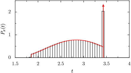
Figure 2: (Color online) Theoretical and simulated probability density of the arrival time for $x=2.4$. The solid line (red online) and histogram represent the analytical result (39) and the numerical simulation of the arrival time (2), respectively. The parameters of the force field are chosen as $f=1$, $g=0.3$, and $\lambda=1$. The vertical arrow depicts the $\delta$-singular contribution to $P_{x}(t)$.

Our numerical calculations pursue two goals, namely (i) to verify the analytical findings and (ii) to illustrate and visualize the obtained findings. The former is achieved by comparison of the probability density (39) with that derived from the numerical simulation of the arrival time (2). We use the Maple package for calculating the Fourier integral in (40) and employ the histogram procedure to numerically evaluate the probability density. In short, this procedure consists of successive generations of random intervals $s_{j}$ according to the exponential distribution and evaluating the arrival time to a fixed position $x$ for different realizations of random intervals. The probability density is then presented as the histogram of arrival times of the particle. For further details about this procedure we refer the interested reader to Ref. DKDH where a similar approach was used for the numerical evaluation of the probability density of the particle position at a fixed time $t$. In doing so, we made sure that the simulated probability density function is in perfect agreement with the theoretical one, see Fig. 2.

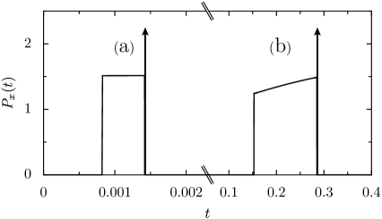
Figure 3: Short-distance behavior of the probability density of the arrival time $P_{x}(t)$ at (a) $x=10^{-3}$ and (b) $x=0.2$. The other parameters are the same as those in Fig. 2.

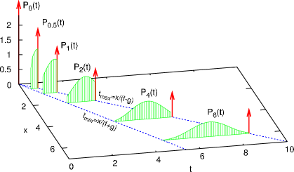
Figure 4: (Color online) Plots of the probability density of the arrival time for different distances from the origin of the coordinate system. The vertical surfaces (green online) depict the regular part of $P_{x}(t)$. In order to visually demonstrate that the intensity of the $\delta$-singular part of $P_{x}(t)$ exponentially decreases with $x$, we depicted the length of the vertical arrows (red online) in the form $0.8+2e^{-\lambda x}$. For the convenience of comparison, the force field characteristics are chosen as in Figs. 2 and 3.

Figure 3 illustrates the short-distance behavior of the probability density (39). As can be seen in Fig. 3(a), at very small values of $x$ the probability density of the arrival time is described by the approximate formula (43). In accordance with the assumption made in its derivation, this suggests that the sample paths of $g(x)$ which on the interval $(0,x)$ have more than one change of the sign are responsible for the explicit dependence of $\tilde{P}_{x}(t)$ on $t$. If $x$ is not too small, i.e., the total probability of these sample paths is small but non-zero, then, as shown in Fig. 3(b), $\tilde{P}_{x}(t)$ is an almost linear function of $t$. With increasing of $x$ the role of these sample paths becomes increasingly important: The function $\tilde{P}_{x}(t)$ becomes nonlinear, assumes a unimodal form, and eventually approaches a Gaussian shape, see Fig. 4.

V.4 Skewness and kurtosis

In order to quantitatively describe the difference between the arrival time probability density and a Gaussian density with identical mean and variance as $P_{x}(t)$, we calculate the skewness

$$s(x)=\frac{\langle(t_{x}-\langle t_{x}\rangle)^{3}\rangle}{\sigma_{x}^{3}}$$ (49)

that characterizes the degree of asymmetry of $P_{x}(t)$, and as well the kurtosis

$$k(x)=\frac{\langle(t_{x}-\langle t_{x}\rangle)^{4}\rangle}{\sigma_{x}^{4}}-3$$ (50)

that characterizes the degree of peakedness of $P_{x}(t)$. Because $s(x)\equiv 0$ and $k(x)\equiv 0$ if the arrival time $t_{x}$ follows a Gaussian distribution, one can consider the skewness and kurtosis as appropriate measures of deviation of the arrival time distribution from a Gaussian shape. Using the representation (36) for the central moments, from the definitions (49) and (50) we obtain

$$s(x)=\frac{\Psi_{3}(\lambda x)}{\Psi_{2}^{3/2}(\lambda x)},\quad k(x)=\frac{\Psi_{4}(\lambda x)}{\Psi_{2}^{2}(\lambda x)}-3,$$ (51)

i.e., $s(x)$ and $k(x)$ are universal functions of the single variable $\lambda x$, see Fig. 5. Calculating $\Psi_{3}(\lambda x)$ and $\Psi_{4}(\lambda x)$ and taking into account (46), we find an explicit expression for the skewness,

$$s(x)\!\! = \!\!-\frac{2}{(4\lambda x-3+4e^{-2\lambda x}-e^{-4\lambda x})^{3/2}}\,[2+(3$$ (52)

$$\!\!-\,12\lambda x)e^{-2\lambda x}-6e^{-4\lambda x}+e^{-6\lambda x}],$$

and for the kurtosis,

$$k(x)\!\! = \!\!\frac{6}{(4\lambda x-3+4e^{-2\lambda x}-e^{-4\lambda x})^{2}}\,[13-8\lambda x$$ (53)

$$\!\!-\,8(1+4\lambda x)e^{-2\lambda x}-4(3-4\lambda x)e^{-4\lambda x}$$

$$\!\!+\,8e^{-6\lambda x}-e^{-8\lambda x}].$$

The formulas (52) and (53) yield in leading order of $\lambda x$ the following relations: $s(x)=-(3\sqrt{3}/4)(\lambda x)^{-1/2}$ and $k(x)=(9/5)(\lambda x)^{-1}$ at $\lambda x\ll 1$, and $s(x)=-(1/2)(\lambda x)^{-3/2}$ and $k(x)=-3(\lambda x)^{-1}$ at $\lambda x\gg 1$. These results clearly evidence that the arrival time probability density $P_{x}(t)$ distinctly differs from a Gaussian density at short distances and approaches this Gaussian shape at long distances. Moreover, since $|k(x)/s(x)|\to\infty$ as both, $\lambda x\to 0$ and $\lambda x\to\infty$, the kurtosis can be considered as a unique measure of non-Gaussianity of $P_{x}(t)$. We note that, because of the condition $s(x)<0$, the left tail of $P_{x}(t)$ is always heavier than the right tail. Also, $P_{x}(t)$ is more peaked compared to the Gaussian density at distances where $k(x)>0$, and is more flattened at distances where $k(x)<0$.

VI CONCLUSIONS

We applied the path integral approach to calculate the characteristic function of the arrival time for overdamped particles driven by a constant bias in a piecewise linear random potential producing a dichotomous random force with exponentially distributed spatial intervals. Using the characteristic function, we derived the moments of the arrival time, established universal scaling properties of the central moments, and demonstrated that the arrival time probability density $P_{x}(t)$ contains both a $\delta$-singular contribution and a regular part. While the $\delta$-singular part, whose weight decreases exponentially with increasing $x$, plays the main role at short distances, the regular part of $P_{x}(t)$ dominates at large distances $x$.

At very small distances the regular part is defined by the sample paths with only one change of the sign on the interval $(0,x)$ and in this case its value does not depend on $x$. Upon increasing $x$ the contribution of other sample paths leads to the transformation of this part of $P_{x}(t)$ into an almost linear function of $t$, and subsequently into unimodal form, and finally, at $x\to\infty$, it tends to a Gaussian density as $x^{-1}$. Moreover, in order to characterize the difference of the arrival time probability density from the Gaussian density, we calculated the skewness and kurtosis. The function $P_{x}(t)$ is more peaked in comparison with the Gaussian density at small $x$ and is more flattened at large $x$.

Appendix A DERIVATION OF THE CHARACTERISTIC FUNCTION

For calculating the integrals in (25),

$$\displaystyle Y=\frac{1}{2\pi}\int_{-\infty}^{\infty}\frac{\lambda e^{\nu_{0}x}}{\nu_{0}\nu_{1}-\lambda^{2}}d\kappa,$$

$$\displaystyle Z=\frac{1}{2\pi}\int_{-\infty}^{\infty}\frac{\nu_{2}e^{\nu_{0}x}}{\nu_{0}\nu_{2}-\lambda^{2}}d\kappa,$$ (54)

we use the method of contour integration MF . According to (22) and (27), the integrands in (54), $R(\kappa)=\lambda e^{\nu_{0}x}/(\nu_{0}\nu_{1}-\lambda^{2})$ and $S(\kappa)=\nu_{2}e^{\nu_{0}x}/(\nu_{0}\nu_{2}-\lambda^{2})$, can be written in the form

$$\displaystyle R(\kappa)=-\frac{\lambda}{(\kappa-\kappa_{1})(\kappa-\kappa_{2})}\,e^{(i\kappa+\eta)x},$$

$$\displaystyle S(\kappa)=-\frac{i\kappa+\eta+2i\lambda\nu}{(\kappa-\kappa_{3})(\kappa-\kappa_{4})}\,e^{(i\kappa+\eta)x},$$ (55)

where

$$\kappa_{1,2}=i\eta\pm i\lambda\sqrt{1-\nu^{2}}+\lambda\nu,$$

$$\kappa_{3,4}=i\eta\pm i\lambda\sqrt{1-\nu^{2}}-\lambda\nu.$$ (56)

The formulas (55) exhibit that both $R(\kappa)$ and $S(\kappa)$ as functions of the complex variable $\kappa$ have two poles of the first order at $\kappa=\kappa_{1,2}$ and $\kappa=\kappa_{3,4}$, respectively. If $\eta>\lambda$ then all poles are located in the upper half plane of the complex $\kappa$ plane, and the residue theorem yields

$$Y=i[\text{Res}\,R(\kappa_{1})+\text{Res}\,R(\kappa_{2})],$$

$$Z=i[\text{Res}\,S(\kappa_{3})+\text{Res}\,S(\kappa_{4})].$$ (57)

Since the residues in (57) are defined as $\text{Res}\,R(\kappa_{1,2})=\lim_{\kappa\to\kappa_{1,2}}(\kappa-\kappa_{1,2})R(\kappa)$ and $\text{Res}\,S(\kappa_{3,4})=\lim_{\kappa\to\kappa_{3,4}}(\kappa-\kappa_{3,4})S(\kappa)$, from (55) and (56) we obtain

$$Y\!\! = \!\!\frac{1}{\sqrt{1-\nu^{2}}}\sinh\Big{(}\lambda x\sqrt{1-\nu^{2}}\Big{)}e^{i\lambda x\nu},$$

$$Z\!\! = \!\!\bigg{[}\frac{i\nu}{\sqrt{1-\nu^{2}}}\sinh\Big{(}\lambda x\sqrt{1-\nu^{2}}\Big{)}$$ (58)

$$\!\!+\,\cosh\Big{(}\lambda x\sqrt{1-\nu^{2}}\Big{)}\bigg{]}e^{-i\lambda x\nu}.$$

Finally, substituting (58) into the formula

$$\phi_{x}(\omega)=e^{-\lambda x}\Big{[}Ye^{i\omega x/(f+g)}+Ze^{i\omega x/(f-g)}\Big{]}$$ (59)

which follows from (25) and (54), we get the desired characteristic function (26).

Figure 1: Schematic representation of (a) the piecewise linear random potential $U(x)$ and (b) the corresponding dichotomous random force $g(x)=-dU(x)/dx$ as functions of the coordinate $x$.

Figure 5: Plots of the skewness $s(x)$ (dashed line) and the kurtosis $k(x)$ (solid line) of the arrival time probability density vs the normalized distance $\lambda x$.

References

• (1) W. Horsthemke and R. Lefever, Noise-Induced Transitions (Springer-Verlag, Berlin, 1984).
• (2) P. Reimann and P. Hänggi, Appl. Phys. A: Mater. Sci. Process. 75, 169 (2002); R. D. Astumian and P. Hänggi, Phys. Today 55 (11), 33 (2002); P. Hänggi, F. Marchesoni, and F. Nori, Ann. Phys. (Leipzig) 14, 51 (2005).
• (3) L. Gammaitoni, P. Hänggi, P. Jung, and F. Marchesoni, Rev. Mod. Phys. 70, 223 (1998).
• (4) J.-P. Bouchaud and A. Georges, Phys. Rep. 195, 127 (1990).
• (5) Ya. G. Sinai, Theor. Probab. Appl. 27, 256 (1982).
• (6) B. Derrida, J. Stat. Phys. 31, 433 (1983).
• (7) A. O. Golosov, Commun. Math. Phys. 92, 491 (1984).
• (8) C. Monthus, Lett. Math. Phys. 78, 207 (2006).
• (9) P. Hänggi, P. Talkner, and M. Borkovec, Rev. Mod. Phys. 62, 251 (1990), see Sec. VII, C.3.
• (10) S. Scheidl, Z. Phys. B 97, 345 (1995).
• (11) P. Le Doussal and V. M. Vinokur, Physica C 254, 63 (1995).
• (12) D. A. Gorokhov and G. Blatter, Phys. Rev. B 58, 213 (1998).
• (13) A. V. Lopatin and V. M. Vinokur, Phys. Rev. Lett. 86, 1817 (2001).
• (14) S. I. Denisov, J. Magn. Magn. Mater. 147, 406 (1995).
• (15) S. I. Denisov and R. Yu. Lopatkin, Phys. Scr. 56, 423 (1997).
• (16) P. E. Parris, M. Kuś, D. H. Dunlap, and V. M. Kenkre, Phys. Rev. E 56, 5295 (1997).
• (17) V. M. Kenkre, M. Kuś, D. H. Dunlap, and P. E. Parris, Phys. Rev. E 58, 99 (1998).
• (18) S. I. Denisov and W. Horsthemke, Phys. Rev. E 62, 3311 (2000).
• (19) M. N. Popescu, C. M. Arizmendi, A. L. Salas-Brito, and F. Family, Phys. Rev. Lett. 85, 3321 (2000).
• (20) L. Gao, X. Luo, S. Zhu, and B. Hu, Phys. Rev. E 67, 062104 (2003).
• (21) D. G. Zarlenga, H. A. Larrondo, C. M. Arizmendi, and F. Family, Phys. Rev. E 75, 051101 (2007).
• (22) S. I. Denisov, M. Kostur, E. S. Denisova, and P. Hänggi, Phys. Rev. E 75, 061123 (2007).
• (23) B. V. Gnedenko and A. N. Kolmogorov, Limit Distributions for Sums of Independent Random Variables (Addison-Wesley, Cambridge, MA, 1954).
• (24) P. M. Morse and H. Feshbach, Methods of Theoretical Physics (McGraw-Hill, New York, 1953), Vol. 1.
Refer to caption