Constraining scalar-tensor quintessence by cosmic clocks

Abstract

Aims. To study scalar tensor theories of gravity with power law scalar field potentials as cosmological models for accelerating universe, using cosmic clocks.

Methods. Scalar-tensor quintessence models can be constrained by identifying suitable cosmic clocks which allow to select confidence regions for cosmological parameters. In particular, we constrain the characterizing parameters of non-minimally coupled scalar-tensor cosmological models which admit exact solutions of the Einstein field equations. Lookback time to galaxy clusters at low intermediate, and high redshifts is considered. The high redshift time-scale problem is also discussed in order to select other cosmic clocks such as quasars.

Results. The presented models seem to work in all the regimes considered: the main feature of this approach is the fact that cosmic clocks are completely independent of each other, so that, in principle, it is possible to avoid biases due to primary, secondary and so on indicators in the cosmic distance ladder. In fact, we have used different methods to test the models at low, intermediate and high redshift by different indicators: this seems to confirm independently the proposed dark energy models.

1 Introduction

An increasing harvest of observational data seems indicate that $\simeq 70\%$ of the present day energy density of the universe is dominated by a mysterious ”dark energy” component, described in the simplest way using the well known cosmological constant $\Lambda$ (Perlmutter et al., (1997, 1999); Riess et al., (1998); Riess, (2000)) and explains the accelerated expansion of the observed Universe, firstly deduced by luminosity distance measurements. However, even though the presence of a dark energy component is appealing in order to fit observational results with theoretical predictions, its fundamental nature still remains a completely open question.

Although several models describing the dark energy component have been proposed in the past few years, one of the first physical realizations of quintessence was a cosmological scalar field, which dynamically induces a repulsive gravitational force, causing an accelerated expansion of the Universe.

The existence of such a large proportion of dark energy in the universe presents a large number of theoretical problems. Firstly, why do we observe the universe at exactly the time in its history when the vacuum energy dominates over the matter (this is known as the cosmic coincidence problem). The second issue, which can be thought of as a fine tuning problem, arises from the fact that if the vacuum energy is constant, like in the pure cosmological constant scenario, then at the beginning of the radiation era the energy density of the scalar field should have been vanishingly small with respect to the radiation and matter component. This poses the problem, that in order to explain the inflationary behaviour of the early universe and the late time dark energy dominated regime, the vacuum energy should evolve and cannot simply be constant.

A recent work has demonstrated that the fine-tuning problem can be alleviated by selecting a subclass of quintessence models, which admit a tracking behaviour (Steinhardt et al, (1999)), and in fact, to a large extent, the study of scalar field quintessence cosmology is often limited to such a subset of solutions. In scalar field quintessence, the existence condition for a tracker solution provides a sort of selection rule for the potential $V(\phi)$ (see (Rubano et al., (2004)) for a critical treatment of this question), which should somehow arise from a high energy physics mechanism (the so called model building problem). Also adopting a phenomenological point of view, where the functional form of the potential $V(\phi)$ can be determined from observational cosmological functions, for example the luminosity distance, we still cannot avoid a number of problems. For example, an attempt to reconstruct the potential from observational data (and also fitting the existing data with a linear equation of state) shows that a violation of the weak energy condition (WEC) is not completely excluded (Caldwell et al., (2003)), and this would imply a superquintessence regime, during which $w_{\phi}<-1$ (phantom regime). However it turns out that, assuming a dark energy component with an arbitrary scalar field Lagrangian, the transition from regimes with $w_{\phi}\geq-1$ to those with $w_{\phi}<-1$ (i.e. crossing the so called phantom divide) could be physically impossible since they are either described by a discrete set of trajectories in the phase space or are unstable (Hu, (2005); Vikman, (2005)). These shortcomings have been recently overcome by considering the unified phantom cosmology (Nojiri & Odintsov, (2005)) which, by taking into account a generalised scalar field kinetic sector, allows to achieve models with natural transitions between inflation, dark matter, and dark energy regimes. Moreover, in recent works, a dark energy component has been modeled also in the framework of scalar tensor theories of gravity, also called extended quintessence (see for instance Boisseau et al., (2000); Fujii, (2000); Perrotta et al., (2000); Dvali et al., (2000); Chiba, (1999); Amendola, (1999); Uzan, (1998); Capozziello, (2002); Capozziello et al., (2003); Nojiri & Odintsov, (2003); Vollick, (2003); Meng & Wang, (2003); Allemandi et al., (2004)). Actually it turns out that they are compatible with a ${\it peculiar}$ equation of state $w\leq-1$, and provide a possible link to the issues of non-Newtonian gravity (Fujii, (2000)). In such theoretical background the accelerated expansion of the universe results in an observational effect of a non-standard gravitational action. In extended quintessence cosmologies (EQ) the scalar field is coupled to the Ricci scalar, $R$, in the Lagragian density of the theory: the standard term $\displaystyle 16\pi G_{\ast}\,\,R$ is replaced by $\displaystyle 16\pi F(\phi)\,\,R$, where $F(\phi)$ is a function of the scalar field, and $G_{\ast}$ is the bare gravitational constant, generally different to the Newtonian constant $G_{N}$ measured in Cavendish-type experiments (Boisseau et al., (2000)). Of course, the coupling is not arbitrary, but it is subjected to several constraints, mainly arising from the time variation of the constants of nature (Riazuelo & Uzan, (2002)). In EQ models, a scalar field has indeed a double role: it determines at any time the effective gravitational constant and contributes to the dark energy density, allowing some different features with respect to the minimally coupled case (Riazuelo & Uzan, (2002)). Actually, while in the framework of the minimally coupled theory we have to deal with a fully relativistic component, which becomes homogeneous on scales smaller than the horizon, so that standard quintessence cannot cluster on such scales, in the context of nonminimally coupled quintessence theories the situation changes, and the scalar field density perturbations behave like the perturbations of the dominant component at any time, demonstrating in the so called gravitational dragging (Perrotta et al., (2000)).

In this work, we focus our attention on the effect that dark energy has on the background evolution (through the $t(z)$ relation) in the framework of some scalar tensor quintessence models, for which exact solutions of the field equations are known. In particular we show that an accurate determination of the age of the universe together with new age determinations of cosmic clocks can be used to produce new strict constraints on these dark energy models, by constructing the time-redshift $(t-z)$ relation, and comparing the theoretical predictions with the observational data.

Although discrepancies between age determinations have long plagued cosmology, the situation has changed dramatically in recent years: type Ia supernova measurements, the acoustic peaks in the CMB anisotropies (Spergel et al., (2003)), and so on, are all consistent with an age $t_{0}\simeq 14\pm 1Gyr$. Recently Krauss & Chaboyer (Krauss & Chaboyer, (2003)) have provided constraints on the equation of state of the dark energy by using new globular cluster age estimates.

Furthermore, Jimenez & al. proposed a non parametric measurements of the time dependence of $w(z),$ based on the relative ages of stellar populations (Jimenez & Loeb, (2002); Jimenez et al., (2003)). It is therefore rather timely to investigate the implications of new age measurements within in the framework of quintessence cosmology.

It turns out that such $(t-z)$ relations are strongly varying functions of the equation of state $w(z),$ and could also be very useful for breaking the degeneracies that arise in other observational tests.

As a first step toward this goal, we study the cosmological implications arising from the existence of the quasar APM 08279+5255 and three extremely red radio galaxies at $z=1.175$ (3C65), $z=1.55$ (53W091) and $z=1.43$ (53W069) with a minimal stellar age of 4.0 Gyr, 3.0 Gyr and 4.0 Gyr, respectively, extending the analysis performed in (Lima & Alcaniz, (2000); Alcanitz et al., (2003)) to a scalar-tensor field quintessential model (Capozziello & de Ritis, (1994); Demianski et al., (2006); Capozziello et al, (1996)).

As a further step, we also consider the lookback time to distant objects, which is observationally estimated as the difference between the present day age of the universe and the age of a given object at redshift $z,$ already used in (Capozziello et al., (2004)) to constrain dark energy models. Such an estimate is possible if the object is a galaxy observed in more than one photometric band, since its color is determined by its age as a consequence of stellar evolution.

It is thus possible to get an estimate of the galaxy age by measuring its magnitude in different bands and then using stellar evolutionary codes. It is worth noting, however, that the estimate of the age of a single galaxy may be affected by systematic errors which are difficult to control.

It turns out that this problem can be overcome by considering a sample of galaxies belonging to the same cluster. In this way, by averaging the age estimates of all the galaxies, one obtains an estimate of the cluster age and thereby reducing the systematic errors. Such a method was first proposed by Dalal & al. (Dalal et al., (2001)) and then used by Ferreras & al. (Ferreras et al., (2003)) to test a class of models where a scalar field is coupled to the matter term, giving rise to a particular quintessence scheme. We improve here this analysis by using a different cluster sample (Andreon et al, (2004); Andreon, (2003)) and testing a scalar tensor quintessence model. Moreover, we add a further constraint to better test the dark energy models and assume that the age of the universe for each model is in agreement with recent estimates. Note that this is not equivalent to the lookback time method as we will discuss below.

The layout of the paper is as follows. In Sect. 2, we briefly present the class of cosmological models which we are going to consider, defining also the main quantities which we need for the lookback time test. Sects. 3 and  4 are devoted to the discussion of cosmic clocks at low, intermediate and high redshifts whose observational data are used to test the theoretical background model. Finally we summarize and draw conclusions in Sect. V. The lookback time method is outlined in the Appendix A, referring to (Capozziello et al., (2004)) for a detailed exposition.

2 The model

The action for a scalar-tensor theory, where a generic quintessence scalar field is non-minimally coupled with gravity, and a minimal coupling between matter and the quintessence field is assumed, is:

$$\mathcal{A}=\int_{T}\sqrt{-g}\left(F(\phi)R+\frac{1}{2}g^{\mu\nu}\phi_{,\mu}\phi_{,\nu}-V(\phi)+\mathcal{L}_{m}\right)\,,$$ (1)

where $F(\phi),$ and $V(\phi)$ are two generic functions, representing the coupling with geometry and the potential respectively, $R$ is the curvature scalar, ${\displaystyle\frac{1}{2}g^{\mu\nu}\phi_{,\mu}\phi_{,\nu}}$ is the kinetic energy of the quintessence field $\phi$ and $\mathcal{L}_{m}$ describes the standard matter content. In units $8\pi G=\hbar=c=1$ and signature (+, -, -, -), we recover the standard gravity for $F=-1/2$, while the effective gravitational coupling is ${\displaystyle G_{eff}=-\frac{1}{2F}}$. Chosing a spatially flat Friedman-Robertson-Walker metric in Eq. (1), it is possible to obtain the pointlike Lagrangian

$$\mathcal{L}=6Fa\dot{a}^{2}+6F^{\prime}\dot{\phi}a^{2}\dot{a}+a^{3}p_{\phi}-D\,,$$ (2)

where $a$ is the expansion parameter and $D$ is the initial dust-matter density. Here prime denotes derivative with respect to $\phi$ and dot the derivative with respect to cosmic time. The dynamical equations, derived from Eq. (2), are

$$H^{2}=-\frac{1}{2F}\left(\frac{\rho_{\phi}}{3}+\frac{\rho_{m}}{3}\right)\,,$$ (3)

$$2\dot{H}+3H^{2}=\frac{1}{2F}p_{\phi}\,,$$ (4)

where the pressure and the energy density of the $\phi$-field are given by

$$p_{\phi}=\frac{1}{2}\dot{\phi}^{2}-V(\phi)-2(\ddot{F}+2H\dot{F})\,,$$ (5)

$$\rho_{\phi}=\frac{1}{2}\dot{\phi}^{2}+V(\phi)+6H\dot{F}\,,$$ (6)

and $\rho_{m}$ is the standard matter-energy density. Considering Eq. (2), the variation with respect to $\phi$ gives the Klein-Gordon equation

$$\ddot{\phi}+3H\dot{\phi}+12H^{2}F^{\prime}+6\dot{H}F^{\prime}+V^{\prime}=0\,.$$ (7)

2.0.1 The case of power law potentials

Recently it has been shown that it is possible to determine the structure of a scalar tensor theory, without choosing any specific theory a priori, but instead reconstructing the scalar field potential and the functional form of the scalar-gravity coupling from two observable cosmological functions: the luminosity distance and the linear density perturbation in the dustlike matter component as functions of redshift. Actually the most part of works where scalar-tensor theories were considered as a model for a variable $\Lambda$-term followed either a reconstruction point of view, either a traditional approach, with some special choices of the scalar field potential and the coupling. However it is possible also a third road to determine the structure of a scalar tensor theory, requesting some general and physically based properties, from which it is possible to select the functional form of the coupling and the potential. An instance of such a procedure has been proposed in (Demianski et al., (1991); Capozziello et al, (1996)): it turns out that requiring the existence of a Noether symmetry for the action in Eq. (1), it is possible not only to select several analytical forms both for $F(\phi)$ and $V(\phi)$, but also obtain exact solutions for the dynamical system (3,4,7). In this section we analyze a wide class of theories derived from such a Noether symmetry approach, which show power law couplings and potentials, and admit a tracker behaviour. Let us summarize the basic results, referring to (Demianski et al., (2006, 2007)) for a detailed exposition of the method. It turns out that the Noether symmetry exists only when

$$V=V_{0}(F(\phi))^{p(s)}\,,$$ (8)

where $V_{0}$ is a constant and

$$p(s)=\frac{3(s+1)}{2s+3}\,,$$ (9)

where $s$ labels the class of such Lagrangians which admit a Noether symmetry. A possible choice of $F(\phi)$ is

$$F=\xi(s)(\phi+\phi_{i})^{2}\,,$$ (10)

where

$${\displaystyle\xi(s)=\frac{(2s+3)^{2}}{48(s+1)(s+2)}}\,,$$ (11)

and $\phi_{i}$ is an integration constant. The general solution corresponding to such a potential and coupling is:

$$a(t)=A(s)\left(B(s)t^{3\over{s+3}}+{D\over{\Sigma_{0}}}\right)^{{s+1}\over s}t^{{2s^{2}+6s+3}\over{s(s+3)}}\,,$$ (12)

$$\phi(t)=C(s)\left(-{V_{0}\over\gamma(s)}B(s)t^{3\over{s+3}}+{D\over\Sigma_{0}}\right)^{-{{2s+3}\over 2s}}t^{-{(2s+3)^{2}\over{2s(s+3)}}}\,,$$ (13)

where $A(s)$, $B(s)$, $C(s)$, $\gamma(s)$ and $\chi(s)$ are given by

$$A(s) = \left({\chi(s)}\right)^{s+1\over s}\left({(s+3)\Sigma_{0}\over 3\gamma(s)}\right)^{s+2\over s+3}\,,$$ (14)

$$B(s) = \left({(s+3)\Sigma_{0}\over 3\gamma(s)}\right)^{-{3\over(s+3)}}{(s+3)^{2}\over s+6}\,,$$ (15)

$$C(s) = \left({\chi(s)}\right)^{-{(2s+3)\over 2s}}\left({(s+3)\Sigma_{0}\over 3\gamma(s)}\right)^{-{(3+2s)\over 2(s+3)}}\,,$$ (16)

and

$$\gamma(s) = {2s+3\over 12(s+1)(s+2)}\,,$$ (17)

$$\chi(s) = -{2s\over 2s+3}\,,$$ (18)

where $D$ is the matter density constant, $\Sigma_{0}$ is an integration constant resulting from the Noether symmetry, and $V_{0}$ is the constant which determines the scale of the potential. Even if these constants are not directly measurable, they can be rewritten in terms of cosmological observables like $H_{0}$, $\Omega_{m}$ etc, as in the following:

$$D = \left(\left(\frac{1}{A(s)}\right)^{\frac{s}{s+1}}-B(s)\right)\Sigma_{0}\,,$$ (19)

$$\Sigma_{0} = \left(3^{-\frac{5s+6}{s^{2}+4s+3}}(s+3)^{-\frac{3s^{2}+7s+3}{s^{2}+4s+3}}(s+6)\right.\times$$ (20)

$$\times\left.\frac{\left((\widehat{H}_{0}-2)s^{2}+3(\widehat{H}_{0}-2)s-3\right)\gamma(s)^{\frac{s^{2}-s-3}{s^{2}+4s+3}}}{(s+1)\chi(s)}\right)^{\frac{(s+1)(s+3)}{s^{2}-s-3}}.$$

Here we are following the procedure used in (Demianski et al., (2006)), taking the age of the universe, $t_{0}$, as a unit of time. Because of our choice of time unit, the expansion rate $H(t)$ is dimensionless, so that our Hubble constant is not (numerically) the same as the $H_{0}$ that appears in the standard FRW model and measured in ${\rm kms^{-1}Mpc^{-1}}$. Setting $a_{0}=a(t_{0})=1$ and $\widehat{H}_{0}=H(t_{0})$, we are able to write $\Sigma_{0}$ and $D$ as functions of $s$ and $\widehat{H}_{0}$. Since the effective gravitational coupling is $G_{eff}=-{1\over{2F}}$, it turns out that in order to recover an attractive gravity we get $s\in(-2\,,\,\,-1)$. Restricting furthermore the values of $s$ to the range $s\in(-{3\over 2}\,,\,\,-1)$ the potential $V(\phi)$ is an inverse power-law, $\phi^{-2|p(s)|}$.  In this framework, we obtain naturally an effective cosmological constant:

$$\Lambda_{eff}=G_{eff}\rho_{\phi},$$ (21)

where $\lim_{t\rightarrow\infty}{\Lambda_{eff}}=\Lambda_{\infty}\neq 0$. It is then possible to associate an effective density parameter to the $\Lambda$ term, via the usual relation

$$\Omega_{\Lambda_{eff}}\equiv{\frac{\Lambda_{eff}}{3H^{2}}}.$$ (22)

Eqs. (12) and (13) are all that is needed to perform the $t-z$ analysis. It is worth noting that, since the lookback time - redshift $(t-z)$ relation does not depend on the actual value of $t_{0}$, it furnishes an independent cosmological test through age measurements, especially when it is applied to old objects at high redshifts. For varying $w$, as in the case of our model, the lookback time can be rewritten in a more general form by considering

$$\mathcal{H}_{0}t_{0}=\int_{0}^{1}{\frac{H_{0}da}{aH(a)}},$$

and then writing

$$t_{L}(z)=t_{H}\int_{0}^{\bar{a}}{\frac{H_{0}da}{aH(a)}},$$

where $\bar{a}=1/(1+z)$ and $t_{H}={\frac{1}{H_{0}}}$ is the Hubble time.

2.0.2 The case of quartic potentials

As it is clear from Eq.(12) and Eq.(13) for a generic value of $s$ both the scale factor $a(t)$ and the scalar field $\phi(t)$ have a power law dependence on time. It is also clear that there are some additional particular values of $s$, namely $s=0$ and $s=-3$ which should be treated independently. Actually $s=0$ reduces to the minimally coupled case (see Demianski et al., (2005)) while $s=-3$ corresponds to the induced gravity with a quartic potentials: namely, $F=\frac{3}{32}\phi^{2}$, and $V(\phi)=\lambda\phi^{4}$ . This case is particularly relevant since it allows one to recover the self-interaction potential term of several finite temperature field theories. In fact, the quartic form of potential is required in order to implement the symmetry restoration in several Grand Unified Theories. Consequently, we limit our analysis to this model, showing that it naturally provides an accelerated expansion of the universe and other interesting features of dark energy models.  It worth to note that since the special derivation of our model, we can focus the analysis on quantities concerning, mostly, the background evolution of the universe, without recurring to any observable related to the evolution of perturbations. The following analysis can be easily extended to more general classes of non-minimally coupled theories, where exact solutions can be achieved by Noether symmetries (Capozziello et al, (1996); Capozziello & de Ritis, (1993)), but, for the sake of simplicity, we restrict only to the above relevant case. The general solution is

$$a(t)=a_{i}e^{{\frac{-\alpha_{1}t}{3}}}\left[{\left(-1+e^{\alpha_{1}\,t}\right)\,+\alpha_{2}\,t+\alpha_{3}}\right]^{\frac{2}{3}},$$ (23)

$$\phi=\phi_{i}\sqrt{\frac{e^{-\alpha_{1}t}}{\left(-1+e^{\alpha_{1}\,t}\right)\,+\alpha_{2}\,t+\alpha_{3}}},$$ (24)

where $\alpha_{1}=4\sqrt{\lambda}$, and $a_{i}$ , $\alpha_{2}$ $\alpha_{3}$ and $\phi_{i}$ are integration constants, related to the initial matter density, $D$, by the relation $\alpha_{1}\alpha_{2}=D$, which implies that they cannot be null. The case $\lambda=0$ has to be treated separately.

It turns out that $\alpha_{3}$, $\phi_{i}$ and $a_{i}$ have an immediate physical interpretation: $a_{i}$ is connected to the value of the scale factor at $t=t_{0}=1$, while $\alpha_{3}$ set the value $a(0)$. We can

safely set $a(0)=0$, so that $\alpha_{3}=0$. Actually this is not strictly correct, as our model does not extend up to the initial singularity. However, this position introduces a shift in the time scale which is small with respect to that of the radiation dominated era. This alters by a negligible amount the value of $t_{0}$, while, moreover, it is left undetermined in our parametrisation.

Since    $F(\phi)\propto\phi^{2}$, and $G_{eff}(\phi)\propto-{\frac{1}{F(\phi)}}$, we note that a way of recovering attractive gravity is to chose $\phi_{i}$ as a pure imaginary number. Without compromising the general nature of the problem, we can set $\phi_{i}=\imath$, so that our field in Eq. (24) becomes a purely imaginary field, giving rise to an apparent inconsistency with the choice in the Lagrangian (2). Actually, the generic infinitesimal generator of the Noether symmetry is

$$X=\alpha\frac{\partial}{\partial{a}}+\beta\frac{\partial}{\partial{\phi}}+\dot{\alpha}\frac{\partial}{\partial{\dot{a}}}+\dot{\beta}\frac{\partial}{\partial{\dot{\phi}}},$$ (25)

where $\alpha$ and $\beta$ are both functions of $a$ and $\phi$, and:

$$\dot{\alpha}\equiv\frac{\partial\alpha}{\partial a}\dot{a}+\frac{\partial\alpha}{\partial\phi}\dot{\phi}\quad;\quad\dot{\beta}\equiv\frac{\partial\beta}{\partial a}\dot{a}+\frac{\partial\beta}{\partial\phi}\dot{\phi}.$$ (26)

Demanding the existence of Noether symmetry $\mathcal{L}_{X}L=0$, we get the following equations,

$$\alpha+2a\frac{\partial{\alpha}}{\partial{a}}+a^{2}\frac{\partial{\beta}}{\partial{a}}\frac{F^{\prime}}{F}+a\beta\frac{F^{\prime}}{F}=0$$ (27)

$$\left(2\alpha+a\frac{\partial{\alpha}}{\partial{a}}+a\frac{\partial\beta}{\partial\phi}\right)F^{\prime}+aF^{\prime\prime}\beta+2F\frac{\partial\alpha}{\partial\phi}+\frac{a^{2}}{6}\frac{\partial{\beta}}{\partial{a}}=0$$ (28)

$$3\alpha+12F^{\prime}(\phi)\frac{\partial{\alpha}}{\partial{\phi}}+2a\frac{\partial{\beta}}{\partial{\phi}}=0$$ (29)

$${V^{\prime}\over V}=p(s){F^{\prime}\over F}$$ (30)

It turns out that these equations are preserved if we adopt the more common signature $(-,+,+,+)$ in the metric tensor and flip the sign of the kinetic term. This imply that the generic infinitesimal generator of the Noether symmetry is preserved, and hence provides phantom solutions of the field equations. Therefore, as far as the quaestio of setting $\phi_{i}=\imath$ concerns, it turns out that the scalar field can be physically interpreted as a phantom solution of the field equations adopting the signature $(-,+,+,+)$, even if it is mathematically represented as a pure imaginary field. It worth noting that such phantom solutions in scalar tensor gravity do not produce any violation in energy conditions, since $\rho_{\phi}$, $\rho_{\phi}+p_{\phi}$ and $\rho_{\phi}+3p_{\phi}$ are strictly positive in the minimally coupled case (see Ellis & Madsen, (1991) and references therein for a discussion). Furthermore, complex scalar fields (in particular purely imaginary ones) have been widely considered in classical and quantum cosmology with minimal and non-minimal couplings giving rise to interesting boundary conditions for inflationary behaviors Amendola et al., (1994); Kamenshchik et al., (1995).

Finally, assuming $H(1)=\mathcal{H}_{0}$, we get

$$a(t)=a_{i}e^{-\frac{\alpha_{1}t}{3}}\left(e^{\alpha_{1}t}-\frac{\left(3\mathcal{H}_{0}\left(e^{\alpha_{1}}-1\right)-\alpha_{1}\left(e^{\alpha_{1}}+1\right)\right)t}{3\mathcal{H}_{0}+\alpha_{1}-2}-1\right)^{2/3}$$ (31)

$$\phi^{2}(t)=-\frac{e^{\alpha_{1}t}}{e^{\alpha_{1}t}-\frac{\left(3\mathcal{H}_{0}\left(e^{\alpha_{1}}-1\right)-\alpha_{1}\left(e^{\alpha_{1}}+1\right)\right)t}{3\mathcal{H}_{0}+\alpha_{1}-2}-1},$$ (32)

where

$$a_{i}=e^{\frac{\alpha_{1}}{3}}\left(\frac{3\mathcal{H}_{0}+\alpha_{1}-2}{2+2e^{\alpha_{1}}(\alpha_{1}-1)}\right)^{2/3}.$$ (33)

We have to note that ${\displaystyle\delta\equiv{\frac{\dot{G}_{eff}}{G_{eff}}}={\frac{3\mathcal{H}_{0}-\alpha_{1}}{2}}}$, and still $\alpha_{1}\simeq 3\mathcal{H}_{0}$, as we shall see in the next section, this expression is very small, as indicated by observations. This fact means that all physical processes implying the effective gravitational constant are not dramatically affected in the framework of our model.

2.1 Some remarks

Before starting the detailed description of our method to use the age measurements of a given cosmic clock to get cosmological constraints, it worth considering some caveats connected with our model. We concentrate in particular on the Newtonian limit and Post Parametrized Newtonian (PPN) parameters constraints of this theory, and discuss some advantages related to the use of the $t(z)$ relation, with respect to the magnitude - redshift one, to constrain the cosmological parameters.

2.1.1 Newtonian limit and Post Parametrized Newtonian (PPN) behaviour

Recently the cosmological relevance of extended gravity theories, as scalar tensor or high order theories, has been widely explored. However, in the weak limit approximation, all these classes of theories should be expected to reproduce the Einstein general relativity which, in any case, is experimentally tested only in this limit. This fact is matter of debate since several relativistic theories do not reproduce Einstein results at the Newtonian approximation but, in some sense, generalize them, giving rise, for example, to Yukawa like corrections to the Newtonian potential which could have interesting physical consequences. In this section we want to discuss the Newtonian limit of our model, and study the Post Parametrized Newtonian (PPN) behaviour. In order to recover the Newtonian limit, the metric tensor has to be decomposed as

$$g_{\mu\nu}=\eta_{\mu\nu}+h_{\mu\nu}\,,$$ (34)

where $\eta_{\mu\nu}$ is the Minkoskwi metric and $h_{\mu\nu}$ is a small correction to it. In the same way, we define the scalar field $\psi$ as a perturbation, of the same order of the components of $h_{\mu\nu}$, of the original field $\phi$, that is

$$\phi=\varphi_{0}+\psi\,,$$ (35)

where $\varphi_{0}$ is a constant of order unit. It is clear that for $\varphi_{0}=1$ and $\psi=0$ Einstein general relativity is recovered. To write in an appropriate form the Einstein tensor $G_{\mu\nu}$, we define the auxiliary fields

$$\overline{h}_{\mu\nu}\equiv h_{\mu\nu}-\frac{1}{2}\,\eta_{\mu\nu}h\,,$$ (36)

and

$$\sigma_{\alpha}\equiv{\overline{h}}_{\alpha\beta,\gamma}\eta^{\beta\gamma}\,.$$ (37)

Given these definitions it turns out that the weak field limit of the power-law potential gives (see Demianski et al., (2007))

$$h_{00} \simeq \left[\varphi_{0}^{2}\frac{1-16\xi(s)}{2\xi(s)(1-12\,\xi(s))}\right]\frac{M}{r}$$

$$- \left[{M\,\varphi_{0}^{2}\over 1-12\xi(s)}\frac{\bar{V}_{0}(p(s)-4)(p(s)-1)}{1-2\,\xi(s)}\right]r$$

$$- 4\pi\left[\frac{\bar{V}_{0}\varphi_{0}^{2+p(s)}}{\xi(s)}+\frac{2\varphi_{0}^{4}}{2(p(s)-1)}\,\frac{\bar{V}_{0}(p(s)-4)(p(s)-1)}{1-2\,\xi(s)}\right]r^{2}$$

$$h_{ij} \simeq \delta_{ij}\left\{\left[\varphi_{0}^{2}\frac{1-8\xi(s)}{2\xi(s)(1-12\,\xi(s))}\right]\frac{M}{r}\right.$$

$$+ \left[{M\,\varphi_{0}^{2}\over 1-12\xi(s)}\frac{\bar{V}_{0}(p(s)-4)(p(s)-1)}{1-2\,\xi(s)}\right]r$$

$$+ \left.4\pi\left[\frac{\bar{V}_{0}\varphi_{0}^{2+p(s)}}{\xi(s)}-\frac{2\varphi_{0}^{4}}{2(p(s)-1)}\,\frac{\bar{V}_{0}(p(s)-4)(p(s)-1)}{1-2\,\xi(s)}\right]r^{2}\right\},$$

where only linear terms in $V_{0}$ are given and we omitted the constant terms.

In the case of the quartic potential case, instead we obtain:

$$h_{00} \simeq \left[{1\over 2}\frac{\varphi_{0}^{2}(1-16\,\xi)}{\xi(1-12\,\xi)}\right]\frac{M}{r}-\left[\frac{4\pi\lambda\varphi_{0}^{6}}{\xi}\right]r^{2}-\Theta\,,$$ (40)

$$h_{il} \simeq \delta_{il}\left\{\left[{1\over 2}\frac{\varphi_{0}^{2}(1-8\xi)}{\xi(1-12\,\xi)}\right]\frac{M}{r}+\left[\frac{4\pi\lambda\varphi_{0}^{6}}{\xi}\right]r^{2}+\Theta\right\}\,,$$ (41)

$$\psi \simeq \left[{1\over 2}\frac{2}{(1-12\,\xi)\varphi_{0}}\right]\frac{M}{r}+\psi_{0},$$ (42)

being $\Theta=2\varphi_{0}^{3}\psi_{0}$ a sort of cosmological term, $\xi={3\over 32}$ and $\psi_{0}$ an arbitrary integration constant. As we see, the role of the self–interaction potential is essential to obtain corrections to the Newtonian potential, which are constant or quadratic as for other generalized theories of gravity. Moreover, in general, any relativistic theory of gravitation can yield corrections to the Newton potential (see for example Will, (1993)) which in the post-Newtonian (PPN) formalism, could furnish tests for the same theory based on local experiments. A satisfactory description of PPN limit for scalar tensor theories has been developed in (Damour & Esposito-Farese, (1993)). The starting point of such an analysis consist in redefine the non minimally coupled Lagrangian action in term of a minimally coupled scalar field model via a conformal transformation from the Jordan to the Einstein frame. In the Einstein frame deviations from General Relativity can be characterized through Solar System experiments (Will, (1993)) and binary pulsar observations which give an experimental estimate of the PPN parameters, introduced by Eddington to better determine the eventual deviation from the standard prediction of General Relativity, expanding the local metric as the Schwarzschild one, to higher order terms. The generalization of this quantities to scalar-tensor theories allows the PPN-parameters to be expressed in term of the non-minimal coupling function $F(\phi)$ :

$$\gamma^{PPN}-1\,=\,-\frac{F^{\prime}(\phi)^{2}}{F(\phi)+2[F^{\prime}(\phi)]^{2}},$$ (43)

$$\beta^{PPN}-1\,=\,\frac{F(\phi){\cdot}F^{\prime}(\phi)}{F(\phi)+3[F^{\prime}(\phi)]^{2}}\frac{d\gamma^{PPN}}{d\phi}.$$ (44)

Results about PPN parameters are summarized in Tab.1.

Mercury Perih. Shift	$|2\gamma_{0}^{PPN}-\beta_{0}^{PPN}-1|<3{\times}10^{-3}$
Lunar Laser Rang.	$4\beta_{0}^{PPN}-\gamma_{0}^{PPN}-3\,=\,-(0.7\pm 1){\times}{10^{-3}}$
Very Long Bas. Int.	$|\gamma_{0}^{PPN}-1|\,=\,4{\times}10^{-4}$
Cassini spacecraft	$\gamma_{0}^{PPN}-1\,=\,(2.1\pm 2.3){\times}10^{-5}$

Table 1: A schematic resume of recent constraints on the PPN-parameters from Solar System experiments.

The experimental results can be substantially resumed into the two limits (Schimd et al., (2005)) :

$$|\gamma^{PPN}_{0}-1|\leq{2{\times}10^{-3}}\,,\ \ \ \ \ |\beta_{0}^{PPN}-1|\leq{6{\times}{10^{-4}}}.$$ (45)

If we apply the formulae in the Eqs. (43) and (44) to the power law potential, we obtain :

$$\gamma^{PPN}-1\,-\,\frac{4\xi(s)}{1+8\xi(s)}\,,$$ (46)

$$\beta^{PPN}-1\,=\,\frac{F(\phi){\cdot}F^{\prime}(\phi)}{F(\phi)+3[F^{\prime}(\phi)]^{2}}\frac{d\gamma^{PPN}}{d\phi}\,=0\,.$$ (47)

The above definitions imply that the PPN-parameters in general depend on the non-minimal coupling function $F(\phi)$ and its derivatives. However in our model $\gamma^{PPN}$ depends only on $s$ while $\beta^{PPN}=\,1$.It turned out that the limits for $\beta_{0}^{PPN}$ in the Eq. (45) is naturally verified, for each value of $s$, while the constrain on $|\gamma^{PPN}_{0}-1|$ is satisfied for $s\in(-1.5,-1.4)$ (see Demianski et al., (2007)). The case of the quartic potential is quite different: we easily realize that the constrain on $\gamma_{0}^{PPN}$ is not satisfied, while it is automatically satisfied the constrain on $\beta_{0}^{PPN}$, as well the further limit on the two PPN-parameters $\gamma_{0}^{PPN}$ and $\beta_{0}^{PPN}$, which can be outlined by means of the ratio (Damour & Esposito-Farese, (1993)):

$$\frac{\beta_{0}^{PPN}-1}{\gamma_{0}^{PPN}-1}\,<\,1.1\,.$$ (48)

However the whole procedure of testing extended theories of gravity based on local experiments (as PPN parameter constraints) subtends two crucial questions of theoretical nature: the question of the so called inhomogeneous gravity, and the question of the conformal transformations. The former mainly consist in matching local scales with the cosmological background: there is actually no reason a priori why local experiments should match behaviours occurring at cosmological scales. A non-minimally coupling function $F(\phi)$, for instance, can alter the Hubble length at equivalence epoch, which is a scale imprinted on the power spectrum. CMBR, large-scale structure and, in general, cosmological experiments could provide complementary constraints on extended theories. In this sense also the coupling parameter $\xi\propto{1\over\omega_{BD}}$ may be larger than locally is (Clifton et al., (2004); Acquaviva et al., (2005)). It is actually very interesting to compare just limits on the Brans-Dicke parameter $\omega_{BD}$ coming both from solar system experiments, $\omega_{BD}>40000$ (Will, (1993)), and from current cosmological observations, including cosmic microwave anisotropy data and the galaxy power spectrum data, $\omega_{BD}>120$) (Acquaviva et al., (2005)). As further consideration, it is worth stressing that our model $F(\phi)\propto(\phi+\phi_{0})^{2}$ has been derived by requiring the existence of Noether symmetries for the pointlike Lagrangian defined in the FRW minisuperspace variables $\{a,\dot{a},\phi,\dot{\phi}\}$: the extrapolation of such a solution at local scales is, in principle, not valid since the symmetries characterizing the cosmological model are not working. However, these considerations do not imply that local experiments lose their validity in probing alternative theories of gravity Will, (1993), but point out the urgency to understand how matching observational results at different scales in a coherent and self-consistent theory not available yet. Also the question related to the conformal transformations is of great interest: these ones are often used to reduce non minimally coupled scalar field models to the cases of minimally coupled field models gaining wide mathematical simplifications. The Jordan frame, in which the scalar field is nonminimally coupled to the Ricci curvature, is then mapped into the Einstein frame in which the transformed scalar field is minimally coupled to the Ricci curvature, but where appears an interaction term between standard matter and the scalar field. It turns out the two frames are not physically equivalent, and some care have to be taken in applying such techniques (see for instance (Faraoni, (2000)) for a critical discussion about this point). Actually even if a scalar tensor theory of gravity in the Jordan frame can be mimicked by an interaction between dark matter and dark energy in the Einstein frame, the influence of gravity is quite different in each of them. These considerations, however, do not imply that local experiments lose their validity to probe scalar tensor theories of gravity, but should simply highlight the necessity to compare local and cosmological results, in order to understand how to match different scales.

2.1.2 Comparing between the $t(z)$ and the $(m-M)(z)$ relations

It is well known that in scalar tensor theories of gravity, as well in general relativity, the expansion history of the universe is driven by the function $H(z)$; this implies that observational quantities, like the luminosity distance, the angular diameter distance, and the lookback time, are all function of $H(z)$ (in particular $H(a)$ actually appears in the kernel of ones integral relations). It turns out that the most appropriate mathematical tool to study the sensitivity to the cosmological model of such observables consists in performing the functional derivative with respect to the cosmological parameters (see Saini et al, (2003) for a discussion about this point in relation to distance measurements). In this section however we face the question from an empirical point of view: we actually limit to show that the lookback time is much more sensitive to the cosmological model than other observables, like luminosity distances, and the modulus of distance. This circumstance encourages to use, together with other more standard techniques (as for instance the Hubble diagram from SneIa observations), the age of cosmic clocks to test cosmological scenarios, which could justify and explain the accelerated expansion of the universe.

In any case, before describing the lookback method in details, let us briefly sketch some distance-based methods in order to compare the two approaches. It is well known that the use of astrophysical standard candles provides a fundamental mean of measuring the cosmological parameters. Type Ia supernovae are the best candidates for this aim since they can be accurately calibrated and can be detected up to enough high red-shift. This fact allows to discriminate among cosmological models. To this aim, one can fit a given model to the observed magnitude - redshift relation, conveniently expressed as :

$$\mu(z)=5\log{\frac{c}{H_{0}}d_{L}(z)}+25$$ (49)

being $\mu$ the distance modulus and $d_{L}(z)$ the dimensionless luminosity distance. Thus $d_{L}(z)$ is simply given as :

$$d_{L}(z)=(1+z)\int_{0}^{z}{dz^{\prime}[\Omega_{m}(1+z^{\prime})^{3}+\Omega_{\Lambda}]^{-1/2}}\ .$$ (50)

where $\Omega_{\Lambda}=1-\Omega_{m}$ in the case of $\Lambda$CDM model, but, in general, $\Omega_{\Lambda}$ can represent any dark energy density parameter.

The distance modulus can be obtained from observations of SNe Ia. The apparent magnitude $m$ is indeed measured, while the absolute magnitude $M$ may be deduced from template fitting or using the Multi - Color Lightcurve Shape (MLCS) method. The distance modulus is then simply $\mu=M-m$. Finally, the redshift $z$ of the supernova can be determined accurately from the host galaxy spectrum or (with a larger uncertainty) from the supernova spectrum.

Roughly speaking, a given model can be fully characterized by two parameters : the today Hubble constant $H_{0}$ and the matter density $\Omega_{m}$. Their best fit values can be obtained by minimizing the $\chi^{2}$ defined as :

$$\chi^{2}(H_{0},\Omega_{m})=\sum_{i}{\frac{[\mu_{i}^{theor}(z_{i}|H_{0},\Omega_{m})-\mu_{i}^{obs}]^{2}}{\sigma_{\mu_{0},i}^{2}+\sigma_{mz,i}^{2}}}$$ (51)

where the sum is over the data points. In Eq.(51), $\sigma_{\mu_{0}}$ is the estimated error of the distance modulus and $\sigma_{mz}$ is the dispersion in the distance modulus due to the uncertainty $\sigma_{z}$ on the SN redshift. We have :

$$\sigma_{mz}=\frac{5}{\ln 10}\left(\frac{1}{d_{L}}\frac{\partial d_{L}}{\partial z}\right)\sigma_{z}$$ (52)

where we can assume $\sigma_{z}=200\ \rm{km\ s^{-1}}$ adding in quadrature $2500\ \rm{km\ s^{-1}}$ for those SNe whose redshift is determined from broad features. Note that $\sigma_{mz}$ depends on the cosmological parameters so that an iterative procedure to find the best fit values can be assumed.

For example, the High - z team and the Supernova Cosmology Project have detected a quite large sample of high redshift ($z\simeq 0.18-0.83$) SNe Ia, while the Calan - Tololo survey has investigated the nearby sources. Using the data in Perlmutter et al. Perlmutter et al., (1997) and Riess et al. Riess, (2000), combined samples of SNe can be compiled giving confidence regions in the $(\Omega_{M},H_{0})$ plane.

Besides the above method, the Hubble constant $H_{0}$ and the parameter $\Omega_{\Lambda}$ can be constrained also by the angular diameter distance $D_{A}$ as measured using the Sunyaev-Zeldovich effect (SZE) and the thermal bremsstrahlung (X-ray brightness data) for galaxy clusters. Distances measurements using SZE and X-ray emission from the intracluster medium are based on the fact that these processes depend on different combinations of some parameter of the clusters. The SZE is a result of the inverse Compton scattering of the CMB photons of hot electrons of the intracluster gas. The photon number is preserved, but photons gain energy and thus a decrement of the temperature is generated in the Rayleigh-Jeans part of the black-body spectrum while an increment rises up in the Wien region. The analysis can be limited to the so called thermal or static SZE, which is present in all the clusters, neglecting the ${\it kinematic}$ effect, which is present in those clusters with a nonzero peculiar velocity with respect to the Hubble flow along the line of sight. Typically, the thermal SZE is an order of magnitude larger than the kinematic one. The shift of temperature is:

$$\frac{\Delta T}{T_{0}}=y\left[x\,\mbox{coth}\,\left(\frac{x}{2}\right)-4\right],$$ (53)

where ${\displaystyle x=\frac{h\nu}{k_{B}T}}$ is a dimensionless variable, $T$ is the radiation temperature, and $y$ is the so called Compton parameter, defined as the optical depth $\tau=\sigma_{T}\int n_{e}dl$ times the energy gain per scattering:

$$y=\int\frac{K_{B}T_{e}}{m_{e}c^{2}}n_{e}\sigma_{T}dl.$$ (54)

In the Eq. (54), $T_{e}$ is the temperature of the electrons in the intracluster gas, $m_{e}$ is the electron mass, $n_{e}$ is the numerical density of the electrons, and $\sigma_{T}$ is the cross section of Thompson electron scattering. The condition $T_{e}\gg T$ can be adopted ($T_{e}$ is the order of $10^{7}\,K$ and $T$, which is the CBR temperature is $\simeq 2.7K$). Considering the low frequency regime of the Rayleigh-Jeans approximation one obtains

$$\frac{\Delta T_{RJ}}{T_{0}}\simeq-2y$$ (55)

The next step to quantify the SZE decrement is to specify the models for the intracluster electron density and temperature distribution. The most commonly used model is the so called isothermal $\beta$ model. One has

$$n_{e}(r)=n_{e}(r)=n_{e_{0}}\left(1+\left(\frac{r}{r_{e}}\right)^{2}\right)^{-\frac{3\beta}{2}}$$ (56)

$$T_{e}(r)=T_{e_{0}}\leavevmode\nobreak\ ,$$ (57)

being $n_{e_{0}}$ and $T_{e_{0}}$, respectively the central electron number density and temperature of the intracluster electron gas, $r_{e}$ and $\beta$ are fitting parameters connected with the model. Then we have

$$\frac{\Delta T}{T_{0}}=-\frac{2K_{B}\sigma_{T}T_{e_{0}}\,n_{e_{0}}}{m_{e}c^{2}}\cdot\Sigma$$ (58)

being

$$\Sigma=\int^{\infty}_{0}\left(1+\left(\frac{r}{r_{c}}\right)^{2}\right)^{-\frac{3\beta}{2}}dr\,.$$ (59)

The integral in Eq. (59) is overestimated since clusters have a finite radius.

A simple geometrical argument converts the integral in Eq. (59) in angular form, by introducing the angular diameter distance, so that

$$\Sigma=\theta_{c}\left(1+\left(\frac{\theta}{\theta_{2}}\right)^{2}\right)^{1/2-3\beta/2}\sqrt{\pi}\,\frac{\Gamma\left(\frac{3\beta}{2}-\frac{1}{2}\right)}{\Gamma\left(\frac{3\beta}{2}\right)}\,r_{DR}.$$ (60)

In terms of the dimensionless angular diameter distances, $d_{A}$ (such that $D_{A}=\displaystyle\frac{c}{H_{0}}d_{A}$), one gets

$$\frac{\Delta T(\theta)}{T_{0}}=-\frac{2}{H_{0}}\frac{\sigma_{T}K_{B}T_{ec}n_{e_{0}}}{m_{e}c}\sqrt{\pi}\frac{\Gamma\left(\frac{3\beta}{2}\frac{1}{2}\right)}{\Gamma\left(\frac{3\beta}{2}\right)}\left(1-\left(\frac{\theta}{\theta_{2}}\right)^{2}\right)^{\frac{1}{2}(1-3\beta)}d_{A},$$ (61)

and, consequently, for the central temperature decrement, we obtain

$$\frac{\Delta T(\theta=0)}{T_{0}}=-\frac{2}{H_{0}}\frac{\sigma_{T}K_{B}T_{ec}n_{e_{0}}}{m_{e}c}\sqrt{\pi}\frac{\Gamma\left(\frac{3\beta}{2}\frac{1}{2}\right)}{\Gamma\left(\frac{3\beta}{2}\right)}\frac{c}{H_{0}}d_{A}.$$ (62)

The factor $\displaystyle\frac{c}{H_{0}}d_{A}$ in Eq. (62) carries the dependence on the thermal SZE on both the cosmological models (through $H_{0}$ and the Dyer-Roeder distance $d_{A}$) and the redshift (through $d_{A}$). From Eq. (62), we also note that the central electron number density is proportional to the inverse of the angular diameter distance, when calculated through SZE measurements. This circumstance allows to determine the distance of cluster, and then the Hubble constant, by the measurements of its thermal SZE and its X-ray emission.

This possibility is based on the different power laws, according to which the decrement of the temperature in the SZE, $\frac{\Delta T(\theta=0)}{T_{0}}$ , and the X-ray emissivity, $S_{X}$, scale with respect to the electron density. In fact, as pointed out, the electron density, when calculated from SZE data, scales as $d^{-1}_{A}$ ( $n^{SZE}_{e0}\propto d^{-1}_{A}$), while the same one scales as $d^{-2}_{A}$ ($n^{X-ray}_{e0}\propto d^{-2}_{A}$) when calculated from X-ray data. Actually, for the X-ray surface brightness, $S_{X}$, assuming for the temperature distribution of $T_{e}=T_{e0}$, one gets the following formula:

$$S_{X}=\frac{\varepsilon_{X}}{4\pi}{n_{e0}^{2}}\frac{1}{(1+z)^{3}}\theta_{c}\frac{c}{H_{0}}d_{A}I_{SX},$$ (63)

being

$$I_{Sx}=\int^{\infty}_{0}\left(\frac{n_{e}}{n_{e0}}\right)^{2}dl$$

the X-ray structure integral, and $\varepsilon_{X}$ the spectral emissivity of the gas (which, for $T_{e}\geq 3{\times}10^{7}$, can be approximated by a typical value: $\varepsilon_{X}=\varepsilon\sqrt{T_{e}}$, , with $\varepsilon\simeq 3.0{\times}10^{-27}n_{p}^{2}$ erg $cm^{-3}$ $s^{-1}$ $K^{-1}$). The angular diameter distance can be deduced by eliminating the electron density from Eqs. (62) and (63), yielding:

$$\frac{y^{2}}{S_{X}}=\frac{4\pi(1+z)^{3}}{\varepsilon}{\times}\left(\displaystyle\frac{k_{B}\sigma_{T}}{m_{e}c^{2}}\right)^{2}{T_{e0}}^{3/2}\theta_{c}\frac{c}{H_{0}}d_{A}{\times}\frac{\left[B(\frac{3}{2}\beta-\frac{1}{2},\frac{1}{2})\right]^{2}}{B(3\beta-\frac{1}{2},\frac{1}{2})}$$ (64)

where $B(a,b)=\displaystyle\frac{\Gamma(a)\Gamma(b)}{\Gamma(a+b)}$ is the Beta function.

It turns out that

$$D_{A}=\frac{c}{H_{0}}d_{A}\propto\frac{(\Delta T_{0})^{2}}{S_{X0}T^{2}_{e0}}\frac{1}{\theta_{c}},$$ (65)

where all these quantities are evaluated along the line of sight towards the center of the cluster (subscript 0), and $\theta_{c}$ is referred to a characteristic scale of the cluster along the line of sight. It is evident that the specific meaning of this scale depends on the density model adopted for clusters. In general, the so called $\beta$ model is used.

Eqs. (64) allows to compute the Hubble constant $H_{0}$, once the redshift of the cluster is known and the other cosmological parameters are, in same way, constrained. Since the dimensionless Dyer-Roeder distance, $d_{A}$, depends on $\Omega_{{\Lambda}}$, $\Omega_{m}$, comparing the estimated values with the theoretical formulas for $D_{A}$, it is possible to obtain information about $\Omega_{m}$, $\Omega_{{\Lambda}}$, and $H_{0}$. Modelling the intracluster gas as a spherical isothermal $\beta$-model allows to obtain constraints on the Hubble constant $H_{0}$ in a standard $\Lambda$CDM model. In general, the results are in good agreement with those derived from SNe Ia data.

Apart from the advantage to provide an further instrument of investigation, the lookback time method uses the stronger sensitivity to the cosmological model, characterizing the $t(z)$ relation, as shown in Figs. (5,6). Moreover, as we will discuss in the next sections such a method reveals its full validity when applied to old objects at very high $z$: actually it turns out that this kind of analysis is very strict and could remove, or at least reduce, the degeneracy which we observe at lower redshifts, also, for instance, considering the Hubble diagram observations, where different cosmological models allow to fit with the same statistical significance several observational data. In a certain sense, we could argue that the lookback time, even if exhibits a wide mathematical homogeneity with the distance observables, does not contain the same information, but, rather, presents some interesting peculiar properties, useful to investigate also alternative gravity theories. However it is important to remark that the comparison with observational data in scalar tensor theories of gravity is more complex than in general relativity, since the action of gravity is different. For instance, the use of type Ia supernovae to constraint the cosmological parameters (and hence the claim that our universe is accelerating) mostly lies in the fact that we believe that they are standard candles so that we can reconstruct the luminosity distance vs redshift relation and compare it with its theoretical value. In a scalar-tensor theory, we have to address both questions, i.e: the determination of the luminosity distance vs redshift relation and the property of standard candle since two supernovae at different redshift probe different gravitational coupling constant and could not be standard candles anymore. Actually it can be shown that in this case it is possible to generalize the theoretical expression of the distance modulus, taking into account the effect of the variation of $G_{eff}$ through a correction term (Gaztañaga et al., (2001)). Of course, the variation of $G_{eff}$ with time (and then redshift) could challenges the reliability of age measurements of some cosmic clocks to test cosmological models, unless to construct some reasonable theoretical model, which quantifies and corrects this effect. Actually the estimation of cluster ages is based on stellar population synthesis models which rely on stellar evolution models formulated in a Newtonian framework. In order to be consistent with scalar tensor gravity, which assume an evolving gravitational coupling $G_{eff}$, one should investigate to which extent this $G_{eff}$ variation affects the results of the given stellar population synthesis model. However, it turns out that in the context of our qualitative analysis, the effective gravitational coupling varies in a range of no more than $6\%$ and then the effect of such a variation can be included in a bias factor $df$, which, resulting to be $df=4.5\pm 0.5$, as we will see in the next section, affects the age measurements of the considered cluster sample much more than the variation of $G_{eff}$.

3 The dataset at low and intermediate redshifts

In order to discuss age constraints for the above background models, we first use the dataset compiled by Capozziello et al. (Capozziello et al., (2004)), and given in Table 1, which consists of age estimates of galaxy clusters at six redshifts distributed in the interval $0.10\leq z\leq 1.27$ (see Sec. IV of ( Capozziello et al., (2004)) for more details on this age sample). To extend such a dataset to higher redshifts, we join the GDDS sample presented by McCarthy et al. (2004), consisting of 20 old passive galaxies, distributed over the redshift interval $1.308\leq z\leq 2.147$, and shown in Fig. (1). In order to build up our total loockback time sample, we first select from GDDS observations what we will consider as the most appropriate data to our cosmological analysis. Following (Dantas et al.Dantas et al., (2007)) we adopt the criterion that given two objects at (approximately) the same $z$, the oldest one is always selected, ending up with a sample of 8 data points, as in Fig.(2).

Color age				Scatter age
$z$	N	Age (Gyr)		$z$	N	Age (Gyr)
0.60	1	4.53		0.10	55	10.65
0.70	3	3.93		0.25	103	8.89
0.80	2	3.41		1.27	1	1.60

Table 2: Main properties of the cluster sample compiled by Capozziello et al. (Capozziello et al., (2004)) used for the analysis. The data in the left part of the Table refers to clusters whose age has been estimated from the color of the reddest galaxies (color age), while that of clusters in the right part has been obtained by the color scatter (scatter age). For each data point, we give the redshift $z$, the number $N$ of clusters used and the age estimate

Figure 1: Original data from GDDS. This sample corresponds to 20 old passive galaxies distributed over the redshift interval $1.308<z<2.147$, as given by McCarthy et al. (2004).

Figure 2: The 8 high-z measurements selected after the criterion discussed in the text.

Through the Eqs. (66) and (67) in Appendix A, which in our case can only be evaluated numerically, we perform a $\chi^{2}$ analysis. For the power law potential we obtain, in our units, $\chi_{red}^{2}=0.95$, $\mathcal{H}_{0}=1.00_{-0.07}^{+0.01}$, $s=-1.39_{-0.4}^{+0.5}$, $t_{0}=14.04\pm.08$ Gyr, and $df=3.6\pm 0.7$ Gyr. Such best fit values correspond to $\Omega_{\Lambda_{eff}}=0.76_{-0.08}^{+0.03}$, according to the Eq. (22).

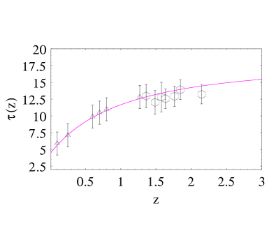
Figure 3: The observational data of the whole dataset fitted to our model, with $\mathcal{H}_{0}=1.00_{-0.07}^{+0.01}$, $s=-1.39_{-0.4}^{+0.5}$, $t_{0}=14.04\pm.08$ Gyr, and $df=3.6\pm 0.7$ Gyr. .

In the case of quartic potential we obtain $\chi_{red}^{2}=1.01$, $\mathcal{H}_{0}=1.00_{-0.05}^{+0.01}$, $\alpha_{3}=2.5_{-0.1}^{+0.5}$, $t_{0}=13.04\pm.05$ Gyr, and $df=4.2\pm 0.7$ Gyr. In the Figs.(3 and 4), the observational data are plotted vs our best fit cosmological model.

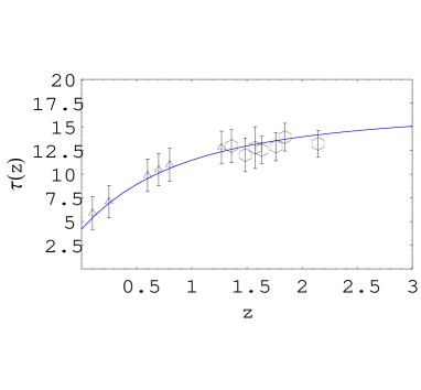
Figure 4: The observational data of the whole dataset fitted to our quartic potential model, with $\mathcal{H}_{0}=1.00_{-0.05}^{+0.01}$, $\alpha_{3}=2.5_{-0.1}^{+0.5}$, $t_{0}=13.04\pm.05$ Gyr, and $df=4.2\pm 0.7$ Gyr.

Remark: The range of values for $\mathcal{H}_{0}$ does not correspond to a variation in the physical value of $H_{0}$, which is a prior for the model. It reflects instead the scatter in the universe age.

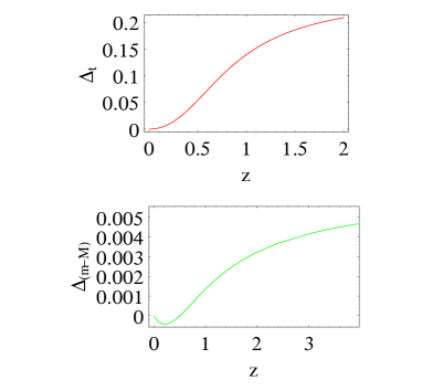
Figure 5: We compare the sensitivity to the values of the parameters in our quartic potential model in the lookback time relation and in the modulus of distance. Actually we plot the relative variation in $t(z)$ (upper diagram) and $m-M$ with respect to a variation of $\alpha_{1}$ from $3.$ to $3.5$ (the other parameters are fixed). It turns out that the $t(z)$ relation is much more sensible.

Figure 6: We compare the sensitivity of the ${dz\over dt}$ relation to the values of the parameters in the power law potential cosmological model. Actually we plot the relative variation in ${dz\over dt}$ with respect to a variation of $s$ from $-1.4$ to $-1.3$ (red line), and with respect to a variation of $\widehat{H_{0}}$ from $1$ to $.9$ (blue line), the other parameters being fixed.

4 Extending the analysis at high redshifts

Previous discussion shows that the scalar-tensor quintessence model which we are studying can be successfully constrained by cosmic clocks (clusters of galaxies) at low $(z\sim 0\div 0.5)$ and intermediate $(z\sim 1.0\div 1.5)$ redshifts. In this section we investigate its viability vs the age estimates of some high redshift objects, with a minimal stellar age of 1.8 Gyr, 3.5 Gyr and 4.0 Gyr, respectively. It is actually well known that the evolution of the universe age with redshift (${\frac{\displaystyle dt_{U}}{dz}}$) differs from a scenario to another; this means that models in which the universe is old enough to explain the total expansion age at $z=0$ may not be compatible with age estimates of high redshifts objects. This reinforces the idea that dating of objects constitutes a powerful methods to constrain the age of the universe at different stages of its evolution (Krauss & Chaboyer, (2003); Dunlop et al. (1996); Ferreras & Silk, (2003)), and the first epoch of the quasar formation can be a useful tool for discriminating among different scenarios of dark energy (Jimenez et al., (2003); Alcanitz et al., (2003)). The existence of some recently reported old high-redshift objects if of relevance here, namely LBDS 53W091, a 3.5 Gyr-old radio galaxy at $z=1.55$, LBDS 53W069, a 4 Gyr-old radio-galaxy at $z=1.43$, and APM 08279+5255, an old quasar at $z=3.91$, whose age was firstly estimated to lie in the range $2\div 3$ Gyr (Hasinger et al., (2002)), and then updated to the range $1.8\div 2.1$ Gyr (Friaça et al., 2005 ). It is clear that these objects can be used to impose more strict constraints on our model.

We take advantage for the fact that we have exact solutions, so that the redshift-time relation can be inverted. It is easily derived from Eq.(31).

Taking for granted that the universe age at any redshift must be greater than or at most equal to the age of the oldest object contained in it, we introduces the the ratio

$$\mathcal{R}\equiv{\frac{t_{z}}{t_{g}}}\geq 1,$$

as in (Alcanitz et al., (2003)), with $t_{z}$ derived from Eq. (31), and $t_{g}$ the measured age of the objects. For each extragalactic object, this inequality defines a dimensionless parameter $T_{g}=H_{o}t_{g}$. In particular, for LBDS 53W091 radio galaxy discovered by Dunlop et al. (Dunlop et al. (1996)), the lower limit for the age yields $t_{g}(z=1.55)=3.5H_{0}\$Gyr which takes values in the interval $0.21\leq T_{g}\leq 0.28$. It therefore follows that $T_{g}\geq 0.21$. Similar considerations may also be applied to the $4.0$ Gyr old galaxy at $z=1.43$, for which $T_{g}\geq 0.24$, and to the APM 08279+5255, which corresponds to $T_{g}\geq 0.131$.

Only models having an expanding age parameter larger than $T_{g}$ at the above values of redshift will be compatible with the existence of such objects.

In Figs. (7), and (8) we show the diagram of the dimensionless age parameter $T(z)=H_{0}t(z)$ as a function of the redshift for two extreme best fit values of the parameters ($s$ and $\mathcal{H}_{0}$ in the case of power law models, $\alpha_{3}$ and $\mathcal{H}_{0}$ for the quartic potential model), coming from the lookback time test. We observe that the age test turns out to be quite critical, even though such values of the parameters are fully compatible and equivalent to the $\chi^{2}$ analysis of other datasets (see Demianski et al., (2006, 2007)).

In fact, it turns out that the value $T_{g}\geq 0.131$ (Friaça et al., 2005 ) at $z=3.91$ is quite selective in both cases.

A remark is necessary at this point: the range of ages for quasar APM 08279+5255 is $1.8$ and $2$ Gyr. It is required for models from $10^{11}$ M_⊙ to $10^{12}$ M_⊙ in order to reach the metalicity Fe/O=$2.5\times$ solar unit (for details see Friaça et al., 2005 ).

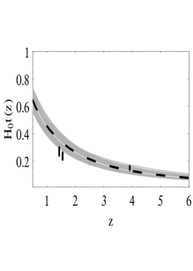
Figure 7: The dashed line indicates $T(z)=H_{0}t(z)$ according to the best fit values of Sec. IV. for the power law potential model. The shadowed region covers the allowed ranges coming from lookback time tests. The vertical lines give the lowest ages $T_{g}$of the considered objects for the allowed range of $h=(0.64\div 0.80)$. The figures reported in the text correspond to $h=0.64$, i.e. the lowest edges of the lines.For the first two objects, there is full agreement with the requirement $T>T_{g}$. The third age is marginally compatible, likely due to systematics in evaluating the age-metalicity relation.

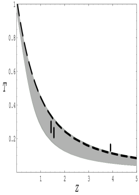
Figure 8: The same than in Fig.(8) for the quartic potentail model

5 Discussion and Conclusions

Cosmological models can be constrained not only using distance indicators but also cosmic clocks, once efficient methods are developed to estimate the age of distant objects. Among these, the relations between lookback time and redshift $z$ are particularly useful to discriminate among the huge class of dark energy models which have been recently developed to explain the observed present day accelerated behaviour of cosmic flow. In a near future, beside distance measurements, time measurements could greatly contribute to achieve a final cosmological model constraining the main cosmological parameters.

In this context, it is of fundamental importance to obtain valid cosmic clocks at low, intermediate and high redshifts in order to fit, in principle, a model at every epoch. In this case, degeneracies are removed and the reliability of the model can be proved.

In this paper, we have tested a non minimally coupled scalar-tensor quintessence model, characterised by quartic self-interacting potential, using, as cosmic clocks, cluster of galaxies at low and intermediate redshifts, two old radio galaxies at high redshift, and a very far quasar. The results are comfortable since the model seems to work in all the regimes considered. However, to be completely reliable, the dataset should be further enlarged and the method considered also for other time indicators.

The main feature of this approach is the fact that cosmic clocks are completely independent of each other, so that, in principle, it is possible to avoid biases due to primary, secondary and so on indicators, as in cosmic ladder method. In that case, every rung of the ladder is affected by the errors of former ones and it affects the successive ones. By using cosmic clocks, this shortcoming can be, in principle, avoided, since indicators are, by definition, independent. In fact, we have used different methods to test the model at low and high redshift with different indicators, which seem to confirm independently the proposed dark energy model.

Another comment is due at this point. Having normalized the Hubble parameter at present epoch, assuming $\mathcal{H}_{0}=H(1)$, we do not need, in principle, priors on such a parameter, since we are using an exact solution. In other words, we can check the validity of the model by selecting reliable cosmic clocks only. Another advantage of such a choice is that one has to handle only small numbers of parameters in numerical computations.

Appendix A The lookback time method

In order to use the age measurements of a given cosmic clock to get cosmological constraints, let us consider an object $i$ at redshift $z$ and let $t_{i}(z)$ be its age defined as the difference between the age of the universe at the formation redshift $z_{F}$, and at $z$:

$$t_{i}(z)=t_{L}(z_{F})-t_{L}(z).$$ (66)

If one is able to to estimate the ages $\{t_{i}\}$ for $i=1,2,\ldots,N$ of $N$ objects, we can estimate the lookback time $t_{L}^{obs}(z_{i})$ as

$$t_{L}^{obs}(z_{i}) =t_{L}(z_{F})-t_{i}(z)$$

$$=t_{0}^{obs}-t_{i}(z)-df\ ,$$ (67)

where $t_{0}^{obs}$ is the age of the universe (which in our units is set to 1), while the bias (delay factor) can be defined as :

$$df=t_{0}^{obs}-t_{L}(z_{F})\ .$$ (68)

The delay factor is introduced to take into account our ignorance of the formation redshift $z_{F}$ of the object. Actually, to estimate $z_{F}$, one should use Eq.(66), assuming a background cosmological model. Since our aim is to constrain the background cosmological model, it is clear that we cannot infer $z_{F}$ from the measured age, so that this quantity is a priori undetermined. Moreover we rely that it can take into account also the effect of the $G_{eff}$ variation on the age estimations, because the expected magnitude of such an effect. In principle, $df$ should be different for each object in the sample unless there is a theoretical reason to assume the same redshift at the formation of all the objects. However, we can realistically assume that $df$ is the same for all the homologous objects of a given dataset (in the range of the errors), and we consider $df$ rather than $z_{F}$ as the unknown parameter to be determined from the data.

We may then define a merit function  :

$$\chi_{lt}^{2}=\displaystyle{\frac{1}{N-N_{p}+1}}\left\{\left[\frac{t_{0}^{theor}(\mathbf{p})-t_{0}^{obs}}{\sigma_{t_{0}^{obs}}}\right]^{2}+\sum_{i=1}^{N}{\left[\frac{t_{L}^{theor}(z_{i},\mathbf{p})-t_{L}^{obs}(z_{i})}{\sqrt{\sigma_{i}^{2}+\sigma_{t}^{2}}}\right]^{2}}\right\},$$

where $N_{p}$ is the number of parameters of our model, $\sigma_{t}$, $\sigma_{i}$ are the uncertainties on $t_{0}^{obs}$ and $t_{L}^{obs}(z_{i})$. Here the superscript theor denotes the predicted values of a given quantity.

In principle, such a method can work efficiently to discriminate between the various cosmological models. However, the main difficulty is due to the lack of available data which leads to large uncertainties on the estimated parameters. In order to partially alleviate this problem, we can add further constraints on the model by using priors; for example choosing a Gaussian prior on the Hubble constant allows us to redefining the likelihood function as

$${\mathcal{L}}(\mathbf{p})\propto{\mathcal{L}}_{lt}(\mathbf{p})\exp{\left[-\frac{1}{2}\left(\frac{h-h^{obs}}{\sigma_{h}}\right)^{2}\right]}\propto\exp{[-\chi^{2}(\mathbf{p})/2],}$$ (69)

where we have absorbed $df$ to the set of parameters $\mathbf{p}$ and have defined :

$$\chi^{2}=\chi_{lt}^{2}+\left(\frac{h-h^{obs}}{\sigma_{h}}\right)^{2}$$ (70)

with $h^{obs}$ the estimated value of $h$ and $\sigma_{h}$ its uncertainty. We use the HST Key project results (Freedman et al., (2001)) setting $(h,\sigma_{h})=(0.72,0.08)$. Note that this estimate is independent of the cosmological model since it has been obtained from local distance ladder methods.

The best fit model parameters $\mathbf{p}$ may be obtained by maximizing ${\mathcal{L}}(\mathbf{p})$ which is equivalent to minimize the $\chi^{2}$ defined in Eq.(70). It is worth stressing that such a function should not be considered as a statistical $\chi^{2}$ in the sense that it is not forced to be of order 1 for the best fit model to be considered as a successful fit. Actually, such an interpretation is not possible since the errors on the measured quantities (both $t_{i}$ and $t_{0}$) are not Gaussian distributed. Moreover, there are uncontrolled systematic uncertainties that may also dominate the error budget. Moreover, there are uncontrolled systematic uncertainties that may also dominate the error budget. Nevertheless, a qualitative comparison of different models may be obtained by comparing the values of this pseudo $\chi^{2}$, even if this should not be considered as definitive evidence against a given model.

Given that we have more than one parameter, we obtain the best fit value of each single parameter $p_{i}$ as the value which maximizes the marginalized likelihood for that parameter, defined as :

$${\mathcal{L}}_{p_{i}}\propto\int{dp_{1}\ldots\int{dp_{i-1}\int{dp_{i+1}\ldots\int{dp_{n}\ {\mathcal{L}}(\mathbf{p})}}}}\ .$$ (71)

After having normalized the marginalized likelihood to 1 at maximum, we compute the $1\sigma$ and $2\sigma$ confidence limits (CL) on that parameter by solving ${\mathcal{L}}_{p_{i}}=\exp{(-0.5)}$ and ${\mathcal{L}}_{p_{i}}=\exp{(-2)}$ respectively.

References

- Andreon, (2003) S. Andreon, 2003, A&A, 409, 37.
- Clifton et al., (2004) T. Clifton, D. F. Mota, and J. D. Barrow, 2004, Mon.Not.Roy.Astron.Soc. 358, 601
- Acquaviva et al., (2005) Acquaviva V., & al., 2005, Phys.Rev. D 71 104025
- Perlmutter et al., (1997) Perlmutter S. et al., 1997, ApJ, 483, 565
- Demianski et al., (1991) Demianski M. et al., 1991, Phys.Rev.D, 44, 3136
- Perlmutter et al., (1999) Perlmutter S. et al., 1999, ApJ, 517, 565
- Riess et al., (1998) Riess et al., 1998, AJ, 116, 1009
- Riess, (2000) Riess, A.G., 2000, PASP, 112, 1284
- Steinhardt et al, (1999) P.J. Steinhardt, L. Wang, and I. Zlatev, Phys. Rev. D 59, 123504 (1999).
- Rubano et al., (2004) Rubano C., Scudellaro P., Piedipalumbo E., Capozziello S., Capone M., 2004, Phys. Rev. D, 69, 103510
- Amendola, (1999) Amendola L., 1999, Phys. Rev. D 60, 043501
- Boisseau et al., (2000) Boisseau B., Esposito-Farese G., Polarski D., & Starobinsky A..A., 2000, Phys. Rev. Lett., 85 2236
- Torres, (2002) Torres D.F., Phys. Rev. D, 2002, 66, 043522
- Faraoni, (2000) Faraoni V., 2000 Phys.Rev. D, 62, 023504
- Caldwell et al., (2003) Caldwell R.R., Kamionkowski M., Weinberg N.N., 2003, Phys.Rev.Lett., 91, 071301
- Hu, (2005) Hu W., 2005, Phys. Rev. D, 71, 047301
- Vikman, (2005) Vikman A., 2005, Phys. Rev. D, 71, 023515
- Nojiri & Odintsov, (2005) S. Nojiri, S.D. Odintsov, hep-th/0506212 (2005);
- Dvali et al., (2000) G.R. Dvali, G. Gabadadze, M. Porrati, Phys. Lett. B, 485, 208, 2000;
- Chiba, (1999) Chiba T., 1999, Phys. Rev. D 60, 083508
- Capozziello, (2002) S. Capozziello, Int. J. Mod. Phys. D, 11, 483, 2002
- Capozziello et al., (2003) S. Capozziello, V.F. Cardone, S. Carloni, A. Troisi, Int. J. Mod. Phys. D, 12, 1969, 2003
- Gaztañaga et al., (2001) Gaztañaga E., Garcia-Berro E., Isern J., Bravo E., & Dominguez, 2001, Phys. Rev. D, 1
- Dantas et al., (2007) Dantas M.A., et al., astro-ph/0607060, in press on A&A
- Nojiri & Odintsov, (2003) S. Nojiri, S.D. Odintsov, Phys. Lett. B, 576, 5, 2003
- Vollick, (2003) D.N. Vollick, Phys. Rev. 68, 063510, 2003
- Meng & Wang, (2003) X.H. Meng, P. Wang, Class. Quant. Grav., 20, 4949, 2003
- Flanagan, (2004) E.E. Flanagan, Class. Quant. Grav., 21, 417, 2004
- Allemandi et al., (2004) G. Allemandi, A. Borowiec, M. Francaviglia, Phys. Rev. D, 70, 043524, 2004
- Demianski et al., (2005) Demianski M., Piedipalumbo E., Rubano C., Tortora C., 2005, A&A, 431, 27
- Demianski et al., (2006) Demianski M., Piedipalumbo E., Rubano C., Tortora C., 2006, A&A, 454, 55-66
- Demianski et al., (2007) Demianski M., Piedipalumbo E., Rubano C., Tortora C., submitted to A&A
- Fujii, (2000) Fujii Y., 2000, Phys. Rev. D, 62, 044011
- Spergel et al., (2003) Spergel D.N., et al., 2003, ApJ, 148, 175
- Krauss & Chaboyer, (2003) Krauss L. M., Chaboyer B., 2003, Science, 299, 65
- Jimenez & Loeb, (2002) R. Jimenez, A. Loeb, ApJ, 573, 37, 2002
- Jimenez et al., (2003) R. Jimenez, L. Verde, T Treu, D. Stern, 2003, ApJ, 593, 622
- Lima & Alcaniz, (2000) Lima J. A. S. & Alcaniz J. S., 2000, MNRAS, 317, 893
- Alcanitz et al., (2003) Alcanitz J.S., Lima J.A.S., Cunha J.H., 2003, MNRAS, 340, 39
- Capozziello & de Ritis, (1994) Capozziello S. & de Ritis R, Class. Quantum Grav. 11, 107, 1994.
- Capozziello et al, (1996) S. Capozziello, R. de Ritis, C. Rubano, and P. Scudellaro, Riv. del Nuovo Cimento 19, vol. 4 (1996).
- Capozziello et al., (2004) Capozziello S., Cardone V.F., Funaro M., Andreon S., Phys.Rev. D, 2004, 70 123501
- Damour & Esposito-Farese, (1993) Damour T., Esposito-Farese G., Phys. Rev. Lett. 70, 2220 (1993)
- Dalal et al., (2001) N. Dalal, K. Abazajian, E. Jenkins, A.V. Manohar, Phys. Rev. Lett., 87, 141302, 2001
- Ferreras et al., (2003) Ferreras I., Melchiorri A., Tocchini Valentini D., MNRAS, 344, 257, 2003
- Andreon et al, (2004) Andreon S. et al., MNRAS, 353, 353, 2004; S. Andreon, C. Lobo, A. Iovino, MNRAS, 349, 889, 2004.
- Ellis & Madsen, (1991) Ellis G.F.R. and Madsen M.S., Class. Quant. Grav. 8, 667, 1991.
- Amendola et al., (1994) Amendola L., Khalatnikov I.M., Litterio M., and Occhionero F., Phys. Rev., D 49, 1881, 1994.
- Kamenshchik et al., (1995) Kamenshchik A. Yu., Khalatnikov I.M., Toporensky A.V., Phys. Lett., B 357, 36, 1995.
- Capozziello & de Ritis, (1993) Capozziello S. & de Ritis R., Phys. Lett. A 177 , 1, 1993.
- Freedman et al., (2001) Freedman W.L., et al., ApJ, 553, 47, 2001.
- Worthey, (1992) Worthey G., Ph.D. Thesis California Univ., Santa Cruz, 1992
- Bower et al., (1998) Bower R.G., Lucey J.R., Ellis R.S.,1998 MNRAS, 254, 601
- Dunlop et al. (1996) Dunlop J., et al., 1996, Nature, 381, 581
- Perrotta et al., (2000) Perrotta F., Baccigalupi C., and Matarrese S., 2000, Phys.Rev. D 61 023507
- Ferreras & Silk, (2003) Ferreras I., Silk J., 2003, MNRAS, 344, 455
- Hasinger et al., (2002) Hasinger G., Scharte N., Komossa S., 2002, ApJ, 573 L77
- (58) Friaça A., Alcaniz J.S., Lima J. A. S., astro-ph/0504031 (2005).
- Riazuelo & Uzan, (2002) Riazuelo A., & Uzan J.- P., 2002, Phys. Rev. D, 66, 023525
- Saini et al, (2003) Saini T. D., Padmanabhan T., Bridle S., 2003, Mon.Not.Roy.Astron.Soc., 343, 533
- Uzan, (1998) Uzan J.Ph., 1998, Phys. Rev D, 59, 123510
- Schimd et al., (2005) Schimd C., Uzan J. P., and Riazuelo A., 2005, Phys. Rev. D 71, 083512
- Will, (1993) C.M. Will, Theory and Experiments in Gravitational Physics (1993) Cambridge Univ. Press, Cambridge.