Mott–Hubbard Transition and Anderson Localization: Generalized Dynamical Mean-Field Theory Approach

Abstract

Density of states, dynamic (optical) conductivity and phase diagram of strongly correlated and strongly disordered paramagnetic Anderson–Hubbard model are analyzed within the generalized dynamical mean field theory (DMFT+$\Sigma$ approximation). Strong correlations are accounted by DMFT, while disorder is taken into account via the appropriate generalization of self-consistent theory of localization. The DMFT effective single impurity problem is solved by numerical renormalization group (NRG) and we consider the three-dimensional system with semi-elliptic density of states. Correlated metal, Mott insulator and correlated Anderson insulator phases are identified via the evolution of density of states and dynamic conductivity, demonstrating both Mott-Hubbard and Anderson metal-insulator transition and allowing the construction of complete zero-temperature phase diagram of Anderson–Hubbard model. Rather unusual is the possibility of disorder induced Mott insulator to metal transition.

I Introduction

The importance of the electronic interaction and randomness for the properties of condensed matter is well known Lee85 . Coulomb correlations and disorder are both driving forces of metal–insulator transitions (MITs) connected with the localization and delocalization of particles. In particular, the Mott–Hubbard MIT is caused by the electronic repulsion Mott90 , while Anderson MIT is due to random scattering of non–interacting particles Anderson58 . Actually, disorder and interaction effects are known to compete in many subtle ways Lee85 ; ma and this problem becomes much more complicated in the case of strong electron correlations and strong disorder, determining the physical mechanisms of Mott–Anderson MIT Lee85 .

The cornerstone of the modern theory of strongly correlated systems is the dynamical mean–field theory (DMFT) MetzVoll89 ; vollha93 ; pruschke ; georges96 , constituting a non–perturbative theoretical framework for the investigation of correlated lattice electrons with a local interaction. In this approach the effect of local disorder can be taken into account through the standard average density of states (DOS) ulmke95 in the absence of interactions, leading to the well known coherent potential approximation vlaming92 , which does not describe the physics of Anderson localization. To overcome this deficiency Dobrosavljević and Kotliar Dobrosavljevic97 formulated a variant of the DMFT where the geometrically averaged local DOS was computed from the solutions of the self–consistent stochastic DMFT equations. Subsequently, Dobrosavljević et al. Dobrosavljevic03 incorporated the geometrically averaged local DOS into the self–consistency cycle and derived a mean–field theory of Anderson localization which reproduced many of the expected features of the disorder–driven MIT for non–interacting electrons. This approach was extended by Byczuk et al. BV to include Hubbard correlations via DMFT, which lead to highly non trivial phase diagram of Anderson–Hubbard model with correlated metal, Mott insulator and correlated Anderson insulator phases. The main deficiency of these approaches, however, is inability to calculate directly measurable physical properties, such as conductivity, which is of major importance and defines MIT itself.

At the same time the well developed approach of self–consistent theory of Anderson localization, based on solving the equations for the generalized diffusion coefficient, demonstrated its efficiency in non–interacting case long ago VW ; WV ; MS ; MS86 ; VW92 ; Diagr and some attempts to include interaction effects within this approach were also undertaken with some promising results MS86 ; KSS . However, up to now there were no attempts to incorporate this approach to the modern theory of strongly correlated electronic systems. Here we undertake such research, studying both Mott–Hubbard and Anderson MITs via direct calculations of both the average DOS and dynamic (optical) conductivity.

Our approach is based on recently proposed generalized DMFT+$\Sigma$ approximation JTL05 ; PRB05 ; FNT06 ; PRB07 , which on the one hand retains the single-impurity description of the DMFT, with a proper account for local Hubbard–like correlations and the possibility to use impurity solvers like NRGNRG ; BPH ; Bull , while on the other hand, allows one to include additional (either local or non-local) interactions (fluctuations) on a non-perturbative model basis.

Within this approach we have already studied both single- and two-particle properties, of two–dimensional Hubbard model, concentrating mainly on the problem of pseudogap formation in the density of states of the quasiparticle band in both correlated metals and doped Mott insulators, with an application to superconducting cuprates. We analyzed the evolution of non–Fermi liquid like spectral density and ARPES spectra PRB05 , “destruction” of Fermi surfaces and formation of Fermi “arcs” JTL05 , as well as pseudogap anomalies of optical conductivity PRB07 . Briefly we also considered impurity scattering effects FNT06 .

In this paper we apply our DMFT+$\Sigma$ approach for calculations of the density of states, dynamic conductivity and phase diagram of strongly correlated and strongly disordered three–dimensional paramagnetic Anderson–Hubbard model. Strong correlations are again accounted by DMFT, while disorder is taken into account via the appropriate generalization of self-consistent theory of localization.

The paper is organized as follows: In section II we present a short description of our generalized DMFT+$\Sigma$ approximation with application to disordered Hubbard model. In section III we present basic DMFT+$\Sigma$ expressions for dynamic (optical) conductivity and formulate appropriate self–consistent equations for the generalized diffusion coefficient. Computational details and results for density of states and dynamic conductivity are given in section IV, where we also analyze the phase diagram of strongly disordered Hubbard model, following from our approach. The paper is ended with a short summary section V including a discussion of some related problems.

II Basics of DMFT+$\Sigma$ approach

Our aim is to consider non–magnetic disordered Anderson–Hubbard model (mainly) at half–filling for arbitrary interaction and disorder strengths. Mott–Hubbard and Anderson MITs will be investigated on an equal footing. The Hamiltonian of the model under study is written as:

$$H=-t\sum_{\langle ij\rangle\sigma}a_{i\sigma}^{\dagger}a_{j\sigma}+\sum_{i\sigma}\epsilon_{i}n_{i\sigma}+U\sum_{i}n_{i\uparrow}n_{i\downarrow},$$ (1)

where $t>0$ is the amplitude for hopping between nearest neighbors, $U$ is the on–site repulsion, $n_{i\sigma}=a_{i\sigma}^{\dagger}a_{i\sigma}^{{\phantom{\dagger}}}$ is the local electron number operator, $a_{i\sigma}$ ($a_{i\sigma}^{\dagger}$) is the annihilation (creation) operator of an electron with spin $\sigma$, and the local ionic energies $\epsilon_{i}$ at different lattice sites are considered to be independent random variables. To simplify diagrammatics in the following we assume Gaussian probability distribution for $\epsilon_{i}$:

$$\mathcal{P}(\epsilon_{i})=\frac{1}{\sqrt{2\pi}\Delta}\exp\left(-\frac{\epsilon_{i}^{2}}{2\Delta^{2}}\right)$$ (2)

Here the parameter $\Delta$ is just a measure of disorder strength, and Gaussian (“white” noise) random field of energy level $\epsilon_{i}$ at lattice cites produces “impurity” scattering, leading to the standard diagram technique for calculation on the averaged Green’s functions Diagr .

DMDF+$\Sigma$ approach was initially proposed JTL05 ; PRB05 ; FNT06 as a simple method to include non–local fluctuations, essentially of arbitrary nature, to the standard DMFT. In fact it can be used to include into DMFT any additional interaction in the following way. Working at finite temperatures $T$ we write down Matsubara “time” Fourier transformed single-particle Green function of the Hubbard model as:

$$G(i\varepsilon,{\bf p})=\frac{1}{i\varepsilon+\mu-\epsilon({\bf p})-\Sigma(i\varepsilon)-\Sigma_{\bf p}(i\varepsilon_{n})},\varepsilon=\pi T(2n+1),$$ (3)

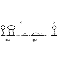
Figure 1: Typical “skeleton” diagrams for the self–energy in the DMFT+$\Sigma$ approach. The first two terms are examples of DMFT self–energy diagrams; the middle two diagrams show contributions due to random impurity scattering represented as dashed lines. The last diagram (b) is an example of neglected diagram leading to interference between the local Hubbard interaction and impurity scattering.

where $\epsilon({\bf p})$ is the single particle spectrum, corresponding to free part of (1), $\mu$ is chemical potential fixed by electron concentration, and $\Sigma(i\varepsilon)$ is the local contribution to self–energy due to Hubbard interaction, of DMFT type (surviving in the limit of spatial dimensionality $d\to\infty$), while $\Sigma_{\bf p}(i\varepsilon)$ is some additional (in general momentum dependent) self–energy part. This last contribution can be due e.g. to electron interactions with some “additional” collective modes or order parameter fluctuations within the Hubbard model itself. But actually it can be due to any other interactions (fluctuations) outside the standard Hubbard model, e.g. due to phonons or to random impurity scattering, when it is in fact local (momentum independent). The last interaction will be our main interest in the present paper. Basic assumption here is the neglect of all interference processes of the local Hubbard interaction and “external” contributions due to these additional scatterings (non-crossing approximation for appropriate diagrams) PRB05 , as illustrated by diagrams in Fig. 1.

The self–consistency equations of generalized DMFT+$\Sigma$ approach are formulated as follows JTL05 ; PRB05 :

1. Start with some initial guess of local self–energy $\Sigma(i\varepsilon)$, e.g. $\Sigma(i\varepsilon)=0$.

2. Construct $\Sigma_{\bf p}(i\varepsilon)$ within some (approximate) scheme, taking into account interactions with “external” interaction (impurity scattering in our case) which in general can depend on $\Sigma(i\omega)$ and $\mu$.

3. Calculate the local Green function

   $$G_{ii}(i\varepsilon)=\frac{1}{N}\sum_{\bf p}\frac{1}{i\varepsilon+\mu-\epsilon({\bf p})-\Sigma(i\varepsilon)-\Sigma_{\bf p}(i\varepsilon)}.$$ (4)

4. Define the “Weiss field”

   $${\cal G}^{-1}_{0}(i\varepsilon)=\Sigma(i\varepsilon)+G^{-1}_{ii}(i\varepsilon).$$ (5)

5. Using some “impurity solver” calculate the single-particle Green function $G_{d}(i\varepsilon)$ for the effective Anderson impurity problem, placed at lattice site $i$ and defined by effective action which is written, in obvious notations, as:

   $$S_{\text{eff}}=-\int_{0}^{\beta}d\tau_{1}\int_{0}^{\beta}d\tau_{2}c_{i\sigma}(\tau_{1}){\cal G}^{-1}_{0}(\tau_{1}-\tau_{2})c^{+}_{i\sigma}(\tau_{2})$$

   $$+\int_{0}^{\beta}d\tau Un_{i\uparrow}(\tau)n_{i\downarrow}(\tau).$$ (6)

   Actually, in the following, for the “impurity solver” we use NRG NRG ; BPH ; Bull , which allows us to deal also with real frequencies, thus avoiding the complicated problem of analytical continuation from Matsubara frequencies.

6. Define a new local self–energy

   $$\Sigma(i\omega)={\cal G}^{-1}_{0}(i\omega)-G^{-1}_{d}(i\omega).$$ (7)

7. Using this self–energy as “initial” one in step 1, continue the procedure until (and if) convergency is reached to obtain

   $$G_{ii}(i\varepsilon)=G_{d}(i\varepsilon).$$ (8)

Eventually, we get the desired Green function in the form of (3), where $\Sigma(i\varepsilon)$ and $\Sigma_{\bf p}(i\varepsilon)$ are those appearing at the end of our iteration procedure.

For $\Sigma_{\bf p}(i\varepsilon_{n})$ of the random impurity problem we shall use the simplest possible one–loop contribution, given by the third diagram of Fig. 1 (a), neglecting “crossing” diagrams like the fourth one in Fig. 1 (a), i.e. just the self–consistent Born approximation Diagr , which in the case of Gaussian disorder (2) leads to the usual expression:

$$\Sigma_{\bf p}(i\varepsilon)=\Delta^{2}\sum_{\bf p}G(i\varepsilon,{\bf p})\equiv\Sigma_{imp}(i\varepsilon)$$ (9)

which is actually ${\bf p}$-independent (local).

III Dynamic conductivity in DMFT+$\Sigma$ approach

III.1 Basic expressions for optical conductivity

Physically it is clear that calculations of dynamic conductivity are the most direct way to study MITs, as its frequency dependence along with static value at zero frequency of an external field allows the clear distinction between metallic and insulating phases (at zero temperature $T=0$).

To calculate dynamic conductivity we use the general expression relating it to retarded density–density correlation function $\chi^{R}(\omega,{\bf q})$ VW ; Diagr :

$$\sigma(\omega)=-\lim_{q\to 0}\frac{ie^{2}\omega}{q^{2}}\chi^{R}(\omega,{\bf q}),$$ (10)

where $e$ is electronic charge.

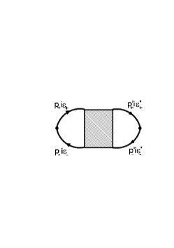
Figure 2: Full polarization loop with vertex part, describing all interactions and impurity scatterings in particle–hole channel. The loop without vertex corrections is included implicitly. Here ${\bf p}_{\pm}={\bf p}\pm\frac{\bf q}{2}$, $\varepsilon_{\pm}=\varepsilon\pm\frac{\omega}{2}$.

Next we briefly follow the derivation presented in detail in Ref. PRB07 for the pseudogap problem, with necessary modifications for the present case. Consider full polarization loop graph in Matsubara representation shown in Fig. 2, which is conveniently (with explicit frequency summation) written as:

$$\Phi(i\omega,{\bf q})=\sum_{\varepsilon\varepsilon^{\prime}}\Phi_{i\varepsilon i\varepsilon^{\prime}}(i\omega,{\bf q})\equiv\sum_{\varepsilon}\Phi_{i\varepsilon}(i\omega,{\bf q})$$ (11)

and contains all possible interactions of our model, described by the full shaded vertex part. Actually we implicitly assume here that simple loop contribution without vertex corrections is also included in Fig. 2, which shortens further diagrammatic expressions PRB07 . Retarded density–density correlation function is determined by appropriate analytic continuation of this loop and can be written asVW :

$$\chi^{R}(\omega,{\bf q})=\int_{-\infty}^{\infty}\frac{d\varepsilon}{2\pi i}\left\{\left[f(\varepsilon_{+})-f(\varepsilon_{-})\right]\Phi_{\varepsilon}^{RA}({\bf q},\omega)\right.$$

$$\left.+f(\varepsilon_{-})\Phi_{\varepsilon}^{RR}({\bf q},\omega)-f(\varepsilon_{+})\Phi_{\varepsilon}^{AA}({\bf q},\omega)\right\},$$ (12)

where $f(\varepsilon)$ – Fermi distribution, $\varepsilon_{\pm}=\varepsilon\pm\frac{\omega}{2}$, while two–particle loops $\Phi_{\varepsilon}^{RA}({\bf q},\omega)$, $\Phi_{\varepsilon}^{RR}({\bf q},\omega)$, $\Phi_{\varepsilon}^{AA}({\bf q},\omega)$ are determined by appropriate analytic continuations $(i\varepsilon+i\omega\to\varepsilon+\omega+i\delta,i\varepsilon\to\varepsilon\pm i\delta,\delta\to+0)$ in (11). Then we can write dynamic (optical) conductivity as:

$$\sigma(\omega)=\lim_{q\to 0}\left(-\frac{e^{2}\omega}{2\pi q^{2}}\right)\int_{-\infty}^{\infty}d\varepsilon$$

$$\left\{\left[f(\varepsilon_{+})-f(\varepsilon_{-})\right]\left[\Phi_{\varepsilon}^{RA}({\bf q},\omega)-\Phi_{\varepsilon}^{RA}(0,\omega)\right]\right.$$

$$\left.+f(\varepsilon_{-})\left[\Phi_{\varepsilon}^{RR}({\bf q},\omega)-\Phi_{\varepsilon}^{RR}(0,\omega)\right]\right.$$

$$\left.-f(\varepsilon_{+})\left[\Phi_{\varepsilon}^{AA}({\bf q},\omega)-\Phi_{\varepsilon}^{AA}(0,\omega)\right]\right\},$$ (13)

where the total contribution of additional terms with zero $q$ can be shown (with the use of general Ward identities) to be zero.

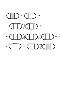
Figure 3: Bethe–Salpeter equation for polarization loop in DMFT+$\Sigma$ approach. Circle represents irreducible vertex part in particle–hole channel of DMFT, which contains only local Hubbard interactions. Unshaded rectangular vertex represents corrections from impurity scattering only, implicitly including the case free particle–hole propagation.

To calculate $\Phi_{i\varepsilon i\varepsilon^{\prime}}(i\omega,{\bf q})$, entering the sum over Matsubara frequencies in (11), in DMFT+$\Sigma$ approximation, which neglects interference between local Hubbard interaction and impurity scatterings, we can write down Bethe–Salpeter equation, shown diagrammatically in Fig. 3, where we introduce irreducible (local) vertex $U_{i\varepsilon i\varepsilon^{\prime}}(i\omega)$ of DMFT and “rectangular” vertex, containing all interactions with impurities. Analytically this equation can be written as:

$$\Phi_{i\varepsilon i\varepsilon^{\prime}}(i\omega,{\bf q})=\Phi^{0}_{i\varepsilon}(i\omega,{\bf q})\delta_{\varepsilon\varepsilon^{\prime}}$$

$$+\Phi^{0}_{i\varepsilon}(i\omega,{\bf q})\sum_{\varepsilon^{\prime\prime}}U_{i\varepsilon i\varepsilon^{\prime\prime}}(i\omega)\Phi_{i\varepsilon^{\prime\prime}i\varepsilon^{\prime}}(i\omega,{\bf q}),$$ (14)

where $\Phi^{0}_{i\varepsilon}(i\omega,{\bf q})$ is the desired function calculated neglecting vertex corrections due to Hubbard interaction (but taking into account all interactions due to impurity scattering). Note that all $q$-dependence here is determined by $\Phi^{0}_{i\varepsilon}(i\omega,{\bf q})$ as the vertex $U_{i\varepsilon i\varepsilon^{\prime}}(i\omega)$ is local and $q$-independent.

As we noted in Ref. PRB07 , it is clear from (13) that calculation of conductivity requires only the knowledge of $q^{2}$-contribution to $\Phi(i\omega,{\bf q})$. This can be easily found in the following way. First of all, note that all the loops in (14) contain $q$-dependence starting from terms of the order of $q^{2}$. Then we can take an arbitrary loop (crossection) in the expansion of (14) (see Fig. 3), calculating it up to terms of the order of $q^{2}$, and make resummation of all contributions to the right and to the left from this crossection, putting $q=0$ in all these graphs. This is equivalent to simple $q^{2}$-differentiation of the expanded version of Eq. (14). This procedure immediately leads to the following relation for $q^{2}$-contribution to (11):

$$\phi(i\omega)\equiv\lim_{q\to 0}\frac{\Phi(i\omega,{\bf q})-\Phi(i\omega,0)}{q^{2}}=\sum_{\varepsilon}\gamma^{2}_{i\varepsilon}(i\omega,{\bf q}=0)\phi^{0}_{i\varepsilon}(i\omega)$$ (15)

where

$$\phi^{0}_{i\varepsilon}(i\omega)\equiv\lim_{q\to 0}\frac{\Phi^{0}_{i\varepsilon}(i\omega,{\bf q})-\Phi^{0}_{i\varepsilon}(i\omega,0)}{q^{2}}$$ (16)

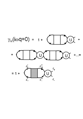
Figure 4: Effective vertex $\gamma_{i\varepsilon}(i\omega,{\bf q}=0)$ used in calculations of conductivity.

where $\Phi^{0}_{i\varepsilon}(i\omega,{\bf q})$ contains vertex corrections only due to impurity scattering, while one-particle Green’s functions entering it are taken with self-energies due to both impurity scattering and local DMFT-like interaction, like in Eq. (3). The vertex $\gamma_{i\varepsilon}(i\omega,{\bf q}=0)$ is determined diagrammatically as shown in Fig. 4, or analytically:

$$\gamma_{i\varepsilon}(i\omega,{\bf q}=0)=1+\sum_{\varepsilon^{\prime}\varepsilon^{\prime\prime}}U_{i\varepsilon i\varepsilon^{\prime\prime}}(i\omega)\Phi_{i\varepsilon^{\prime\prime}i\varepsilon^{\prime}}(i\omega,{\bf q}=0).$$ (17)

Now using Bethe–Salpeter equation (14) we can write explicitly:

$$\gamma_{i\varepsilon}(i\omega,{\bf q}=0)=1+$$

$$+\sum_{\varepsilon^{\prime}}\frac{\Phi_{i\varepsilon i\varepsilon^{\prime}}(i\omega,{\bf q}=0)-\Phi^{0}_{i\varepsilon}(i\omega,{\bf q}=0)}{\Phi^{0}_{i\varepsilon}(i\omega,{\bf q}=0)}=$$

$$=\frac{\sum_{\varepsilon^{\prime}}\Phi_{i\varepsilon i\varepsilon^{\prime}}(i\omega,{\bf q}=0)}{\Phi^{0}_{i\varepsilon}(i\omega,{\bf q}=0)}.$$ (18)

For ${\bf q}=0$ we have the following Ward identity, which can be obtained by direct generalization of the proof given in VW ; Mig (see details in Appendix of Ref. PRB07 ):

$$(-i\omega)\Phi_{i\varepsilon}(i\omega,{\bf q}=0)=(-i\omega)\sum_{\varepsilon^{\prime}}\Phi_{i\varepsilon i\varepsilon^{\prime}}(i\omega,{\bf q}=0)$$

$$=\sum_{\bf p}G(i\varepsilon+i\omega,{\bf p})-\sum_{\bf p}G(i\varepsilon,{\bf p}).$$ (19)

Denominator of (18) contains vertex corrections only from impurity scattering, while Green’s functions here are “dressed” both by impurities and local (DMFT) Hubbard interaction. Thus we may consider the loop entering the denominator as dressed by impurities only, but with “bare” Green’s functions:

$$\tilde{G}_{0}(i\varepsilon,{\bf p})=\frac{1}{i\varepsilon+\mu-\epsilon({\bf p})-\Sigma(i\varepsilon)},$$ (20)

where $\Sigma(i\varepsilon)$ is local contribution to self-energy from DMFT. For this problem we have the following Ward identity, similar to (19) (see Appendix of Ref. PRB07 ):

$$\sum_{\bf p}G(i\varepsilon+i\omega,{\bf p})-\sum_{\bf p}G(i\varepsilon,{\bf p})=$$

$$=\Phi_{i\varepsilon}^{0}(i\omega,{\bf q}=0)\left[\Sigma(i\varepsilon+i\omega)-\Sigma(i\varepsilon)-i\omega\right]\equiv$$

$$\equiv\Phi_{i\varepsilon}^{0}(i\omega,{\bf q}=0)\left[\Delta\Sigma(i\omega)-i\omega\right],$$ (21)

where we have introduced

$$\Delta\Sigma(i\omega)=\Sigma(i\varepsilon+i\omega)-\Sigma(i\varepsilon).$$ (22)

Thus, using (19), (21) in (18) we get the final expression for $\gamma_{i\varepsilon}(i\omega,{\bf q}=0)$:

$$\gamma_{i\varepsilon}(i\omega,{\bf q}=0)=1-\frac{\Delta\Sigma(i\omega)}{i\omega}.$$ (23)

Then (15) reduces to:

$$\phi(i\omega)=\sum_{\varepsilon}\phi^{0}_{i\varepsilon}(i\omega)\left[1-\frac{\Delta\Sigma(i\omega)}{i\omega}\right]^{2}.$$ (24)

Analytic continuation to real frequencies is obvious and using (15), (24) in (13) we can write the final expression for the real part of dynamic (optical) conductivity as:

$${\rm{Re}}\sigma(\omega)=\frac{e^{2}\omega}{2\pi}\int_{-\infty}^{\infty}d\varepsilon\left[f(\varepsilon_{-})-f(\varepsilon_{+})\right]$$

$${\rm{Re}}\left\{\phi^{0RA}_{\varepsilon}(\omega)\left[1-\frac{\Sigma^{R}(\varepsilon_{+})-\Sigma^{A}(\varepsilon_{-})}{\omega}\right]^{2}-\right.$$

$$\left.-\phi^{0RR}_{\varepsilon}(\omega)\left[1-\frac{\Sigma^{R}(\varepsilon_{+})-\Sigma^{R}(\varepsilon_{-})}{\omega}\right]^{2}\right\}.$$ (25)

Thus we have achieved a great simplification of our problem. To calculate dynamic conductivity in DMFT+$\Sigma$ approximation we only have to solve single–particle problem as described by DMFT+$\Sigma$ procedure above to determine self–consistent values of local self–energies $\Sigma(\varepsilon_{\pm})$, while non-trivial contribution of impurity scattering are to be included via (16), which is to be calculated in some approximation, taking into account only interaction with impurities (random scattering), but using the “bare” Green’s functions of the form (20), which include local self–energies already determined via the general DMFT+$\Sigma$ procedure. Actually (25) provides also an effective algorithm to calculate dynamic conductivity in standard DMFT (neglecting impurity scattering), as (16) is then easily calculated from a simple loop diagram, determined by two Green’s functions and free scalar vertices. As usual, there is no need to calculate vertex corrections within DMFT itself, as was proven first considering the loop with vector vertices pruschke ; georges96 . Obviously, Eq. (25) provides effective interpolation between the case of strong correlations without disorder and the case of pure disorder, without Hubbard correlations, which is of major interest to us. In the following we shall see that calculations based on Eq. (25) give a reasonable overall picture of MIT in Anderson–Hubbard model.

III.2 Self-consistent equations for generalized diffusion coefficient and conductivity

Now to calculate optical conductivity we need the knowledge of the basic block $\Phi^{0}_{i\varepsilon}(i\omega,{\bf q})$, entering (16), or, more precisely, appropriate functions analytically continued to real frequencies: $\Phi^{0RA}_{\varepsilon}(\omega,{\bf q})$ and $\Phi^{0RR}_{\varepsilon}(\omega,{\bf q})$, which in turn define $\phi^{0RA}_{\varepsilon}(\omega)$ and $\phi^{0RR}_{\varepsilon}(\omega)$ entering (25), and defined by obvious relations similar to (16):

$$\phi^{0RA}_{\varepsilon}(\omega)=\lim_{q\to 0}\frac{\Phi^{0RA}_{\varepsilon}(\omega,{\bf q})-\Phi^{0RA}_{\varepsilon}(\omega,0)}{q^{2}},$$ (26)

$$\phi^{0RR}_{\varepsilon}(\omega)=\lim_{q\to 0}\frac{\Phi^{0RR}_{\varepsilon}(\omega,{\bf q})-\Phi^{0RR}_{\varepsilon}(\omega,0)}{q^{2}}.$$ (27)

By definition we have:

$$\Phi^{0RA}_{\varepsilon}(\omega,{\bf q})=\sum_{\bf p}G^{R}(\varepsilon_{+},{\bf p_{+}})G^{A}(\varepsilon_{-},{\bf p_{-}})\times$$

$$\times\Gamma^{RA}(\varepsilon_{-},{\bf p}_{-};\varepsilon_{+},{\bf p}_{+})$$ (28)

$$\Phi^{0RR}_{\varepsilon}(\omega,{\bf q})=\sum_{\bf p}G^{R}(\varepsilon_{+},{\bf p_{+}})G^{R}(\varepsilon_{-},{\bf p_{-}})\times$$

$$\times\Gamma^{RR}(\varepsilon_{-},{\bf p}_{-};\varepsilon_{+},{\bf p}_{+}),$$ (29)

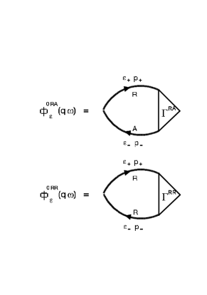
Figure 5: Diagrammatic representation of $\Phi^{0RA}_{\varepsilon}(\omega,{\bf q})$ and $\Phi^{0RR}_{\varepsilon}(\omega,{\bf q})$.

which are shown diagrammatically in Fig. 5 and ${\bf p}_{\pm}={\bf p}\pm\frac{\bf q}{2}$. Here Green’s functions $G^{R}(\varepsilon_{+},{\bf p_{+}})$ and $G^{A}(\varepsilon_{-},{\bf p_{-}})$ are defined by analytic continuation $(i\varepsilon\to\varepsilon\pm i\delta)$ of Matsubara Green’s functions (3) determined via our DMFT+$\Sigma$ algorithm (4) – (9), while vertices $\Gamma^{RA}(\varepsilon_{-},{\bf p}_{-};\varepsilon_{+},{\bf p}_{+})$ and $\Gamma^{RR}(\varepsilon_{-},{\bf p}_{-};\varepsilon_{+},{\bf p}_{+})$ contain all vertex corrections due to impurity scatterings.

The most important block $\Phi^{0RA}_{\varepsilon}(\omega,{\bf q})$ can be calculated using the basic approach of self–consistent theory of localization VW ; WV ; MS ; MS86 ; VW92 ; Diagr with appropriate extensions, taking into account the role of the local Hubbard interaction using DMFT+$\Sigma$ approach. The only important difference with the standard approach is that equations of self–consistent theory are now derived using

$$G^{R,A}(\varepsilon,{\bf p})=\frac{1}{\varepsilon+\mu-\epsilon({\bf p})-\Sigma^{R,A}(\varepsilon)-\Sigma^{R,A}_{imp}(\varepsilon)}$$ (30)

containing DMFT contributions $\Sigma^{R,A}(\varepsilon)$, not only impurity scattering contained in:

$$\Sigma_{imp}^{R,A}(\varepsilon)=\Delta^{2}\sum_{\bf p}G^{R,A}(\varepsilon,{\bf p})={\rm Re}\Sigma_{imp}(\varepsilon)\pm i\gamma(\varepsilon)$$ (31)

where $\gamma(\varepsilon)=\pi\Delta^{2}N(\varepsilon)$ and $N(\varepsilon)$ is the density of states renormalized by Hubbard interaction, accounted via DMFT+$\Sigma$ and given as usual by:

$$N(\varepsilon)=-\frac{1}{\pi}\sum_{\bf p}{\rm Im}G^{R}(\varepsilon,{\bf p})$$ (32)

Following all the usual steps of standard derivation VW ; WV ; MS ; MS86 ; VW92 ; Diagr we obtain diffusion like (at small $\omega$ and $q$) contribution to $\Phi^{0RA}_{\varepsilon}(\omega,{\bf q})$ as:

$$\Phi^{0RA}_{\varepsilon}({\bf q},\tilde{\omega})=\frac{2\pi iN(\varepsilon)}{\tilde{\omega}+iD(\omega)q^{2}}$$ (33)

where important difference with the single–particle case is contained in

$$\tilde{\omega}=\varepsilon_{+}-\varepsilon_{-}-\Sigma^{R}(\varepsilon_{+})+\Sigma^{A}(\varepsilon_{-})=$$

$$=\omega-\Sigma^{R}(\varepsilon_{+})+\Sigma^{A}(\varepsilon_{-})\equiv\omega-\Delta\Sigma^{RA}(\omega)$$ (34)

which replaces the usual $\omega$ term in the denominator of the standard expression for $\Phi^{0RA}_{\varepsilon}(\omega,{\bf q})$. On general grounds it is clear that in metallic phase for $\omega\to 0$ we have $\Delta\Sigma^{RA}(\omega=0)=2{\rm iIm}\Sigma(\varepsilon)\sim Max\{T^{2},\varepsilon^{2}\}$, reflecting Fermi–liquid behavior of DMFT (conserved by elastic impurity scattering). At finite $T$ it leads to the usual phase decoherence due to electron – electron scattering Lee85 ; ma . Generalized diffusion coefficient $D(\omega)$ will be determined by solving the basic self–consistency equation, introduced below.

Now using (33) in (26) we easily obtain:

$$\phi^{0RA}_{\varepsilon}(\omega)=\frac{2\pi N(\varepsilon)D(\omega)}{\omega^{2}\left(1-\frac{\Delta\Sigma^{RA}(\omega)}{\omega}\right)^{2}}$$ (35)

Then using (35) in (25), for $\omega\to 0$ and for $T=0$ we get just the usual Einstein relation for static conductivity:

$$\sigma(0)=e^{2}N(0)D(0)$$ (36)

All contributions form Hubbard interaction are reduced to renormalization of the density of states at the Fermi level and also of diffusion coefficient $D(0)$.

Then (25) reduces to:

$${\rm{Re}}\sigma(\omega)=\frac{e^{2}\omega}{2\pi}\int_{-\infty}^{\infty}d\varepsilon\left[f(\varepsilon_{-})-f(\varepsilon_{+})\right]\times$$

$${\rm Re}\left\{\frac{2\pi N(\varepsilon)D(\omega)}{\omega^{2}}-\phi^{0RR}_{\varepsilon}(\omega)\left[1-\frac{\Delta\Sigma^{RR}(\omega)}{\omega}\right]^{2}\right\},$$

(37)

where the second term actually can be neglected at small $\omega$, or just calculated from (27) taking $\Phi^{0RR}_{\varepsilon}(\omega,{\bf q})$ given by the usual “ladder” approximation (56).

Now we have to formulate our basic self–consistent equation, determining the generalized diffusion coefficient $D(\omega)$. Again we follow all the usual steps of self–consistent theory of localization (see details in the Appendix A), taking into account the form of our single–particle Green’s function (30), and not restricting analysis to small $\omega$ limit. Then we can write the generalized diffusion coefficient as:

$$D(\omega)=\frac{<v>^{2}}{d}\frac{i}{\tilde{\omega}+M(\omega)}$$ (38)

where $d$ is spatial dimensionality and average velocity $<v>$ is defined in (52) (to a good approximation it is just the Fermi velocity), while the relaxation kernel $M(\omega)$ satisfies self–consistency equation, similar to that derived in Refs. VW ; WV ; MS ; MS86 ; VW92 ; Diagr , using “maximally crossed” diagrams for irreducible impurity scattering vertex (built with Green’s functions (30)):

$$M(\omega)=-\Delta\Sigma_{imp}^{RA}(\omega)+\Delta^{4}\sum_{\bf p}(\Delta G_{\bf p})^{2}\sum_{\bf q}\frac{1}{\tilde{\omega}+iD(\omega)q^{2}}$$ (39)

with

$$\Delta G_{\bf p}=G^{R}(\varepsilon_{+},{\bf p})-G^{A}(\varepsilon_{-},{\bf p})$$ (40)

and $\Delta\Sigma^{RA}_{imp}(\omega)=\Sigma_{imp}^{R}(\varepsilon_{+})-\Sigma_{imp}^{A}(\varepsilon_{-})$ is due to impurity scattering. It is important to stress once again that there are no contributions to this equation due to vertex corrections, determined by local Hubbard interaction. Using the definition (38) Eq. (39) can be rewritten as self–consistent equation for the generalized diffusion coefficient itself:

$$D(\omega)=i\frac{<v>^{2}}{d}\Bigg{\{}\tilde{\omega}-\Delta\Sigma_{imp}^{RA}(\omega)+$$

$$\left.+\Delta^{4}\sum_{\bf p}(\Delta G_{\bf p})^{2}\sum_{\bf q}\frac{1}{\tilde{\omega}+iD(\omega)q^{2}}\right\}^{-1}$$ (41)

which is to be solved in conjunction with our DMFT+$\Sigma$ loop (3)–(9). Due to the limits of diffusion approximation, summation over $q$ in (41) is to be restricted to:

$$q<k_{0}=Min\{l^{-1},p_{F}\}$$ (42)

where $l=<v>/2\gamma(0)$ is an elastic mean–free path, $p_{F}$ is the Fermi momentum MS86 ; Diagr .

Solving (41) for different sets of parameters of our model and using it in (37) with regular contributions from (56) we can calculate dynamic (optical) conductivity in different phases of Anderson–Hubbard model.

IV Results and discussion

We performed extensive numerical calculations for simplified version of three–dimensional Anderson–Hubbard model on cubic lattice with semi–elliptic DOS of “bare” band of the width $W=2D$:

$$N_{0}(\varepsilon)=\frac{2}{\pi D^{2}}\sqrt{D^{2}-\varepsilon^{2}}$$ (43)

DOS is always given in units of number of states per energy interval, per lattice cell volume $a^{3}$ ($a$ is lattice spacing), per spin. Some related technical details are given in Appendix B.

Mostly we shall concentrate on the half – filled case, though some results for finite dopings will be also presented. Fermi level is always placed at zero energy.

As “impurity solver” of DMFT we employed the reliable numerically exact method of numerical renormalization group (NRG) NRG ; BPH ; Bull . Calculations were done for temperatures $T\sim 0.001D$, which effectively makes temperature effects in DOS and conductivity negligible. Discretization parameter of NRG was always $\Lambda$=2, number of low energy states after truncation 1000, cut-off near Fermi energy $!)^{-6}$, broadening parameter $b$=0.6.

Below we present only a fraction of most typical results.

IV.1 Density of states evolution

Within the standard DMFT approach density of states of the half–filled Hubbard model has a typical three peak structure: a narrow quasiparticle band (central peak) develops at the Fermi level, with wider upper and lower Hubbard bands forming at $\varepsilon\sim\pm U/2$. Quasiparticle band narrows further with the growth of $U$ in metallic phase, vanishing at critical $U_{c2}\approx 1.5W$, signifying the Mott–Hubbard MIT with a gap opening at the Fermi level pruschke ; georges96 ; Bull .

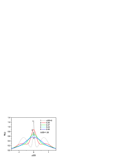
Figure 6: (Color online) Density of states of half–filled Anderson–Hubbard model for different degrees of disorder $\Delta$, and $U=2.5D$, typical for correlated metal.

In Fig. 6 we present our DMFT+$\Sigma$ results for the density of states, obtained for $U=2.5D=1.25W$ typical for correlated metal without disorder, for different degrees of disorder $\Delta$, including strong enough values, actually transforming correlated metal to correlated Anderson insulator (see next subsection IV.2). As may be expected, we observe typical widening and damping of DOS by disorder.

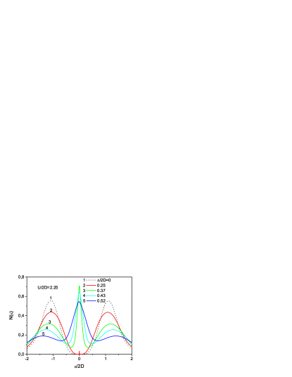
Figure 7: (Color online) Density of states of half–filled Anderson–Hubbard model for different degrees of disorder $\Delta$ and $U=4.5D$, typical for Mott insulator.

More unexpected are the results obtained for the values of $U$ typical for Mott insulator without disorder, as shown in Fig. 7 for $U=4.5D=2.25W$. We see the restoration of central peak (quasiparticle band) in DOS with the growth of disorder, transforming Mott insulator either to correlated metal or correlated Anderson insulator. Similar behavior of DOS was recently obtained in Ref. BV . However, in our calculations the presence of distinct Hubbard bands was observed even for rather large values of disorder, with no signs of vanishing Hubbard structure of DOS, which was observed in of Ref. BV . This is probably due to very simple nature of our approximation for DOS under disordering, though we must stress that this difference may be also due to another model of disorder used in Ref. BV , i.e. flat distribution of $\epsilon_{i}$ in (1) instead of our Gaussian case (2). Though unimportant, in general, to physics of Anderson transition, the type of disorder may be significant for the DOS behavior.

It is well known, that hysteresis behavior of DOS is obtained for Mott–Hubbard transition if we perform DMFT calculations with $U$ decreasing from insulating phase georges96 ; Bull . Mott insulator phase survives for the values of $U$ well inside the correlated metal phase, obtained with the increase of $U$. Metallic phase is restored at $U_{c1}\approx 1.0W$. The values of $U$ from the interval $U_{c1}<U<U_{c2}$ are usually considered as belonging to coexistence region of metallic and (Mott) insulating phases, with metallic phase being thermodynamically more stable georges96 ; Bull ; Blum .

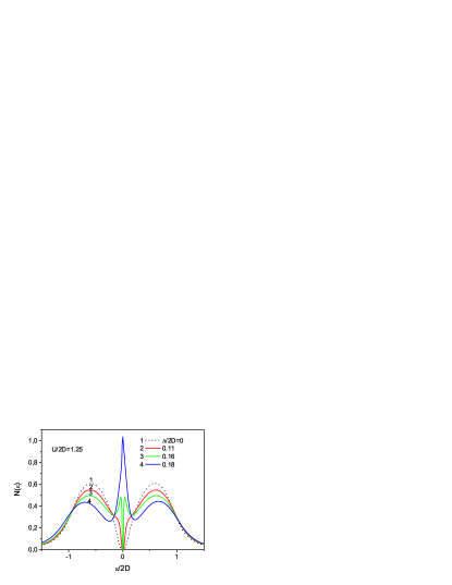
Figure 8: (Color online) Restoration of quasiparticle band by disorder in coexistence (hysteresis) region for $U=2.5D$, obtained from Mott insulator with decreasing $U$.

In Fig. 8 we present our typical data for DOS with different disorder for the same value of $U=2.5D=1.25W$ as in Fig. 6, but for hysteresis region, obtained by decreasing $U$ from Mott insulator phase. Again we observe the restoration of central peak (quasiparticle band) in DOS under disordering. Note also the peculiar form of DOS around the Fermi level during this transition – a narrow energy gap is conserved until it is closed by disorder, and central peak is formed from two symmetric maxima in DOS joining into quasiparticle band. This reminds similar behavior observed in periodic Anderson model georges96 . Apparently this effect was unnoticed in previous calculations of DOS in coexistence region Bull (in the absence of disorder), while in our case it was obtained mainly due to our use of very fine mesh of the values of disorder parameter $\Delta$.

The physical reason for rather unexpected restoration of the central (quasiparticle) peak in DOS is in fact clear. The controlling parameter for its appearance or disappearance in DMFT is actually the ratio of Hubbard interaction $U$ and the bare bandwidth $W=2D$. Under disordering we obtain the new effective bandwidth $W_{eff}$ (in the absence of Hubbard interaction) which grows with disorder, while semi–elliptic form of the DOS, with well–defined band edges is conserved in self–consistent Born approximation (9). This leads to the decrease of the ratio $U/W_{eff}$, which induces the reappearance of quasiparticle band in our model. This will be illustrated in more detail in subsection IV.3, where our DOS calculations within DMFT+$\Sigma$ approach for a wide range of parameters will be used to study the phase diagram of Anderson–Hubbard model.

IV.2 Dynamic conductivity: Mott–Hubbard and Anderson transitions

Real part of dynamic (optical) conductivity was calculated for different combinations of parameters of our model directly from Eqs. (37), (56) and (41) using the results of DMFT+$\Sigma$ loop (3) – (9) as an input. The values of conductivity below are given in natural units of ${e^{2}}/{\hbar a}$ ($a$ – lattice spacing).

In the absence of disorder we obviously reproduce the results of the standard DMFT pruschke ; georges96 with dynamic conductivity characterized in general by the usual (metallic) Drude–like peak at zero frequency and wide absorption maximum at $\omega\sim U$, corresponding to transitions to the upper Hubbard band. With the growth of $U$ Drude peak decreases and vanishes at Mott transition, when only transitions through the Mott–Hubbard gap contribute. Introduction of disorder leads to qualitative changes in the frequency dependence of conductivity. Below we mainly show the results obtained for the same values of $U$ and $\Delta$ as were used above to illustrate DOS behavior.

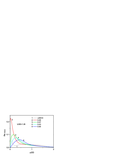
Figure 9: (Color online) Real part of dynamic conductivity for half–filled Anderson–Hubbard model for different degrees of disorder $\Delta$, and $U=2.5D$, typical for correlated metal. Lines 1,2 are for metallic phase, line 3 corresponds to the mobility edge (Anderson transition), lines 4,5 correspond to correlated Anderson insulator.

In Fig. 9 we present real part of dynamic (optical) conductivity for half–filled Anderson–Hubbard model for different degrees of disorder $\Delta$, and $U=2.5D$, typical for correlated metal. Transitions to upper Hubbard band at $\omega\sim U$ are practically unobservable in these data. However, it is clearly seen that metallic Drude peak at zero frequency is widened and suppressed, being gradually transformed to a peak at finite frequncies due to effects of Anderson localization. Anderson transition takes place at $\Delta_{c}\approx 0.74D=0.37W$ (which in all our graphs (including those for DOS) corresponds to curve 3). Note that this value is actually dependent on the value of cutoff (42), which is defined up to a constant of the order of unity MS86 ; Diagr . Naive expectations may have lead to a conclusion, that a narrow quasiparticle band at the Fermi level, which forms in general case of highly correlated metal, may be localized much more easily than typical conduction band. However, we see that these expectations are just wrong and this band is localized only at strong enough disorder $\Delta_{c}\sim D$, the same as for the whole conduction band of the width $\sim W$. This is in accordance with previous analysis of localization in two-band model ErkS .

More important is the fact that in DMFT+$\Sigma$ approximation the value of $\Delta_{c}$ is independent of $U$ as all interaction effects enter Eq. (41) only via $\Delta\Sigma^{RA}(\omega)\to 0$ for $\omega\to 0$ (at $T=0$), so that interaction just drops out at $\omega=0$. This is actually the main deficiency of our approximation, which is due to our neglect of interference effects between interaction and disorder scattering. Important role of these interference effects is known for a long time Lee85 ; ma . However, despite the neglect of these effects we are able to produce physically sound interpolation between two main limits of interest – pure Anderson transition due to disorder and Mott–Hubbard transition due to strong correlations. Thus we consider it as a reasonable first step to future complete theory of MIT in strongly correlated disordered systems.

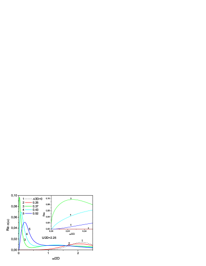
Figure 10: (Color online) Real part of dynamic conductivity of half–filled Anderson–Hubbard model for different degrees of disorder $\Delta$ and $U=4.5D$, typical for Mott insulator. Lines 1,2 correspond to Mott insulator, line 3 corresponds to the mobility edge (Anderson transition), lines 4,5 are for correlated Anderson insulator. Insert – enlarged region of small frequencies.

In Fig. 10 we present real part of dynamic (optical) conductivity for different degrees of disorder $\Delta$, and $U=4.5D$, typical for Mott–Hubbard insulator. At the insert we show our data for small frequencies, which allow clear distinction of different types of conductivity behavior, especially close to Anderson transition, or in Mott insulator phase. In this figure we clearly see the contribution of transitions to upper Hubbard band at $\omega\sim U$. More importantly we observe, that the growth of disorder produces finite conductivity within the frequency range of Mott–Hubbard gap, which correlates with the appearance of quasiparticle band (central peak) in DOS within this gap, as shown in Fig. 7. In general case, this conductivity is metallic (finite in the static limit of $\omega=0$) for $\Delta<\Delta_{c}$, while for $\Delta>\Delta_{c}$ at small frequencies we obtain ${\rm Re}\sigma(\omega)\sim\omega^{2}$, which is typical of Anderson insulator VW ; WV ; MS ; MS86 ; VW92 ; Diagr . Note that due to a finite internal accuracy of NRG numerics, small but finite spurious contributions to ${\rm Im}\Sigma^{R,A}(\varepsilon=0)$ always appear Bull and formally grow with $U$. These contributions are practically irrelevant in calculations of conductivity in metallic state. However, in Anderson insulator these spurious terms contribute via $\tilde{\omega}$ in Eq. (41) and lead to unphysical finite dephasing effects at $\omega=0$ (or $T=0$), which can simulate small finite static conductivity. To exclude these spurious effects we had to make appropriate subtractions in our data for ${\rm Im}\Sigma^{R,A}(\varepsilon)$ at $\varepsilon=0$.

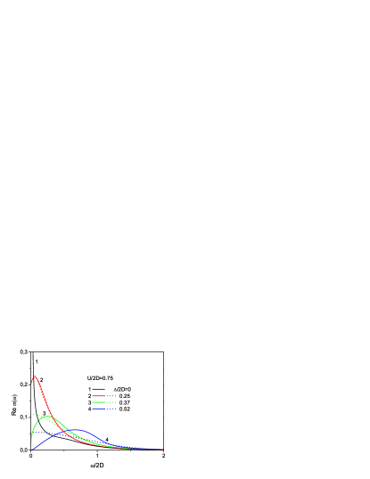
Figure 11: (Color online) Real part of dynamic conductivity of half–filled Anderson–Hubbard model for different degrees of disorder $\Delta$ and $U=1.5D$, comparison of self–consistent theory (full lines) with “ladder” approximation (dotted lines).

Rather unusual is the appearance of low frequency peak in ${\rm Re}\sigma(\omega)$ at low frequencies even in metallic phase. This is due to importance of weak localization effects, as can be clearly seen from Fig. 11, where we compare the real part of dynamic conductivity for different degrees of disorder $\Delta$ and $U=1.5D$, obtained via our self–consistent approach (taking into account localization effects via “maximally crossed” diagrams) with that obtained using the “ladder” approximation for $\Phi^{0RA}_{\varepsilon}(\omega,{\bf q})$ (similar to (56)), which neglects all localization effects. It is clearly seen that in this simple approximation we just obtain the usual Drude–like peak at $\omega=0$, while the account of localization effects produce the peak in ${\rm Re}\sigma(\omega)$ at low (finite) frequencies. Metallic state is defined Mott90 by the finite value of zero temperature conductivity at $\omega=0$.

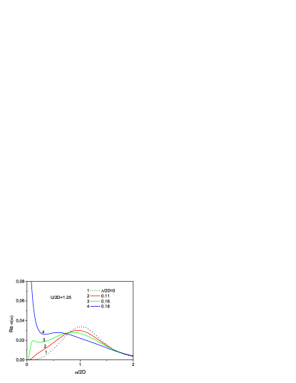
Figure 12: (Color online) Real part of dynamic conductivity of half–filled Anderson–Hubbard model for different degrees of disorder $\Delta$ and $U=2.5D$, obtained from Mott insulator with decreasing $U$.

Up to now we presented only conductivity data obtained with increase of $U$ from metallic to (Mott) insulating phase. As we decrease $U$ from Mott insulator hysteresis of conductivity is observed in coexistence region, defined (in the absence of disorder, $\Delta=0$) by $U_{c1}<U<U_{c2}$. Typical data are shown in Fig. 12, where we present the real part of dynamic conductivity for different degrees of disorder $\Delta$ and $U=2.5D$, obtained from Mott insulator with decreasing $U$, which should be compared with those shown in Fig. 9. Transition to metallic state via the closure of a narrow gap, “inside” much wider Mott–Hubbard gap, is clearly seen, which correlates with DOS data shown in Fig. 8.

IV.3 Phase diagram of half–filled Anderson–Hubbard model.

Phase diagram of half–filled Anderson–Hubbard model was studied in Ref. BV , using the approach, based on direct DMFT calculations for a set of random realizations of site energies $\epsilon_{i}$ in (1) with subsequent averaging to get both the standard average DOS and also geometrically averaged local DOS, which was used to determine transition to Anderson insulator phase. Here we present our results for the zero–temperature phase diagram of half–filled paramagnetic Anderson–Hubbard model, obtained from extensive calculations of both average DOS and dynamic (optical) conductivity in DMFT+$\Sigma$ approximation. It should be noted, that conductivity calculations are the most direct way to distinguish metallic and insulating phases Mott90 .

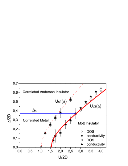
Figure 13: (Color online) Zero temperature phase diagram of paramagnetic Anderson–Hubbard model. Borders of Mott insulator phase $U_{c1,c2}(\Delta)$ are shown as obtained from Eqs. (46), while different symbols show values calculated either from DOS or conductivity behavior. Dotted line defines the border of coexistence region obtained with decreasing $U$ from Mott insulator phase. Line of Anderson transition is given by calculated value of $\Delta_{c}=0.37$.

Our phase diagram in the disorder–correlation $(\Delta,U)$–plane is shown in Fig. 13. Anderson transition line $\Delta_{c}\approx 0.37W=0.74D$ was determined as the value of disorder for which the static conductivity becomes zero at $T=0$. Mott–Hubbard transition may be determined either via the disappearance of central peak (quasiparticle band) in DOS, or from conductivity, e.g. looking for the closure of gap in dynamic conductivity in insulating phase, or from vanishing static conductivity in metallic region. All these methods were used and appropriate results are shown for comparison in Fig. 13.

We already stressed that DMFT+$\Sigma$ approximation gives the universal ($U$–independent) value of $\Delta_{c}$. This is due to neglect of interference between disorder scattering and Hubbard interaction, and leads to the main (over) simplification of our phase diagram, compared with that obtained in Ref.BV . Note, that direct comparison of our critical disorder value with those of Ref. BV is complicated by different types of random site–energies distributions used here (Gaussian) and in Ref. BV (rectangular distribution). As a rule of thumb (cf. second reference in MS ) our Gaussian value of $\Delta_{c}$ should be multiplied by $\sqrt{12}$ to obtain the critical disorder value for rectangular distribution. This gives $\Delta_{c}\approx 1.28$ in rather good agreement with $\Delta_{c}(U=0)\approx 1.35W$ value of Ref. BV , justifying our cutoff choice in (42).

The influence of disorder scattering on Mott–Hubbard transition is highly non–trivial and in some respects is in qualitative agreement with results of Ref. BV . The main difference is that our data indicate the survival of Hubbard bands structures in DOS even in the limit of rather large disorder, while these were claimed to disappear in Ref. BV . Also we obtain the coexistence region smoothly widening with the growth of disorder and not disappearing at some “critical” point, as in Ref. BV . The borders of our coexistence region, which in fact define the borders of Mott insulator phase obtained with increasing or decreasing $U$, are determined by the lines of $U_{c1}(\Delta)$ and $U_{c2}(\Delta)$ shown in Fig. 13, which are obtained from the simple equation:

$$\frac{U_{c1,c2}(\Delta)}{W_{eff}}=\frac{U_{c1,c2}}{W}$$ (44)

with

$$W_{eff}=W\sqrt{1+16\frac{\Delta^{2}}{W^{2}}}$$ (45)

which is the effective bandwidth in the presence of disorder, calculated for $U=0$ in self–consistent Born approximation (9). Thus the borders of coexistence region are given by:

$$U_{c1,c2}(\Delta)=U_{c1,c2}\sqrt{1+16\frac{\Delta^{2}}{W^{2}}}$$ (46)

which are explicitly shown in Fig. 13 by dotted and full lines, defining the borders of Mott insulator phase. Numerical results for disappearance of quasiparticle band (central peak) in DOS, as well as points following from qualitative change in conductivity behavior, are shown in Fig. 13 by different symbols demonstrating very good agreement with these lines, confirming the ratio (44) as controlling parameter of Mott transition in the presence of disorder.

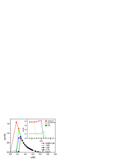
Figure 14: (Color online) Disorder dependence of static conductivity, obtained for several values of $U$ and showing disorder induced Mott insulator to metal transition. At the insert we show static conductivity dependence on $U$ close to Mott transition, including typical hysteresis behavior obtained with $U$ decreasing from Mott insulator phase.

Most striking result of our analysis (also qualitatively demonstrated in Ref. BV ) is the possibility of metallic state being restored from Mott–Hubbard insulator with the growth of disorder. This is clear from the phase diagram and is nicely demonstrated by our data for (static) conductivity shown in Fig. 14 for several values of $U>U_{c2}$ and disorder values $\Delta<\Delta_{c}$. At the insert in Fig. 14 we also illustrate static conductivity hysteresis, observed in coexistence region of the phase diagram, obtained with $U$ decreasing from Mott insulator phase.

IV.4 Doped Mott insulator

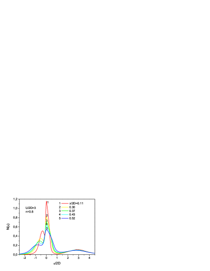
Figure 15: (Color online) Density of states of Anderson–Hubbard model with electron concentration $n=0.8$ for different degrees of disorder $\Delta$ and $U=6.0D$, representing the doped Mott insulator.

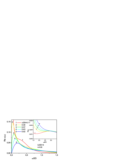
Figure 16: (Color online) Real part of dynamic conductivity of Anderson–Hubbard model with electron concentration $n=0.8$ for different degrees of disorder $\Delta$ and $U=6.0D$, representing the doped Mott insulator. Insert – high frequency behavior with signs of transitions to the upper Hubbard band.

All results presented above were obtained for half–filled case. Here we briefly consider deviations from half–filling. In metallic phase, doping from half–filling does not produce any qualitative changes in conductivity behavior, which only demonstrates Anderson transition with the growth of disorder. Thus we shall concentrate only on the case of doped Mott insulator. Strictly speaking, for non half–filled case we never obtain Mott–Hubbard insulator in DMFT at all. In Fig. 15 we show the density of states of Anderson–Hubbard model with electron concentration $n=0.8$ for different degrees of disorder $\Delta$ and $U=6.0D$, representing typical case of the doped Mott insulator. Quasiparticle band overlaps now with lower Hubbard band and is smeared by disorder, which is just the expected behavior in metallic state. Nothing spectacular happens also with conductivity, which is shown for the same set of parameters in Fig. 16. It shows typical behavior associated with disorder induced Anderson MIT. Small signs of transitions to the upper Hubbard band can be seen for $\omega\sim U$ (see insert in Fig. 16). Thus, doped Mott insulator with disorder is qualitatively quite similar to the case of disordered correlated metal discussed above.

V Conclusion

We used a generalized DMFT+$\Sigma$ approach to calculate basic properties of disordered Hubbard model. The main advantage of our method is its ability to provide rather simple interpolation scheme between rather well understood cases of strongly correlated system (DMFT and Mott–Hubbard MIT) and that of strongly disordered metal without Hubbard correlations, undergoing Anderson MIT. Apparently this interpolation scheme captures the main qualitative features of Anderson–Hubbard model, such as the general behavior of DOS and dynamic (optical) conductivity. The overall picture of zero–temperature phase diagram is also quite reasonable and is satisfactory agreement with the results of more elaborate numerical work BV . Actually, our DMFT+$\Sigma$ approach is much less time–consuming than more direct numerical approaches, such as that of Ref. BV , and in fact allows us to calculate all basic (measurable) physical characteristics of Anderson–Hubbard model.

Main shortcoming of our approach is its neglect of interference effects of disorder scattering and Hubbard interaction, which leads to independence of Anderson MIT critical disorder $\Delta_{c}$ on interaction $U$. Importance of interference effects is known for a long time Lee85 ; ma , but its account was only partially successful in case of weak correlations. At the same time, the neglect of these interference effects is the major approximation of DMFT+$\Sigma$, allowing to derive rather simple and physical interpolation scheme, allowing the analysis of the limit of strong correlations. Attempts to include interference effects in our scheme are postponed for future work.

Another simplification is, of course, our assumption of non–magnetic (paramagnetic) ground state of Anderson–Hubbard model. The importance of magnetic (spin) effects in strongly correlated systems is well known, as well as the problem of competition of ground states with different types of magnetic ordering georges96 . Importance of disorder in the studies of interplay of these possible ground states is also quite evident. These may also be the subject of our future work.

Despite these shortcomings, our results seem very promising, especially concerning the influence of strong disorder on Mott–Hubbard MIT and the overall form of the phase diagram at zero temperature. The changes in phase diagram at finite temperatures will be the subject of further studies. Non–trivial predictions of our approach, such as the general behavior of dynamic (optical) conductivity and, especially, the prediction of disorder induced Mott insulator to metal transition can be the subject of direct experimental verification.

VI Acknowledgements

We are grateful to Th. Pruschke for providing us with his effective NRG code. This work was supported in part by RFBR grants 05-02-16301 (MS,EK,IN), 05-02-17244 (IN), 06-02-90537 (IN), by the joint UrO-SO project (EK,IN), and programs of the Presidium of the Russian Academy of Sciences (RAS) “Quantum macrophysics” and of the Division of Physical Sciences of the RAS “Strongly correlated electrons in semiconductors, metals, superconductors and magnetic materials”. I.N. acknowledges support from the Dynasty Foundation, International Center for Fundamental Physics in Moscow program for young scientists and from grant of the President of Russian Federation for young PhD MK-2118.2005.02.

Appendix A Equation for relaxation kernel

Let us follow the standard approach of self–consistent theory of localization VW ; WV ; MS ; MS86 ; VW92 ; Diagr , taking into account the DMFT contributions $\Sigma^{R,A}(\varepsilon)$ in single-particle Green’s functions (30) and not limiting ourselves to the usual limit of small $\omega$.

Consider Bethe–Salpeter equation relating the full two-particle Green’s function $\Phi^{0RA}_{\bf pp^{\prime}}(\omega,{\bf q})$ to irreducible vertex $U^{0RA}_{\bf pp^{\prime}}(\omega,{\bf q})$, accounting only for impurity scattering in vertices, but built upon Green’s functions given by (30). This equation can be written now as a generalized kinetic equation of the following form VW ; WV ; MS ; MS86 ; VW92 ; Diagr :

$$\left(\tilde{\omega}-\epsilon({\bf p})-\Delta\Sigma^{RA}_{imp}(\omega)\right)\Phi^{0RA}_{\bf pp^{\prime}}(\omega,{\bf q})=$$

$$=-\Delta G_{\bf p}\left(\delta_{\bf pp^{\prime}}+\sum_{\bf p_{1}}U^{0RA}_{\bf pp_{1}}(\omega,{\bf q})\Phi^{0RA}_{\bf p_{1}p^{\prime}}(\omega,{\bf q})\right)$$ (47)

where $\Delta G_{\bf p}=G^{R}(\varepsilon_{+},{\bf p}_{+})-G^{A}(\varepsilon_{-},{\bf p}_{-})$. The main difference with similar equation of Refs. VW ; WV ; MS ; MS86 ; VW92 ; Diagr is the replacement $\omega\to\tilde{\omega}$.

Let us sum both sides of (47) and of the same equation multiplied by $({\bf{\hat{p}}{\hat{q}}})$ (where ${\bf{\hat{p}}}=\frac{\bf p}{|{\bf p}|}$ and ${\bf{\hat{q}}}=\frac{\bf q}{|{\bf q}|}$ are appropriate unit vectors) over ${\bf p}$ and ${\bf p^{\prime}}$, taking into account an exact Ward identity VW :

$$\Delta\Sigma^{RA}_{imp}(\omega)=\sum_{\bf p^{\prime}}U^{0RA}_{\bf pp^{\prime}}(\omega,{\bf q})\Delta G_{\bf p^{\prime}}$$ (48)

and using an approximate representation (cf. Ref.VW )

$$\sum_{\bf p^{\prime}}\Phi^{0RA}_{\bf pp^{\prime}}(\omega,{\bf q})\approx\frac{\Delta G_{\bf p}}{\sum_{\bf p}\Delta G_{\bf p}}\Phi^{0RA}_{\varepsilon}(\omega,{\bf q})+$$

$$+\frac{\Delta G_{\bf p}({\bf{\hat{p}}{\hat{q}}})}{\sum_{\bf p}\Delta G_{\bf p}({\bf{\hat{p}}{\hat{q}}})^{2}}\Phi^{0RA}_{1\varepsilon}(\omega,{\bf q})$$ (49)

where $\Phi^{0RA}_{\varepsilon}(\omega,{\bf q})=\sum_{\bf pp^{\prime}}\Phi^{0RA}_{\bf pp^{\prime}}(\omega,{\bf q})$ is our loop (28), while $\Phi^{0RA}_{1\varepsilon}(\omega,{\bf q})=\sum_{\bf pp^{\prime}}({\bf{\hat{p}}{\hat{q}}})\Phi^{0RA}_{\bf pp^{\prime}}(\omega,{\bf q})$. Important difference from similar representation used in Refs. VW ; WV ; MS ; MS86 ; VW92 ; Diagr is that (49) is not limited to small $\omega$.

Now (for $q\to 0$) we obtain the following closed system of equations defining both $\Phi^{0RA}_{\varepsilon}(\omega,{\bf q})$ and $\Phi^{0RA}_{1\varepsilon}(\omega,{\bf q})$:

$$\tilde{\omega}\Phi^{0RA}_{\varepsilon}(\omega,{\bf q})-<v>q\Phi^{0RA}_{1\varepsilon}(\omega,{\bf q})=-\sum_{\bf p}\Delta G_{\bf p}$$ (50)

$$(\tilde{\omega}+M(\omega))\Phi^{0RA}_{1\varepsilon}(\omega,{\bf q})-\frac{<v>}{d}q\Phi^{0RA}_{1\varepsilon}(\omega,{\bf q})=0\\$$

where relaxation kernel is given by:

$$M(\omega)=-\Delta\Sigma^{RA}_{imp}(\omega)+$$

$$+d\frac{\sum_{\bf pp^{\prime}}({\bf{\hat{p}}{\hat{q}}})\Delta G_{\bf p}U^{0RA}_{\bf pp^{\prime}}(\omega,{\bf q})\Delta G_{\bf p^{\prime}}({\bf{\hat{p}^{\prime}}{\hat{q}}})}{\sum_{\bf p}\Delta G_{\bf p}},$$ (51)

with average velocity $<v>$ defined as:

$$<v>=\frac{\sum_{\bf p}|{\bf v}_{\bf p}|\Delta G_{\bf p}}{\sum_{\bf p}\Delta G_{\bf p}};\\ \ {\bf v}_{\bf p}=\frac{\partial\epsilon({\bf p})}{\partial{\bf p}},$$ (52)

From (50) we immediately obtain:

$$\Phi^{0RA}_{\varepsilon}({\bf q},\tilde{\omega})=\frac{-\sum_{\bf p}\Delta G_{\bf p}}{\tilde{\omega}+iD(\omega)q^{2}}$$ (53)

which for small $\omega$ reduces to (33) with generalized diffusion coefficient given by (38).

Using for irreducible vertex $U^{0RA}_{\bf pp^{\prime}}(\omega,{\bf q})$ an approximation of “maximally crossed” diagrams and introducing the standard self-consistency procedure of Refs.VW ; WV ; MS ; MS86 ; VW92 ; Diagr (i.e. replacing the Drude diffusion coefficient in Cooperon contribution to irreducible vertex by the generalized one defined by (38)), we obtain from (51) our expression (39) for relaxation kernel.

Our equation (41) for the generalized diffusion coefficient (which is in general case complex) reduces just to the usual transcendent equation. It was solved by iterations for every value of $\tilde{\omega}$, taking into account that for $d=3$ and cutoff given by (42), the sum entering (41) reduces to:

$$\sum_{\bf q}\frac{1}{\tilde{\omega}+iD(\omega)q^{2}}=\frac{1}{2\pi^{2}}\frac{k_{0}^{3}}{iD(\omega)k_{0}^{2}}\int_{0}^{1}\frac{y^{2}dy}{y^{2}+\frac{\tilde{\omega}}{iD(\omega)k_{0}^{2}}}=$$ (54)

$$=\frac{1}{2\pi^{2}}\frac{k_{0}^{3}}{iD(\omega)k_{0}^{2}}\left\{1-{\left(\frac{\tilde{\omega}}{iD(\omega)k_{0}^{2}}\right)}^{\frac{1}{2}}arctg\left({\left(\frac{iD(\omega)k_{0}^{2}}{\tilde{\omega}}\right)}^{\frac{1}{2}}\right)\right\}\\$$

For finite frequencies $\omega$ we use $\Phi^{0RA}_{\varepsilon}({\bf q},\tilde{\omega})$ given by (53), so that an expression (25) for dynamic conductivity is to be rewritten as:

$${\rm{Re}}\sigma(\omega)=\frac{e^{2}\omega}{2\pi}\int_{-\infty}^{\infty}d\varepsilon\left[f(\varepsilon_{-})-f(\varepsilon_{+})\right]\times$$

$${\rm Re}\left\{\frac{i\sum_{\bf p}\Delta G_{\bf p}D(\omega)}{\omega^{2}}-\phi^{0RR}_{\varepsilon}(\omega)\left[1-\frac{\Delta\Sigma^{RR}(\omega)}{\omega}\right]^{2}\right\},$$

(55)

The second term here was taken in the “ladder” approximation:

$$\Phi^{0RR}_{\varepsilon}(\omega,{\bf q})=\frac{\sum_{\bf p}G^{R}(\varepsilon_{+},{\bf p}_{+})G^{R}(\varepsilon_{-},{\bf p}_{-})}{1-\Delta^{2}\sum_{\bf p}G^{R}(\varepsilon_{+},{\bf p}_{+})G^{R}(\varepsilon_{-},{\bf p}_{-})}$$ (56)

This contribution (non singular at small $\omega$) is irrelevant for conductivity at small $\omega\to 0$, but leads to finite corrections with increasing $\omega$. Eq. (55) is our final result, which was analyzed numerically in a wide interval of frequencies (for small $\omega$ it reduces to (37)).

Appendix B “Bare” electron dispersion and velocity

We consider the “bare” energy band with semi-elliptic DOS (43). Assuming isotropic electron spectrum $\epsilon({\bf p})=\epsilon(|{\bf p}|)\equiv\epsilon(p)$ and equating the number of states in spherical layer of momentum space to the number of states in an energy interval $[\epsilon,\epsilon+d\epsilon]$], we obtain differential equation determining the energy dispersion $\epsilon(p)$:

$$\frac{4\pi p^{2}dp}{(2\pi)^{3}}=N_{0}(\epsilon)d\epsilon$$ (57)

For quadratic energy dispersion $\epsilon(p)$ close to the lower band edge we get the initial condition for Eq. (57) for $p\to 0$ and $\epsilon\to-D$. Then we obtain

$$p={\left[6\pi\left(\pi-\varphi+\frac{1}{2}sin(2\varphi)\right)\right]}^{\frac{1}{3}}$$ (58)

with $\varphi=arccos(\frac{\epsilon}{D})$ and momentum in units of inverse lattice spacing. Eq. (58) implicitly defines “bare” energy dispersion $\epsilon(p)$ for electronic part of the spectrum $\epsilon\in[-D,0]$.

For half-filled band we easily determine the Fermi momentum as:

$$p_{F}=p(\epsilon=0)={\left(3\pi^{2}\right)}^{\frac{1}{3}}$$ (59)

We also need electron velocity $|{\bf v_{p}}|=\left|\frac{\partial\epsilon({\bf p})}{\partial{\bf p}}\right|=\frac{\partial\epsilon(p)}{\partial p}$ entering into the expression (52) for average velocity. From (57) we obtain:

$$|{\bf v_{p}}|=\frac{d\epsilon}{dp}=\frac{p^{2}}{2\pi^{2}}\frac{1}{N_{0}(\epsilon)}$$ (60)

where $p$ is given by Eq. (58).

To obtain quadratic dispersion for hole part of the spectrum ($\epsilon\in[0,D]$) close to the upper band edge ($\epsilon\to D$) we introduce the hole momentum $\tilde{p}=2p_{F}-p$ and write similarly to (57):

$$\frac{4\pi\tilde{p}^{2}d\tilde{p}}{(2\pi)^{3}}=-N_{0}(\epsilon)d\epsilon$$ (61)

Putting $\tilde{p}\to 0$ at the upper band edge $\epsilon\to 0$, we get:

$$\tilde{p}={\left[6\pi\left(\varphi-\frac{1}{2}sin(2\varphi)\right)\right]}^{\frac{1}{3}}$$ (62)

Then for velocity at the hole part of the spectrum we obtain:

$$|{\bf v_{p}}|=\frac{d\epsilon}{dp}=-\frac{d\epsilon}{d\tilde{p}}=\frac{\tilde{p}^{2}}{2\pi^{2}}\frac{1}{N_{0}(\epsilon)}$$ (63)

Eqs. (60) and (63) define energy dependence of $|{\bf v_{p}}|$. It is easily seen that velocity is even in energy and becomes zero at the band edges. These expressions allow us to change from momentum summation (e.g. in Eq. (52)) to energy integration.

References

- (1)
- (2) P. A. Lee and T. V. Ramakrishnan, Rev. Mod. Phys. 57, 287 (1985); D. Belitz and T. R. Kirkpatrick, Rev. Mod. Phys. 66, 261 (1994).
- (3) N. F. Mott, Proc. Phys. Soc. A 62, 416 (1949); Metal–Insulator Transitions, 2nd edn. (Taylor and Francis, London 1990).
- (4) P. W. Anderson, Phys. Rev. 109, 1492 (1958).
- (5) A. M. Finkelshtein, Sov. Phys. JEPT 75, 97 (1983); C. Castellani et al., Phys. Rev. B 30, 527 (1984).
- (6) W. Metzner and D. Vollhardt, Phys. Rev. Lett. 62, 324 (1989).
- (7) D. Vollhardt, in Correlated Electron Systems, edited by V. J. Emery, World Scientific, Singapore, 1993, p. 57.
- (8) Th. Pruschke, M. Jarrell, and J. K. Freericks, Adv. Phys. 44, 187 (1995).
- (9) A. Georges, G. Kotliar, W. Krauth, and M. J. Rozenberg, Rev. Mod. Phys. 68, 13 (1996).
- (10) M. Ulmke, V. Janiš, and D. Vollhardt, Phys. Rev. B 51, 10411 (1995).
- (11) R. Vlaming and D. Vollhardt, Phys. Rev. B 45, 4637 (1992).
- (12) V. Dobrosavljević and G. Kotliar, Phys. Rev. Lett. 78, 3943 (1997).
- (13) V. Dobrosavljević, A. A. Pastor, and B. K. Nikolić, Europhys. Lett. 62, 76 (2003).
- (14) K. Byczuk, W. Hofstetter, D. Vollhardt. Phys. Rev. Lett. 94, 056404 (2005)
- (15) D. Vollhardt and P. Wölfle, Phys. Rev. B 22, 4666 (1980); Phys. Rev. Lett. 48, 699 (1982)
- (16) P. Wölfle and D. Vollhardt, in Anderson Localization, eds. Y. Nagaoka and H. Fukuyama, Springer Series in Solis State Sciences, vol. 39, p.26. Springer Verlag, Berlin 1982.
- (17) A.V. Myasnikov, M.V. Sadovskii, Fiz. Tverd. Tela 24, 3569 (1982) [Sov. Phys.-Solid State 24, 2033 (1982) ]; E.A. Kotov, M.V. Sadovskii. Zs. Phys. B 51, 17 (1983).
- (18) M.V. Sadovskii, in Soviet Scientific Reviews – Physics Reviews, ed. I.M. Khalatnikov, vol. 7, p.1. Harwood Academic Publ., NY 1986.
- (19) D. Vollhardt, P. Wölfle, in Electronic Phase Transitions, eds. W. Hanke and Yu.V. Kopaev, vol. 32, p. 1. North–Holland, Amsterdam 1992.
- (20) M.V. Sadovskii. Diagrammatics. World Scientific, Singapore 2006.
- (21) E.Z. Kuchinskii, M.V. Sadovskii, V.G. Suvorov. Zh. Eksp. Teor. Fiz. 107, 2027 (1995) [JETP 80, 1122 (1995)]; E.Z. Kuhinskii, M.A. Erkabaev. Fiz. Tverd. Tela 39, 412 (1997).
- (22) E.Z.Kuchinskii, I.A.Nekrasov, M.V.Sadovskii. Pis’ma Zh. Eksp. Teor. Fiz. 82, 217 (2005) [JETP Lett. 82, 198 (2005)].
- (23) M.V. Sadovskii, I.A. Nekrasov, E.Z. Kuchinskii, Th. Prushke, V.I. Anisimov. Phys. Rev. B 72, 155105 (2005).
- (24) E.Z. Kuchinskii, I.A. Nekrasov, M.V. Sadovskii. Fizika Nizkikh Temperatur 32, 528 (2006) [Low Temp. Phys. 32, 398 (2006)].
- (25) E.Z. Kuchinskii, I.A. Nekrasov, M.V. Sadovskii. Phys. Rev. B 75, 115102 (2007).
- (26) K.G. Wilson, Rev. Mod. Phys. 47, 773 (1975); H.R. Krishna-murthy, J.W. Wilkins, and K.G. Wilson, Phys. Rev. B 21, 1003 (1980); ibid. 21, 1044 (1980); A.C. Hewson, The Kondo Problem to Heavy Fermions. Cambridge University Press, 1993.
- (27) R. Bulla, A.C. Hewson and Th. Pruschke, J. Phys. – Condens. Matter 10, 8365(1998).
- (28) R. Bulla, Phys. Rev. Lett. 83, 136 (1999); R. Bulla, T.A. Costi and D. Vollhardt. Phys. Rev. B 64, 045103 (2001).
- (29) A.B. Migdal. Theory of Finite Fermi Systems and Applications to Atomic Nuclei. Interscience Publishers, NY 1967.
- (30) N. Blümer. Mott–Hubbard Metal–Insulator Transition and Optical Conductivity, Thesis, München 2002.
- (31) M.A. Erkabaev, M.V. Sadovskii. J. Moscow Phys. Soc. 2, 233 (1992)