Transverse Emittance Dilution due to Coupler Kicks in Linear Accelerators

Abstract

One of the main concerns in the design of low emittance linear accelerators (linacs) is the preservation of beam emittance. Here we discuss one possible source of emittance dilution, the coupler kick, due to transverse electromagnetic fields in the accelerating cavities of the linac caused by the power coupler geometry. In addition to emittance growth, the coupler kick also produces orbit distortions. It is common wisdom that emittance growth from coupler kicks can be strongly reduced by using two couplers per cavity mounted opposite each other or by having the couplers of successive cavities alternation from above to below the beam pipe so as to cancel each individual kick. While this is correct, including two couplers per cavity or alternating the coupler location requires large technical changes and increased cost for superconducting cryomodules where cryogenic pipes are arranged parallel to a string of several cavities. We therefore analyze consequences of alternate coupler placements.

We show here that alternating the coupler location from above to below compensates the emittance growth as well as the orbit distortions. And for sufficiently large Q values, alternating the coupler location from before to after the cavity leads to a cancellation of the orbit distortion but not of the emittance growth, whereas alternating the coupler location from before and above to behind and below the cavity cancels the emittance growth but not the orbit distortion. We show that cancellations hold for sufficiently large Q values. These compensations hold even when each cavity is individually detuned, e.g. by microphonics. Another effective method for reducing coupler kicks that is studied is the optimization of the phase of the coupler kick so as to minimize the effects on emittance from each coupler. This technique is independent of the coupler geometry but relies on operating on crest. A final technique studied is symmetrization of the cavity geometry in the coupler region with the addition of a stub opposite the coupler. This technique works by reducing the amplitude of the off axis fields and is thus effective for off crest acceleration as well.

We show applications of these techniques to the energy recovery linac (ERL) planned at Cornell University.

I Introduction

A possible source of emittance dilution in an accelerating cavity is that caused by the input power coupler. The addition of a single coupler situated perpendicular to the beam pipe creates an asymmetry in the cavity geometry, leading to non radially symmetric field profiles in the beam pipe in the vicinity of the coupler Zhang . The asymmetric fields produce a transverse radio frequency (rf) kick to an accelerating bunch resulting in an increase in emittance Dohlus . Additionally, the coupler region will change the cavities’ RF focusing somewhat because the transverse dependence of fields in this region is different to that in the main cavity. This effect changes the emittance growth due to cavity focusing, but it is not considered part of the coupler kick and is not discussed here. Previous studies have found the effect on emittance due to the transverse rf kick to be significant in the injector cavities of the Cornell energy recovery linac (ERL) Belomestnykh02 ; shemelin ; Greenwald . As a solution, a second input coupler was installed situated on the opposite side of the beam pipe, canceling the asymmetry and the transverse kick shemelin3 . This approach, though effective, would be both a technically challenging and expensive design for a large superconducting linac such as the Cornell ERL or the ILC. A solution to the emittance increase due to coupler kicks that does not include the addition of a second coupler would therefore be preferable.

In this paper we investigate the effects from a transverse rf-coupler kick on the emittance of a Gaussian bunch and discuss possible methods of reducing emittance growth. We consider and compare the effects from six different coupler configurations: (tf) all couplers mounted on the top of the beam pipe; all couplers placed in front of the cavity, (ta) all couplers mounted on the top of the beam pipe; couplers alternated from being placed in front of and behind the cavity each cavity, (af) couplers alternated from being mounted on top of and underneath the beam pipe each cavity; all couplers placed in front of the cavity, (aa) couplers alternated from being mounted on top of and underneath the beam pipe each cavity; couplers alternated from being placed in front of and behind the cavity each cavity, (mf) couplers alternated from being mounted on top of and underneath the beam pipe each cryomodule, or every ten cavities; all couplers placed in front of the cavity, (dc) double coupler arrangement with two couplers per cavity, equivalent to no transverse kick. The proposed design for the Cornell ERL includes alternating the coupler placement from in front of and behind the cavity each cavity, as in configurations (ta) and (aa). The configurations (tf) and (af) are included for comparison so as to investigate the effects from alternating the placement of the coupler from front to back. The (mf) configuration is included so as to investigate the extent of the cancellation between two cryomodules. Of the two configurations (ta) and (aa) the most preferable would be configuration (ta) as it includes mounting couplers all on the same side of the beam pipe and is thus technically more feasible. In addition to these six configurations we investigate the effects due to optimizing the placement of the coupler along the beam pipe and the effects due to the addition of a symmetrizing stub opposite the coupler.

Table 1: Parameters of accelerating cavities for the Cornell ERL.

Frequency	1300 MHz
Number of Cells	7
Cavity Shape	TESLA type
Accelerating Voltage	15 MV/m
$Q_{0}$	$10^{10}$
$Q_{ext}$	$10^{8}$
Coupler Type	Coaxial
Coax Impedance	50 $\Omega$

We simulate, using Microwave Studios (MWS) MWS , the electric and magnetic standing wave profiles inside an accelerating cavity with the coaxial coupler included (Fig. 1). The cavity used for simulation is a two cell model of the seven cell TESLA-type cavity to be used in the proposed Cornell ERL. A two cell cavity instead of a seven cell cavity is used in order to limit the simulation time. From the standing wave profiles of MWS, complex traveling waves are modeled of which the real parts represent the true waves in the cavity. A numerical integration of these waves is performed along the central cavity axis to calculate the total change in momentum of a charged particle traveling through the cavity. The coupler kick, defined as the ratio of the transverse change in momentum and the change in momentum along the cavity axis, is calculated and input into a lattice representing the proposed Cornell ERL. A simulation of an electron bunch through the lattice is done with BMAD sagan and the total normalized emittance growth is calculated and compared for all mentioned configurations.

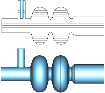
Figure 1: Two cell model of the seven cell TESLA type Cornell ERL superconducting rf cavity.

We find that due to the high $Q_{ext}$ values of the accelerating cavities, the fields on the cavity axis, including those in the vicinity of the coupler, are very well approximated by standing waves. From this approximation we formulate analytical arguments to support the results from our simulation, namely that the orbit distortion is canceled. Furthermore, from the standing wave approximation, we present arguments to back up the results from simulations indicating that the coupler kick is independent of reflected waves in the coupler and of relative phase differences between incoming and reflected waves. Thus our result of the cancellation of the coupler kick between adjacent cavities is unaffected by cavity detuning.

Lastly, we show that placing the coupler at a distance from the entrance of the cavity so as to match the phases of the coupler kick and accelerating kick minimizes the emittance increase, as does the addition of a symmetrizing stub which effectively minimizes the amplitudes of the off axis fields in the beam pipe. This additionally minimizes the orbit distortion. Important to note is that emittance growth due to higher order mode (HOM) couplers can be dealt with using all of the above techniques in an analogous way.

The Linac parameters used for simulations of the Cornell ERL are listed in Table 1.

II Emittance Growth due to Coupler Kick

In this section an analytical expression is derived for the change in emittance of a relativistic, Gaussian distributed bunch due to a transverse rf kick in an accelerating rf cavity. We begin by defining the change in transverse momentum, in this case the y component:

$$\Delta P_{y}=\frac{\Delta E_{0}}{c}|\kappa|e^{i[\phi_{c}+\psi+\omega(t-t_{0})]}\ ,\ \ \Delta p_{y}=Re\{\Delta P_{y}\}.$$ (1)

In the above, $Re\{(\Delta E_{0}/c)e^{i[\psi+\omega(t-t_{0})]}\}$ is the change in momentum in the longitudinal direction, $p_{s}=Re\{\Delta P_{s}\}$, for a particle at an offset $\Delta t=t-t_{0}$ from the center of the bunch. The coupler kick $\kappa$ is defined as the ratio of the complex transverse rf kick with the complex longitudinal kick Dohlus2 :

$$\kappa=\frac{\Delta P_{y}}{\Delta P_{s}}$$ (2)

The phase of the coupler kick, $\phi_{c}$, is the difference between the phase of the the transverse kick and $\psi$, the phase of the accelerating kick with respect to the reference particle at the center of the bunch. Dividing by the initial longitudinal momentum $E/c$ we achieve the change in the phase space component $y^{\prime}$:

$$\Delta y^{\prime}=Re\{\frac{\Delta E_{0}}{E}|\kappa|e^{i(\phi_{c}+\psi+\omega\Delta t)}\}.$$ (3)

Expanding to first order in $\Delta t$ leads to the approximate expression

$$\Delta y^{\prime} \approx Re\{\frac{\Delta E_{0}}{E}|\kappa|e^{i(\phi_{c}+\psi)}(1+i\omega\Delta t)\}$$ (4)

$$\approx\frac{\Delta E_{0}}{E}|\kappa|\{\cos(\phi_{c}+\psi)-\omega\sin(\phi_{c}+\psi)\Delta t\}$$

$$\approx\Delta y_{0}^{\prime}-S\Delta t,$$

with $\Delta y_{0}^{\prime}=\frac{\Delta E_{0}}{E}|\kappa|\cos(\phi_{c}+\psi)$ and $S=\frac{\Delta E_{0}}{E}|\kappa|\omega\sin(\phi_{c}+\psi)$.

From $\Delta y^{\prime}$ we are now able to deduce the change in emittance. Beginning with a Gaussian distribution of particles defined by

$$\rho_{0}(y,y^{\prime},\Delta t)=\frac{1}{2\pi\varepsilon_{y,0}}e^{-\frac{\gamma y^{2}+2\alpha yy^{\prime}+\beta y^{\prime 2}}{2\varepsilon_{y,0}}}\frac{1}{\sqrt{2\pi}\sigma_{t}}e^{-\frac{\Delta t^{2}}{2\sigma_{t}^{2}}}$$ (5)

we can introduce the change in $y^{\prime}$ of Eq. (4) ignoring, however, the constant change $\Delta y_{0}^{\prime}$ term which must be compensated for with orbit correctors. The expression for $\rho$ in Eq. (5) then becomes

$$\rho(y,y^{\prime},\Delta t)= \frac{1}{2\pi\varepsilon_{y,0}}e^{-\frac{\gamma y^{2}+2\alpha y(y^{\prime}-S\Delta t)+\beta(y^{\prime}-S\Delta t)^{2}}{2\varepsilon_{y,0}}}$$ (6)

$$\times\frac{1}{\sqrt{2\pi}\sigma_{t}}e^{-\frac{\Delta t^{2}}{2\sigma_{t}^{2}}}.$$

The final emittance is given by

$$\varepsilon_{y} =\int(\frac{1}{2}(\gamma y^{2}+2\alpha yy^{\prime}+\beta y^{\prime 2})\rho(y,y^{\prime},\Delta t)dydy^{\prime}d\Delta t$$ (7)

$$=\varepsilon_{y,0}+\frac{1}{2}\beta S^{2}\sigma_{t}^{2}.$$

III Synthesis of Standing Wave Patterns into Traveling Waves

We use MWS to simulate standing electromagnetic field patterns inside the accelerating cavity which can be chosen to satisfy a set of boundary conditions at the end of the coupler: perfect electric wall, for which there is no component of the electric field parallel to the boundary, and perfect magnetic wall, for which there is no magnetic field component parallel to the boundary. We will henceforth refer to this boundary surface as the coupler boundary. The energy in the resulting field patterns, $\mathbf{E}^{e}(\mathbf{r}),\mathbf{B}^{e}(\mathbf{r}),\mathbf{E}^{m}(\mathbf{r}),\mathbf{B}^{m}(\mathbf{r})$, for which the superscripts indicate the boundary condition, are normalized to one Joule by MWS. We choose the overall signs of the fields such that $\mathbf{E}^{m}(z)\cdot\mathbf{e}_{r},\mathbf{B}^{e}(z)\cdot\mathbf{e}_{\phi},\frac{\partial}{\partial z}\mathbf{E}^{e}(z)\cdot\mathbf{e_{r}}$ and $\frac{\partial}{\partial z}\mathbf{B}^{m}(z)\cdot\mathbf{e_{\phi}}$ are all positive at the boundary of the coupler, thus representing positive sines and cosines. The cylindrical coordinate system here is set up with the z axis pointing down the axis of the coupler towards the entrance into the cavity. Multiplying $\mathbf{E}^{m}(\mathbf{r})$ and $\mathbf{B}^{m}(\mathbf{r})$ by $\xi=c\mathbf{B}^{e}(0)\cdot\mathbf{e}_{\varphi}/\mathbf{E}^{m}(0)\cdot\mathbf{e}_{r}$ will normalize the amplitudes of these magnetic boundary condition fields inside the coupler to the amplitudes of the corresponding electric boundary condition fields.

Inside the coaxial coupler the standing wave patterns are then given by:

$$\mathbf{E}^{e}(\mathbf{r})=\mathbf{e}_{r}\frac{A}{r}\sin(kz),\mathbf{B}^{e}(\mathbf{r})=\mathbf{e}_{\varphi}\frac{1}{c}\frac{A}{r}\cos(kz),$$ (8)

$$\mathbf{E}^{m}(\mathbf{r})=\mathbf{e}_{r}\frac{A}{\xi r}\cos(kz),\mathbf{B}^{m}(\mathbf{r})=\mathbf{e}_{\varphi}\frac{1}{c}\frac{A}{\xi r}\sin(kz).$$

If we combine these fields via the following, we will obtain expressions for waves traveling down and up the coupler, indicated by + and - respectively:

$$\mathbf{E}^{\pm}(\mathbf{r},t)=Re\{(\xi\mathbf{E}^{m}(\mathbf{r})\pm i\mathbf{E}^{e}(\mathbf{r}))e^{-i(\omega t-\phi^{\pm})}\},$$ (9)

$$\mathbf{B}^{\pm}(\mathbf{r},t)=\pm Re\{(\mathbf{B}^{e}(\mathbf{r})\pm i\xi\mathbf{B}^{m}(\mathbf{r}))e^{-i(\omega t-\phi^{\pm})}\},$$

where $\phi^{\pm}$ are arbitrary phases which we will later choose conveniently.

III.1 Standing Wave Approximation

We now consider the case of the fields inside the cavity on the central axis denoted by a subscript 0: $\mathbf{E}_{0}^{e}(s),\mathbf{B}_{0}^{e}(s),\mathbf{E}_{0}^{m}(s)$ and $\mathbf{B}_{0}^{m}(s)$, with the s axis pointing down the cavity. We will use the approximation that traveling waves in the coax excite standing waves in the cavity. Exact standing waves would be excited in the cavity if the energy leaving the cavity through the coupler per oscillation, $\delta E$, were zero. Correspondingly, this standing wave approximation is very good if the energy loss per oscillation is much less than the the total energy $W$ stored in the cavity. The ratio between these two energies is characterized by

$$Q_{ext}=\frac{2\pi W}{\delta E}=\frac{\omega W}{P}$$ (10)

where $\omega$ is the resonant frequency of the cavity and P is the power dissipated from the cavity through the coupler.

Hence,

$$\mathbf{E}_{0}^{\pm}(s,t)=Re\{(\xi\mathbf{E}_{0}^{m}(s)\pm i\mathbf{E}_{0}^{e}(s))e^{-i(\omega t-\phi^{\pm})}\},$$ (11)

$$\mathbf{B}_{0}^{\pm}(s,t)=\pm Re\{(\mathbf{B}_{0}^{e}(s)\pm i\xi\mathbf{B}_{0}^{m}(s))e^{-i(\omega t-\phi^{\pm})}\},$$

should, to a good approximation, represent standing waves if $Q_{ext}$ is large. As such, the fields should be products of a function of time and a function of s. The field pattern $\mathbf{E}_{0}^{m}(s)$ thus must be proportional to $\mathbf{E}_{0}^{e}(s)$, as well as $\mathbf{B}_{0}^{m}(s)$ to $\mathbf{B}_{0}^{e}(s)$. Since the standing wave profiles are normalized to the same energy and since the energy inside the coupler can be deemed negligible compared to the energy in the cavity, the proportionality constants must be of magnitude one and the fields on the s axis must be approximately equal up to a sign:

$$\mathbf{E}_{0}^{e}(s)\approx s^{e}\mathbf{E}_{0}^{m}(s),\mathbf{B}_{0}^{e}(s)\approx s^{m}\mathbf{B}_{0}^{m}(s)$$ (12)

with $s^{e},s^{m}\in\{-1,1\}$.

Substitution into Eq. (11) leads to

$$\mathbf{E}_{0}^{\pm}(s,t)\approx Re\{\mathbf{E}_{0}^{m}(s)(\xi\pm is^{e})e^{-i(\omega t-\phi^{\pm})}\},$$ (13)

$$\mathbf{B}_{0}^{\pm}(s,t)\approx\pm Re\{\mathbf{B}_{0}^{m}(s)(\pm i)(\xi\mp is^{m})e^{-i(\omega t-\phi^{\pm})}\}.$$

Now we choose $\phi^{\pm}$ such that $(\xi\pm is^{e})e^{i\phi^{\pm}}\in\Re$. In order to satisfy Maxwell’s equations we must then also have $(\xi\mp is^{m})e^{i\phi^{\pm}}\in\Re$. We therefore deduce that $s^{m}$ must equal $-s^{e}$ with $\phi^{\pm}=\pm s^{e}\cot^{-1}(\xi)$. The waves in the cavity can thus be written as:

$$\mathbf{E}_{0}^{\pm}(s,t)\approx\mathbf{E}_{0}^{m}(s)A\cos(\omega t)\ ,$$ (14)

$$\mathbf{B}_{0}^{\pm}(s,t)\approx\mathbf{B}_{0}^{m}(s)A\sin(\omega t)\ ,$$

with

$$A=(\xi\pm is^{e})e^{i\phi^{\pm}}=\sqrt{\xi^{2}+1}$$ (15)

and

$$\mathbf{E}_{0}^{e}(s)\approx s^{e}\mathbf{E}_{0}^{m}(s),\mathbf{B}_{0}^{e}(s)\approx-s^{e}\mathbf{B}_{0}^{m}(s).$$ (16)

IV $Q_{ext}$ Considerations

Even when the standing wave approximation is very good there is some region in the beam pipe, in the vicinity of the coupler, in which the traveling wave in the coax changes to a standing wave in the cavity. This transition region will be smaller for larger $Q_{ext}$ and as such, for very high $Q_{ext}$ values the waves excited on the cavity axis will be standing waves, even in the coupler region. It is thus important to simulate in MWS a cavity with the correct $Q_{ext}$ value in order to determine the accuracy of the standing wave approximation. Factors in the geometry of a coaxial coupler affecting $Q_{ext}$ include the shape of the coupler, the distance from the entrance of the cavity and length of the inner conductor, i.e. the distance it penetrates into the beam pipe.

IV.1 Calculating $Q_{ext}$

Several methods for calculating the external quality factor using computer codes have been described (Hartung ; Balleyquier ; Balleyquier2 ; shemelin2 ; Kroll ). Below we derive an alternative method for calculating $Q_{ext}$ that utilizes the synthesized waves introduced in Section III.

We begin by computing the total stored energy in the cavity via integration of the squares of the electric or magnetic fields over the entire cavity volume:

$$W=\frac{\varepsilon_{0}}{2}\int\!\!\!\!\int\!\!\!\!\int|\mathbf{\hat{E}}(\mathbf{r})|^{2}dv=\frac{1}{2\mu_{0}}\int\!\!\!\!\int\!\!\!\!\int|\mathbf{\hat{B}}(\mathbf{r})|^{2}dv.$$ (17)

In the above equation $\mathbf{\hat{E}}(\mathbf{r})$ and $\mathbf{\hat{B}}(\mathbf{r})$ are complex field profiles of the oscillating electric and magnetic waves for which the real part is physical, i.e. $\mathbf{E}(\mathbf{r},t)=Re\{\mathbf{\hat{E}}(\mathbf{r})e^{-i\omega t}\}$ and $\mathbf{B}(\mathbf{r},t)=Re\{\mathbf{\hat{B}}(\mathbf{r})e^{-i\omega t}\}$. The power P dissipated through the coupler is found by taking the time average of the Poynting vector integrated over the coupler boundary:

$$P=\frac{\varepsilon_{0}c}{2}\int\!\!\!\!\int|\mathbf{\hat{E}}(r,\varphi,0)|^{2}da=\frac{c}{2\mu_{0}}\int\!\!\!\!\int|\mathbf{\hat{B}}(r,\varphi,0)|^{2}da$$ (18)

where $z=0$ signifies the coupler boundary. We now have two different expressions for $Q_{ext}$:

$$Q_{ext}=\frac{\omega\int\!\!\!\int\!\!\!\int|\mathbf{\hat{E}}(\mathbf{r})|^{2}dv}{c\int\!\!\!\int|\mathbf{\hat{E}}(r,\varphi,0)|^{2}da}=\frac{\omega\int\!\!\!\int\!\!\!\int|\mathbf{\hat{B}}(\mathbf{r})|^{2}dv}{c\int\!\!\!\int|\mathbf{\hat{B}}(r,\varphi,0)|^{2}da}.$$ (19)

We can now use our synthesized waves traveling up the coupler, $\mathbf{E}^{-}$ and $\mathbf{B}^{-}$ of Eq. (9) and insert them into our expression for $Q_{ext}$, noting that in terms of the field profiles from MWS $\mathbf{\hat{E}}(\mathbf{r})=\xi\mathbf{E}^{m}(\mathbf{r})-i\mathbf{E}^{e}(\mathbf{r})$ and $\mathbf{\hat{B}}(\mathbf{r})=-(\mathbf{B}^{e}(\mathbf{r})-i\xi\mathbf{B}^{m}(\mathbf{r}))$:

$$Q_{ext} =\frac{\omega\int\!\!\!\int\!\!\!\int[\xi^{2}\mathbf{E}^{m}(\mathbf{r})^{2}+\mathbf{E}^{e}(\mathbf{r})^{2}]dv}{c\xi^{2}\int\!\!\!\int\mathbf{E}^{m}(r,\varphi,0)^{2}da}$$ (20)

$$=\frac{\omega\int\!\!\!\int\!\!\!\int[\xi^{2}\mathbf{B}^{e}(\mathbf{r})^{2}+\mathbf{B}^{m}(\mathbf{r})^{2}]dv}{c\int\!\!\!\int\mathbf{B}^{e}(r,\varphi,0)^{2}da}.$$

Due to the normalization of the energy in the cavity to one Joule in MWS the volume integrals are known: $\frac{\varepsilon_{0}}{2}\int\!\!\!\int\!\!\!\int\mathbf{E}^{m}(\mathbf{r})^{2}dv=\frac{\varepsilon_{0}}{2}\int\!\!\!\int\!\!\!\int\mathbf{E}^{e}(\mathbf{r})^{2}dv=$ 1 J and $\frac{1}{2\mu_{0}}\int\!\!\!\int\!\!\!\int\mathbf{B}^{m}(\mathbf{r})^{2}dv=\frac{1}{2\mu_{0}}\int\!\!\!\int\!\!\!\int\mathbf{B}^{e}(\mathbf{r})^{2}dv=$ 1 J. The surface integrals over the coupler boundary can be calculated with the knowledge of the field patterns in the coax from Eq. (8). Inserting $z=0$ leaves the surface integral

$$\int\!\!\!\!\int\mathbf{B}^{e}(r,\varphi,0)^{2}da =\frac{\xi^{2}}{c^{2}}\int\!\!\!\!\int\mathbf{E}^{m}(r,\varphi,0)^{2}da$$ (21)

$$=\frac{A^{2}}{c^{2}}\int_{0}^{2\pi}\!\!\!\!\int_{r_{i}}^{r_{o}}\frac{1}{r}drd\varphi$$

$$=\frac{A^{2}}{c^{2}}2\pi\ln\left(\!\frac{r_{o}}{r_{i}}\!\right).$$

The amplitude $A$ can be found by taking a value of either the magnetic or electric field at an arbitrary radius, $r=a$, on the boundary, i.e. $A=\xi a|\mathbf{E}^{m}(a,\varphi,0)|=ca|\mathbf{B}^{e}(a,\varphi,0)|$. Thus we have two equivalent expressions for $Q_{ext}$ requiring only two simulated values from MWS:

$$Q_{ext}=\frac{\xi^{2}+1}{\xi^{2}}\frac{\omega}{c\varepsilon_{0}\pi}\frac{1{\rm J}}{a^{2}|\mathbf{E}^{m}(a,\varphi,0)|^{2}\ln(\frac{r_{o}}{r_{i}})}$$ (22)

and

$$Q_{ext}=(\xi^{2}+1)\frac{\omega}{c\varepsilon_{0}\pi}\frac{1{\rm J}}{a^{2}|c\mathbf{B}^{e}(a,\varphi,0)|^{2}\ln(\frac{r_{o}}{r_{i}})}.$$ (23)

Since the cavity in our simulations is a 2 cell model of the actual 7 cell ERL cavity, we multiplied these $Q_{ext}$ values by 3.5.

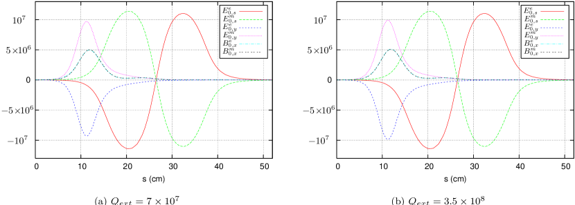
Figure 2: Field profiles of MWS standing waves for $Q_{ext}$ values of $7\times 10^{7}$ and $3.5\times 10^{8}$. Units are MV/m and T for the electric and magnetic fields respectively. $E^{e}_{0,y}$ and $E^{m}_{0,y}$ are scaled by $10^{3}$ and $B^{e}_{0,x}$ and $B^{m}_{0,x}$ are scaled by $10^{9}$. The standing wave approximation is justified with $\mathbf{E}_{0}^{m}\approx-\mathbf{E}_{0}^{e}$ and $\mathbf{B}_{0}^{m}\approx\mathbf{B}_{0}^{e}$

IV.2 Obtaining Realistic $Q_{ext}$ Values

Simulations in MWS were run varying the depth of the inner conductor in order to obtain $Q_{ext}$ values in the vicinity of the proposed value $10^{8}$ Liepe . In order to obtain the high $Q_{ext}$ values it is necessary to raise the inner conductor into the coupler, signified by a negative depth value. The depth used to achieve two high $Q_{ext}$ values are $-9.6$ mm for $Q_{ext}=7\times 10^{7}$ and $-16.4$ mm for $Q_{ext}=3.5\times 10^{8}$. The field profiles along the central cavity axis are shown in Fig. 2. For these calculations the coupler boundary is positioned such that $s^{e}=-1$. From these profiles it is clear that $\mathbf{E}_{0}^{m}\approx-\mathbf{E}_{0}^{e}$ and $\mathbf{B}_{0}^{m}\approx\mathbf{B}_{0}^{e}$ and that therefore the standing wave approximation is justified for these large $Q_{ext}$ values.

V Calculation of Coupler Kick

In this section we present the methods used to calculate a realistic value for the coupler kick. The calculation involves integration of the synthesized field profiles simulated in MWS to get the total, complex change in momentum of one charged particle. In addition we use the standing wave approximation to support analytically our results of emittance growth from simulation of one bunch of electrons through the Cornell ERL.

V.1 Single Cavity

From the synthesized waves along the central cavity axis we can determine the Lorentz force on a particle of charge $q$ traveling down the center of the cavity, at velocity $v$, at each position as a function of time and integrate to obtain the total change in momentum. We begin with examining the kick due to solely inward traveling waves. This calculation is equivalent to a cavity with beam loading with a negligible reflection coefficient:

$$\Delta\mathbf{P}^{+}=q\int_{t_{i}}^{t_{f}}[\mathbf{E}^{+}_{0}(s,t)+v\mathbf{e}_{s}\times\mathbf{B}^{+}_{0}(s,t)]dt,$$ (24)

with $s=vt$. With length $L$ of the cavity we can change the variable of integration to $s$:

$$\Delta\mathbf{P}^{+}=\frac{q}{v}\int_{0}^{L}[\mathbf{E}_{0}^{+}(s,s/v)+v\mathbf{e}_{s}\times\mathbf{B}_{0}^{+}(s,s/v)]ds.$$ (25)

Equation (11) leads to

$$\Delta\mathbf{P}^{+}= e^{i\phi^{+}}\frac{q}{v}\int_{0}^{L}\{[\xi\mathbf{E}^{m}_{0}(s)+i\mathbf{E}^{e}_{0}(s)]$$ (26)

$$+v\mathbf{e}_{s}\times[\mathbf{B}^{e}_{0}(s)+i\xi\mathbf{B}^{m}_{0}(s)]\}e^{-i\omega\frac{s}{v}}ds.$$

From now on, as in the above equation, we will work with complex expressions for the change in momentum of which the real part is physical. For an electron arriving at $s=0$ at a time $\Delta t$ the kick is obtained by replacing $s$ with $s+v\Delta t$ in the exponent of Eq. (26).

The coupler kick $\kappa$ is defined as the ratio of the transverse kick and the longitudinal accelerating kick. Defining our axes such that the transverse kick resides solely in the $y$ direction we have for the coupler kick

$$\kappa^{+}=\frac{\Delta P^{+}_{y}}{\Delta P^{+}_{s}}=\frac{|\Delta P^{+}_{y}|}{|\Delta P^{+}_{s}|}e^{i\phi_{c}}$$ (27)

where

$$\Delta P_{y}^{+}=\frac{e}{c}\int_{0}^{L}[E_{0,y}^{+}(s,s/c)+cB_{0,x}^{+}(s,s/c)]ds$$ (28)

and

$$\triangle P_{s}^{+}=\frac{e}{c}\int_{0}^{L}E_{0,s}^{+}(s,s/c)ds.$$ (29)

V.2 Effect due to Alternating Position of Coupler

In the MWS simulations the coupler is situated in front of the cavity. However, in configurations (af) and (aa) the coupler will alternate from being placed in front of and behind the cavity. It is therefore necessary to model the change in momentum due to a coupler kick supplied after the particle exits the cavity. We find that the same MWS field profiles from the simulations with the coupler in front of the cavity can be used for this second calculation. The transverse fields with the alternate position of the coupler can be modeled by taking the mirror image of the original fields, negating the magnetic field so as to ensure the traveling wave in the coax satisfies Maxwell’s equations. From Eq. (26) the subsequent transverse and longitudinal kicks can be written as

$$\Delta\mathbf{P}_{\bot}^{\prime+}=e^{i\phi^{+}}\frac{q}{v}\int_{0}^{L}\{[\xi\mathbf{E}^{m}_{0,\bot}(L-s)+i\mathbf{E}^{e}_{0,\bot}(L-s)]$$ (30)

$$-v\mathbf{e}_{s}\times[\mathbf{B}^{e}_{0,\bot}(L-s)+i\xi\mathbf{B}^{m}_{0,\bot}(L-s)]\}e^{-i\omega\frac{s}{v}}ds$$

and

$$\Delta P_{s}^{\prime+}=-e^{i\phi^{+}}\frac{q}{v}\!\int_{0}^{L}\!\![\xi E^{m}_{0,s}(L-s)+iE^{e}_{0,s}(L-s)]e^{-i\omega\frac{s}{v}}ds.$$ (31)

A change of variables from $s$ to $L-s$ leads to

$$\Delta\mathbf{P}_{\bot}^{\prime+}= e^{i\phi^{+}}\frac{q}{v}\int_{0}^{L}\{[\xi\mathbf{E}^{m}_{0,\bot}(s)+i\mathbf{E}^{e}_{0,\bot}(s)]$$ (32)

$$-v\mathbf{e}_{s}\times[\mathbf{B}^{e}_{0,\bot}(s)+i\xi\mathbf{B}^{m}_{0,\bot}(s)]\}e^{i\omega\frac{s-L}{v}}ds$$

and

$$\Delta P_{s}^{\prime+}=-e^{i\phi^{+}}\frac{q}{v}\!\int_{0}^{L}\!\![\xi E^{m}_{0,s}(s)+iE^{e}_{0,s}(s)]e^{i\omega\frac{s-L}{v}}ds.$$ (33)

We now compare the coupler kicks due to the two different positions of the coupler, starting with the expressions for change in momentum of Eqs. (26), (32) and (33). We will restrict the analysis to highly relativistic particles. Making the substitutions of Eq. (16), the expression for the change in momentum of Eq. (26) simplifies to

$$\Delta\mathbf{P}^{+} \approx(\xi+is^{e})e^{i\phi^{+}}\frac{q}{c}\int_{0}^{L}\{\mathbf{E}^{m}_{0}(s)\hskip 56.9055pt$$ (34)

$$\hskip 85.35826pt+ic\mathbf{e}_{s}\times\mathbf{B}^{m}_{0}(s)\}e^{-i\omega\frac{s}{c}}ds$$

$$\approx A\mathbf{F}$$

with $A$ defined in Eq. (15). Similarly for Eqs. (32) and (33):

$$\Delta\mathbf{P}_{\bot}^{\prime+} \approx(\xi+is^{e})e^{i\phi^{+}}\frac{q}{c}\int_{0}^{L}\{\mathbf{E}^{m}_{0,\bot}(s)\hskip 56.9055pt$$ (35)

$$\hskip 85.35826pt-ic\mathbf{e}_{s}\times\mathbf{B}^{m}_{0,\bot}(s)\}e^{i\omega\frac{s-L}{c}}ds$$

$$\approx A\mathbf{F}_{\bot}^{*}e^{-i\omega\frac{L}{c}}$$

and

$$\Delta P_{s}^{\prime+} \approx-(\xi+is^{e})e^{i\phi^{+}}\frac{q}{c}\int_{0}^{L}E^{m}_{0,s}(s)e^{i\omega\frac{s-L}{c}}ds$$ (36)

$$\approx-AF_{s}^{*}e^{-i\omega\frac{L}{c}}.$$

Evaluating the coupler kicks through substitution into Eq. (27) leads to cancellation of the constant terms $\xi+is^{e}$ along with the exponential term $e^{-i\omega\frac{L}{c}}$ in the expression for $\Delta P^{\prime+}$. We thus obtain for the two coupler kicks

$$\kappa^{+}\approx\frac{\int_{0}^{L}\{\mathbf{E}^{m}_{0,y}(s)+ic\mathbf{e}_{s}\times\mathbf{B}^{m}_{0,x}(s)\}e^{-i\omega\frac{s}{c}}ds}{\int_{0}^{L}\mathbf{E}^{m}_{0,s}(s)e^{-i\omega\frac{s}{c}}ds}=\frac{F_{y}}{F_{s}}$$ (37)

and

$$\kappa^{\prime+}\approx\frac{\int_{0}^{L}\{\mathbf{E}^{m}_{0,y}(s)-ic\mathbf{e}_{s}\times\mathbf{B}^{m}_{0,x}(s)\}e^{i\omega\frac{s}{c}}ds}{-\int_{0}^{L}\mathbf{E}^{m}_{0,s}(s)e^{i\omega\frac{s}{c}}ds}=-\frac{F^{*}_{y}}{F^{*}_{s}}.$$ (38)

The result of this comparison is the observation that the coupler kick due to the coupler situated at the end of the cavity is the negative complex conjugate of the coupler kick due to a coupler located at the beginning of the cavity:

$$\kappa^{\prime+}\approx-(\kappa^{+})^{*}$$ (39)

We can now calculate the approximate effect on emittance and orbit distortion from two consecutive cavities with the couplers placed before the first cavity and after the second cavity, i.e. configurations (ta) and (aa). For configuration (ta) where both coupler kicks are in the same direction this can be done by adding to Eq. (4) a second similar equation with the coupler phase $\phi_{c}$ changed to $-\phi_{c}+\pi$, from Eq. (39):

$$\Delta y^{\prime} \approx\frac{\Delta E_{0}}{E}|\kappa|\{\cos(\phi_{c}+\psi)-\omega\sin(\phi_{c}+\psi)\Delta t$$ (40)

$$\hskip 28.45274pt+\cos(-\phi_{c}+\psi+\pi)-\omega\sin(-\phi_{c}+\psi+\pi)\Delta t\}$$

$$\approx-2\frac{\Delta E_{0}}{E}|\kappa|\{\sin(\phi_{c})\sin(\psi)+\omega\sin(\phi_{c})\cos(\psi)\Delta t\}.$$

Similarly we can approximate the effect on emittance from the (aa) configuration by instead subtracting the second kick from Eq. (4):

$$\Delta y^{\prime} \approx\frac{\Delta E_{0}}{E}|\kappa|\{\cos(\phi_{c}+\psi)-\omega\sin(\phi_{c}+\psi)\Delta t$$ (41)

$$\hskip 28.45274pt-\cos(-\phi_{c}+\psi+\pi)+\omega\sin(-\phi_{c}+\psi+\pi)\Delta t\}$$

$$\approx 2\frac{\Delta E_{0}}{E}|\kappa|\{\cos(\phi_{c})\cos(\psi)-\omega\cos(\phi_{c})\sin(\psi)\Delta t\}.$$

On crest operation, or $\psi=0$, leads to a cancellation of the $\Delta t$ term in Eq. (41) and thus to no emittance growth with the (aa) configuration, while for the (ta) configuration on crest operation with $\psi=0$ leads to no orbit distortion $\Delta y_{0}^{\prime}$. Other effects that we can deduce from the above two equations are that with off-crest operation, $\psi=\pi$ as in a bunch compressor or a hadron storage ring, there is zero emittance growth with the (ta) configuration and zero orbit distortion with the (aa) configuration.

Coupler kicks were calculated using Eqs. (26) and (32), without assuming standing wave approximation, by numerical integration of the field profiles of MWS in MathCad. The phase of the coupler kicks and the respective magnitudes are shown in Table 2, for both proposed $Q_{ext}$ values and for the two positions of the coupler, before and after the cavity. From the results we see that Eq. (39) holds: the coupler strengths are equivalent for the different positions of the coupler and the coupler phases are are related via $\phi_{c}^{\prime}=-\phi_{c}+\pi$. The position of the coupler boundary in the MWS simulations were chosen such that $\xi=1$ to achieve equivalent accuracies of the electric and magnetic boundary field profiles. We have observed that choosing a coupler boundary position with a very large $\xi$ leads to low accuracy in the electric boundary fields, and choosing a position with a small $\xi$ leads to low accuracy in the magnetic boundary fields.

Table 2: Coupler kick parameters.

	$Q_{ext}=7\times 10^{7}$		$Q_{ext}=3.5u\times 10^{8}$
	Before Cav	After Cav	Before Cav	After Cav
$|\kappa|(10^{-4})$	.9651	.9891	1.039	1.027
$\phi_{c}$ (rad)	2.838	0.349	2.819	0.326

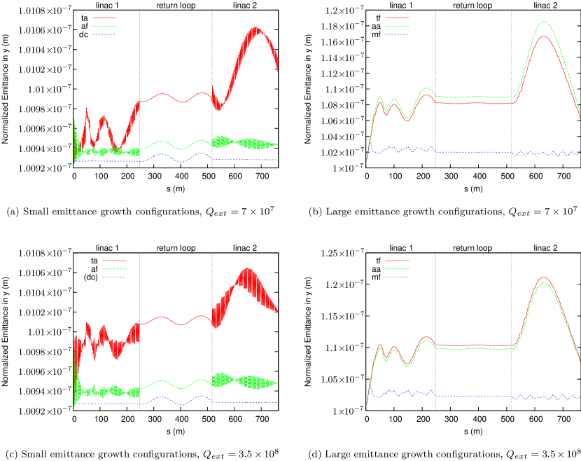
Figure 3: Normalized emittance in the y direction.

Shown in Fig. 3 are results of normalized emittance from simulations in BMAD through the ERL lattice with the calculated coupler kick values for both proposed $Q_{ext}$ values and for all six coupler configurations. The initial normalized emittance is $1\times 10^{-7}$m. The Cornell ERL is split into two accelerating sections, labeled as linac 1 and 2, connected by a return loop hoffstaetter07_1 . To compensate for overall transverse kicks, the necessary corrector coil strengths are computed and included in the lattice.

As one might expect from our previous conclusion, the increase in normalized emittance is small for the (aa) and (af) configurations while large for the (ta) configuration which has a nearly identical effect as the (tf) configuration. Hence, these $Q_{ext}$ values of $7\times 10^{7}$ and $3.5\times 10^{8}$ are large enough to sufficiently satisfy the standing wave approximation. We have found that $Q_{ext}$ values in the vicinity of $10^{5}$, such as for the ERL injector cavities, do not satisfy the standing wave approximation well enough and the emittance growth is not sufficiently small for the (aa) configuration. In our experience, the standing wave approximation holds sufficiently well for $Q_{ext}$ values greater than $10^{7}$.

From these results we come to the conclusion that for operating at or near on crest, configuration (aa) is preferable if conservation of emittance is of primary concern. Configuration (ta) is preferable for operating completely off-crest as is apparent after substitution of $\psi=\pi$ into Eq. (40). However, for certain applications minimizing the orbit distortion and hence the overall transverse kick is of importance. From Eqs. (40) and (41) we see that the (ta) configuration results in less of a transverse orbit distortion than does the (aa) configuration with on crest operation and may be a preferable configuration than the (aa) configuration in certain applications.

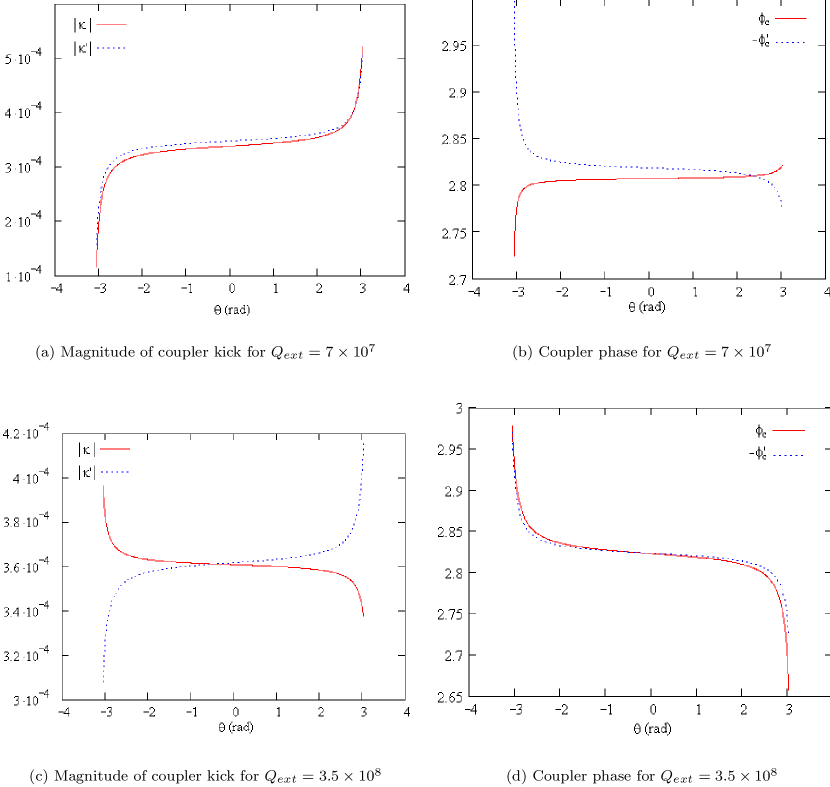
Figure 4: Coupler kick for couplers situated before and after the cavity, the latter signified by a prime, as functions of the phase difference $\theta$ between incoming and reflected waves.

V.3 Reflected Waves in the Cavity

In many applications cavities are operated with large reflection of the incoming RF wave. For example, in an ERL, for which there are an equal number of accelerating bunches as there are decelerating bunches, beam loading can be neglected and the incoming energy is not transferred to the beam in steady state operation. Because the value of $Q_{0}$ is large compared to that of $Q_{ext}$ inside the superconducting cavities, nearly all of the incoming energy will be reflected in RF waves traveling back up the coupler. Both the incoming and the outgoing waves will excite standing waves in the cavity. These standing waves will differ by a phase factor $\phi$ determined by the cavity detuning, with a phase difference of zero for on resonance operation. The amplitudes will be equal for full reflection. It is necessary to examine the coupler kick due to a superposition of incoming and outgoing waves and to determine whether the result of Eq. (39), namely the cancellation of emittance growth due to alternating the coupler from front to back of the cavity, still holds for arbitrary phase differences and different detuning of adjacent cavities.

Due to the reflected waves, in addition to ${\bf\Delta P^{+}}$ there will be kicks:

$$\Delta\mathbf{P}^{-} =\frac{q}{v}\int_{0}^{L}[\mathbf{E}_{0}^{-}(s,s/v)+v\mathbf{e}_{s}\times\mathbf{B}_{0}^{-}(s,s/v)]ds$$ (42)

$$=e^{i\phi^{-}}\frac{q}{v}\int_{0}^{L}\{[\xi\mathbf{E}^{m}_{0}(s)-i\mathbf{E}^{e}_{0}(s)]$$

$$\hskip 11.38109pt-v\mathbf{e}_{s}\times[\mathbf{B}^{e}_{0}(s)-i\xi\mathbf{B}^{m}_{0}(s)]\}e^{-i\omega\frac{s}{v}}ds$$

with the coupler situated in front of the cavity and

$$\Delta\mathbf{P^{\prime}}_{\bot}^{-}=e^{i\phi^{-}}\frac{q}{v}\int_{0}^{L}\{[\xi\mathbf{E}^{m}_{0,\bot}(s)-i\mathbf{E}^{e}_{0,\bot}(s)]$$ (43)

$$\hskip 11.38109pt+v\mathbf{e}_{s}\times[\mathbf{B}^{e}_{0,\bot}(s)-i\xi\mathbf{B}^{m}_{0,\bot}(s)]\}e^{i\omega\frac{s}{v}}e^{-i\omega\frac{L}{v}}ds$$

and

$$\Delta{P^{\prime}}_{s}^{-}=-e^{i\phi^{-}}\frac{q}{v}\int_{0}^{L}[\xi E^{m}_{0,s}(s)-iE^{e}_{0,s}(s)]e^{i\omega\frac{s}{v}}e^{-i\omega\frac{L}{v}}ds.$$ (44)

for the coupler situated after the cavity. Making the substitutions of Eq. (16) and setting $v=c$ for highly relativistic particles leads to:

$$\Delta\mathbf{P}^{-} \approx(\xi-is^{e})e^{i\phi^{-}}\frac{q}{c}\int_{0}^{L}\{\mathbf{E}^{m}_{0}(s)\hskip 56.9055pt$$ (45)

$$\hskip 85.35826pt+ic\mathbf{e}_{s}\times\mathbf{B}^{m}_{0}(s)\}e^{-i\omega\frac{s}{c}}ds$$

$$\approx A\mathbf{F}$$

and

$$\Delta\mathbf{P}_{\bot}^{\prime-} \approx(\xi-is^{e})e^{i\phi^{-}}\frac{q}{c}\int_{0}^{L}\{\mathbf{E}^{m}_{0,\bot}(s)\hskip 56.9055pt$$ (46)

$$\hskip 85.35826pt-ic\mathbf{e}_{s}\times\mathbf{B}^{m}_{0,\bot}(s)\}e^{i\omega\frac{s-L}{c}}ds$$

$$\approx A\mathbf{F}_{\bot}^{*}e^{-i\omega\frac{L}{c}}$$

and

$$\Delta P_{s}^{\prime-} \approx-(\xi-is^{e})e^{i\phi^{-}}\frac{q}{c}\int_{0}^{L}E^{m}_{0,s}(s)e^{i\omega\frac{s-L}{c}}ds$$ (47)

$$\approx-AF_{s}^{*}e^{-i\omega\frac{L}{c}}.$$

The coupler kick $\kappa(\alpha)$, including these reflected waves, is thus given by

$$\kappa(\alpha)=\frac{\Delta P^{+}_{y}+\alpha\Delta P^{-}_{y}}{\Delta P^{+}_{s}+\alpha\Delta P^{-}_{s}},$$ (48)

where $\Delta\mathbf{P}^{+}$ and $\Delta\mathbf{P}^{\prime+}$ are given in Eqs. (34), (35) and (36) and $\alpha$ is the complex reflection coefficient.

We can now compare the coupler kicks including the reflected waves from a coupler situated in front of the cavity and a coupler situated after the cavity:

$$\kappa(\alpha)\approx\frac{AF_{y}+\alpha AF_{y}}{AF_{s}+\alpha AF_{s}}=\frac{F_{y}}{F_{s}}=\kappa^{+}$$ (49)

and

$$\kappa^{\prime}(\alpha^{\prime})\approx\frac{AF^{*}_{y}+\alpha^{\prime}AF^{*}_{y}}{-AF^{*}_{s}-\alpha^{\prime}AF^{*}_{s}}=\frac{F^{*}_{y}}{-F^{*}_{s}}=\kappa^{\prime+}=-(\kappa^{+})^{*}.$$ (50)

We find that the coupler kick is independent of reflected waves and their phases relative to the incoming waves and thus again the complex conjugate relationship should be valid for arbitrary detuning:

$$\kappa^{\prime}\approx-\kappa^{*}$$ (51)

for any values of $\alpha$ and $\alpha^{\prime}$. Therefore, the orbit distortion from two successive cavities for which the couplers are on different sides of their respective cavities but mounted on the same side of the beam pipe still cancel even with reflection.

Figure 4 plots, for both proposed $Q_{ext}$ values, the phase and amplitude of the coupler kicks as a function of the phase difference between incoming and reflected waves for two adjacent cavities with full reflection, $|\alpha|=1$. As before, the position of the boundary is chosen with $\xi=1$ and $s^{e}=-1$. The phase difference $\theta$ is varied from $-\pi$ to $\pi$ with a phase difference of zero for no detuning. For small detuning, with a phase difference around 0, the negative complex conjugacy approximation is satisfied very well.

VI Alternative Methods for Reducing Coupler-Kick Effect

VI.1 Minimizing Coupler Phase

As illustrated previously, the alternating phase of the coupler kick due to the alternating placement of the coupler leads to low emittance growth and/or lower orbit distortion. An alternative method for minimizing emittance growth which does not depend on the alternating placement of the coupler entails manipulating the coupler kick such that its phase is $0$ or $\pi$. As the change in emittance of Eq. (7) varies with $S^{2}$ and thus with $\sin^{2}(\phi_{c}+\psi)$, operation at $\psi=0$ leads to low emittance growth for $\phi_{c}=0$ or $\pi$. This method reduces the effects from each individual coupler and is effective no matter the configuration of couplers along the lattice.

The coupler kick phase is dependent on the distance the coupler is situated from the entrance of the cavity. In the previous simulations the coupler was positioned 4.5 cm from the entrance of the cavity. We find that moving the coupler out to a distance of 5.3 cm leads to a coupler phase of $\pi$ for $Q_{ext}=7\times 10^{7}$ and moving out to a distance of 5.5 cm leads to a phase of $\pi$ for $Q_{ext}=3.5\times 10^{8}$. The coupler kick parameters are listed in Table 3.

Table 3: Coupler kick parameters with optimized coupler phase.

	$Q_{ext}=7\times 10^{7}$		$Q_{ext}=3.5\times 10^{8}$
	Before Cav	After Cav	Before Cav	After Cav
$|\kappa|$($10^{-4})$	.6037	.6066	.5943	.6043
$\phi_{c}$(rad)	3.126	0.129	3.129	0.042

Figures 5 and 6 show the results of normalized emittance through the ERL lattice for all six coupler arrangements with the coupler parameters of Table 3. The emittance growth is decreased substantially for all cases illustrating the dependence of the emittance growth on the phase of the coupler kick.

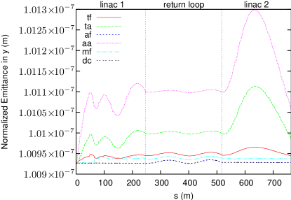
Figure 5: Normalized emittance in the y direction for the six coupler configurations for $Q_{ext}=7\times 10^{7}$.

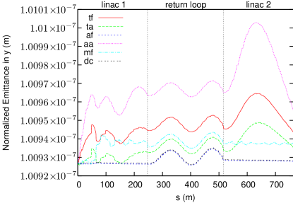
Figure 6: Normalized emittance in the y direction for the six coupler configurations for $Q_{ext}=3.5\times 10^{8}$.

VI.2 Symmetrizing Stub

The above methods for reducing emittance growth, namely the alternating position of the coupler as in configuration (aa) and the phase minimization technique, all depend on operation on crest, $\psi=0$. For certain applications it is preferable to operate slightly off crest. For such applications an alternative method for reducing emittance growth is adding a stub across from the coupler as illustrated in Fig. 7. The stub is used to minimize the asymmetry in the beam pipe causing the transverse fields in the coupler region. The method reduces amplitudes of the off axis fields and thus reduces the magnitude of the coupler kick depending on the depth of the stub, a larger stub leading to lower off axis field amplitudes.

Simulations were run with configuration (aa) $9^{\circ}$ off crest with the coupler placed 4.5 cm from the entrance of the beam pipe, i.e. phase not minimized, to investigate the extent of the dependence of the emittance growth cancellation on $\psi$. A second simulation was run with the same configuration, $\psi=9^{\circ}$, but with a stub of only 1 cm depth added to the cavity. The 1 cm depth is not the result of an optimization but is chosen small enough so as to illustrate the effectiveness of the symmetrizing stub. Larger stub depths did not result in less emittance growth.

As illustrated in Fig. 8, the emittance growth with no stub is significantly larger than the previous, on crest simulations, Fig. 3, illustrating the dependence on $\psi$. The addition of the only 1cm long stub eliminates emittance growth through the two linacs very effectively. The emittance increase in the return loop between linacs is independent of the coupler kicks.

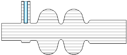
Figure 7: Accelerating cavity with 1 cm symmetrizing stub.

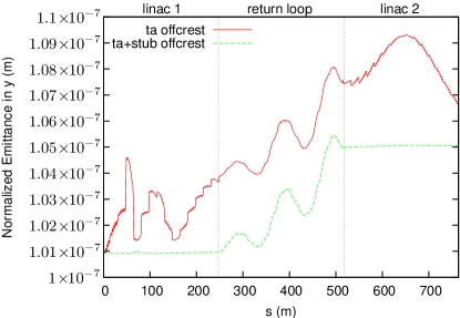
Figure 8: Emittance growth with off crest operation with and without symmetrizing stub.

VII Conclusion

We have investigated three methods of minimizing the emittance growth due to coupler kicks in linacs: (a) alternating the position and direction of the coupler each cavity, (aa) configuration, (b) Choosing the distance between coupler and cavity to minimize the coupler kick for on crest acceleration, (c) symmetrizing the coupler region by adding a stub opposite the coupler. All three methods are shown to work very well. For (a) we find that it is necessary to implement the more technically challenging configuration of alternating the side of the beam pipe the coupler is mounted each cavity. However, we find that for techniques (b) and (c) the one-sided coupler configurations (tf) and (ta) lead to sufficiently low emittance growth. For technique (c) it is interesting to note that a very small symmetrizing stub of only 1 cm can suppress emittance growth very well., independent of the acceleration phase. In addition, method (c) produces very small orbit distortions, similar to configuration (ta) and (af) which do not have small emittance growth.

References

- (1) M. Zhang and Ch. Tang, Beam Dynamics of the Tesla Power Coupler, PAC99, New York/NY (1999)
- (2) M. Dohlus, The Influence of the Main-Coupler Field on the Transverse Emittance of a Superconducting RF Gun, EPAC04, Lucerne/CH (2004)
- (3) S. Belomestnykh, M. Liepe, H. Padamsee, V. Shemelin and V. Veshcherevich, High Average Power Fundamental Input Couplers for the Cornell University ERL: Requirements, Design Challenges and First Ideas, Report ERL 02-8 (2002)
- (4) V. Shemelin, S. Belomestnykh, H. Padamsee, Low-Kick Twin-Coaxial and Waveguide-Coaxial Couplers for ERL, Cornell University Report SRF 021028-08 (2002)
- (5) Z. Greenwald and D. L. Rubin, Emittance Growth Study Using 3DE Code for the ERL Injector Cavities with Various Coupler Configurations, Cornell University Report ERL 03-09 (2003)
- (6) V. Shemelin, S. Belomestnykh, R.L. Geng, M. Liepe. H. Padamsee, Dipole-Mode-Free and Kick-Free 2-Cell Cavity for the SC ERL injector, in Proceedings PAC03 Portland/OR (2003)
- (7) CST Microwave Studio, User Guide, CST GmbH, Budinger Str. D-64289 Darmstadt, Germany (2007)
- (8) D. Sagan, BMAD Manual
- (9) M. Dohlus and S. G. Wipf, Numerical Investigation of Waveguide Input Couplers for the Tesla Superstructure, EPAC00, Vienna/At (2000)
- (10) W. Hartung and E. Haebel, Search of trapped modes in the single-cell cavity prototype for CESR-B, PAC93, Washington DC (1993)
- (11) P. Balleyguier, External Q Studies for APT SC-Cavity Couplers, LINAC’98 Chicago, IL (1998)
- (12) P. Balleyguier, Particle Accelerators, v. 57, pp. 113-127 (1997)
- (13) V. Shemelin, S. Belomestnykh, Calculation of the B-cell cavity external Q with MAFIA and Microwave Studios, Cornell University LNS report SRF 020620-03 (2002)
- (14) N. Kroll, Computer Determination of the External Q and Resonant Frequency of Waveguide Loaded Cavities Particle Accelerators, v. 34, p. 234 (1990)
- (15) M. Liepe, S. Belomestnykh, J. Dobbins, R. Kaplan, C. Strohman, B. Stuhl, C. Hovater, T. Plawski, Pushing the Limits: RF Field Control at High Loaded Q, PAC05, Knoxville/TN (2005)
- (16) G.H. Hoffstaetter, I.V. Bazarov, D.H. Bilderback, J. Codner, B. Dunham, D. Dale, K. Finkelstein, M. Forster, S. Greenwald, S.M. Gruner, Y. Li, M. Liepe, C. Mayes, D. Sagan, C.K. Sinclair, C. Song, A. Temnykh, M. Tigner, Y. Xie, Proceedings PAC07, Albuquerque/NM (2007)
- (17) Controlling coupler-kick emittance growth in the Cornell ERL main linac G.H. Hoffstaetter, B. Buckley, Proceedings PAC07, Albuquerque/NM (2007)