On the stabilization of ion sputtered surfaces

Abstract

The classical theory of ion beam sputtering predicts the instability of a flat surface to uniform ion irradiation at any incidence angle. We relax the assumption of the classical theory that the average surface erosion rate is determined by a Gaussian response function representing the effect of the collision cascade and consider the surface dynamics for other physically-motivated response functions. We show that although instability of flat surfaces at any beam angle results from all Gaussian and a wide class of non-Gaussian erosive response functions, there exist classes of modifications to the response that can have a dramatic effect. In contrast to the classical theory, these types of response render the flat surface linearly stable, while imperceptibly modifying the predicted sputter yield vs. incidence angle. We discuss the possibility that such corrections underlie recent reports of a “window of stability” of ion-bombarded surfaces at a range of beam angles for certain ion and surface types, and describe some characteristic aspects of pattern evolution near the transition from unstable to stable dynamics. We point out that careful analysis of the transition regime may provide valuable tests for the consistency of any theory of pattern formation on ion sputtered surfaces.

I Introduction

Uniform ion beam sputter erosion of a solid surface often causes a spontaneously-arising topographic pattern in the surface topography Navez et al. (1962); Carter et al. (1977); Lewis et al. (1980); Bradley and Harper (1988); Malherbe (1994); Mayer et al. (1994); Chason et al. (1994); Cuerno and Barabasi (1995); Carter and Vishnyakov (1996); Makeev and Barabasi (1997); Facsko et al. (1999); Judy et al. (1999); Erlebacher et al. (1999, 2000); Facsko et al. (2001); Flamm et al. (2001); Habenicht (2001); Costantini et al. (2001); Umbach et al. (2001); Valbusa et al. (2002); Makeev et al. (2002); Chason and Aziz (2003); Facsko et al. (2004); Castro et al. (2005); Chan and Chason (2005); Cuenat et al. (2005); Feix et al. (2005); Rusponi et al. (1997); Brown and Erlebacher (2005); Brown et al. (2005); Ziberi et al. (2005, 2006); Aziz (2006), that can take the form of a one-dimensional corrugation or a two-dimensional array of dots with typical length scales of $10^{2\pm 1}$ nm. Periodic self-organized patterns with wavelength as small as 15 nm Mayer et al. (1994); Facsko et al. (2001) have stimulated interest in this method as a means of nanofabrication at sub-lithographic length scales Cuenat et al. (2005). Because the characteristic scale of the patterns can be three orders of magnitude larger than the characteristic penetration depth of ions into a solid surface, the patterns result from a nontrivial interplay between the sputter erosion on one hand and surface relaxation mechanisms on the other hand.

The present understanding of sputter morphology evolution originates in the Sigmund theory of sputtering Sigmund (1969). Sigmund posited that the local erosion rate of the surface is proportional to the local atom emission rate resulting from the atomic collision cascade, and that the emission rate at a point on the surface is proportional to the nuclear energy deposition density at that point resulting from collision cascades from the ions impinging at all points. Sigmund subsequently Sigmund (1973) recognized the destabilizing influence of the curvature-dependence of the sputter yield (atoms out per incident ion) by modeling the nuclear energy deposition density as taking the form of Gaussian ellipsoids beneath the surface and showing that, as a consequence, concave regions of the surface receive more energy and thereby erode more rapidly than do convex regions .

The origin of the characteristic length scale of the self-organized patterns was identified by Bradley and Harper (BH) Bradley and Harper (1988), who recognized that Sigmund’s destabilization mechanism is opposed by surface diffusion, which operates so as to return the surface to flatness. Expanding Sigmund’s Gaussian ellipsoid response in powers of derivatives of the surface height $h(x,y,t)$ and superposing classical Mullins-Herring Herring (1950); Mullins (1959) surface diffusion, BH derived a linear partial differential equation (PDE) Bradley and Harper (1988) that describes the evolution of the surface height on scales much larger than the characteristic length scales of Sigmund’s Gaussian response:

$$\frac{\partial h}{\partial t}=-I+\{S_{x}\partial_{xx}+S_{y}\partial_{yy}-B\nabla^{4}\}h\ ,$$ (1)

where $I(b)$ is the vertical erosion rate of a flat surface, $S_{x}(b)$ and $S_{y}(b)$ are the curvature coefficients, $b$ is the surface slope, and $B$ is a material parameter describing relaxation and containing the surface diffusivity and the surface free energy. The coefficients $I,S_{x}$, and $S_{y}$ are expressed in terms of Sigmund’s Gaussian and depend on $\theta=\tan^{-1}(b)$, the angle between the beam direction, henceforth denoted as $-\hat{z}$, and the local normal to the surface $\hat{n}$ ($0\leq\theta\leq\pi/2$). For nonzero $\theta$, we denote by $\hat{x}$ the axis perpendicular to $\hat{z}$ in the $\hat{n}-\hat{z}$ plane. Bradley-Harper’s linear stability analysis yields unstable modes whenever $S_{x}$ or $S_{y}$ is negative, whose characteristic length scale arises from a balance between the destabilizing effect of the second derivatives $\partial_{xx},\partial_{yy}$ and the stabilizing effect of the surface diffusion term $\nabla^{4}$. The behavior of $S_{x}(\theta)$ and $S_{y}(\theta)$ for characteristic parameter values are shown in Fig. 1.

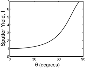
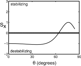
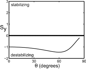
Figure 1: (a) Plot of sputter yield curve $I(\theta)$, normalized by $I(0)$ (b,c) Plots of $S_{x}(\theta)$ and $S_{y}(\theta)$, normalized by $|S_{x}(0)|=|S_{y}(0)|$. The parameters used are: $a=1.5$ nm, $\sigma=0.9$ nm, $\mu=0.5$ nm.

The Bradley-Harper analysis gives rise to the following predictions: (i) Below a crossover angle $\theta_{cross}$, $S_{x}<S_{y}<0$, implying a faster growth rate for parallel mode (wave vector parallel to projected ion beam direction along the surface) than for perpendicular mode (wave vector along $\hat{y}$) surface modulations ; (ii) $S_{y}<0$ for all $\theta$, implying instability to perpendicular modes at all incidence angles. For $\theta>\theta_{cross}$ the perpendicular modes are the fastest to grow with dominant wavelength $\sqrt{8\pi^{2}B/(-S_{y})}$. The generalization of the BH analysis to the nonlinear regime, which is required to account for the observed saturation of ripple amplitude and the emergence of more complicated patterns (e.g. hexagons, dots, pits) was carried out by Cuerno and coworkers Makeev et al. (2002); Cuerno and Barabasi (1995) who expanded Sigmund’s Gaussian ellipsoid model to higher order in surface height derivatives, resulting in a Kuramoto-Sivashinsky type equation Cross and Hohenberg (1993) for the surface evolution.

There is growing evidence that although the Bradley-Harper predictions explain some features of experiments (e.g. the temperature dependence of the wavelength of the ripples Erlebacher et al. (1999)), there are also some glaring inconsistencies. This is clearly demonstrated in, e.g., the recent work of Ziberi et al. Ziberi et al. (2005), who found a “window of stability” for Si surfaces at room temperature bombarded by $\sim 1-2$ keV noble gas ions at an intermediate range of angles $\theta_{1}<\theta<\theta_{2}$, where $\theta_{1}\approx 30^{o}$, and $\theta_{2}\approx 60^{o}$. Moreover, Ziberi et al. demonstrated that when bombarded by some noble ions (${\rm Ne^{+}}$), a flat surface remains stable at all angles. In addition to the experimental inconsistencies with BH prediction (ii), there have also been recent experiments Costantini et al. (2001); Yamada et al. (2001) and atomistic simulations Bringa et al. (2001); Kalyanasundaram et al. (2007) that have measured the shape change of a smooth solid surface in the vicinity of an impingement by a single energetic monatomic ion or cluster ion. These studies show significant deviations from the predictions of Sigmund’s ellipsoidal Gaussian form. For example, the molecular dynamics studies of Feix et al. Feix et al. (2005) indicate that for 5 keV ${\rm Cu^{+}}$ bombardment of Cu crystals, the collision cascade intensity along the surface has a maximum along an annulus some distance from the impact point and its spatial decay is better characterized by an exponential rather than by a Gaussian function. In this case Feix et al. still found linear instability of a flat surface. Moreover, in many cases Costantini et al. (2001); Bringa et al. (2001), including low energy (0.5 keV) bombardment of an amorphous silicon surface Kalyanasundaram et al. (2007), the response of the surface is the formation of craters with rims. This type of response, involving the accumulation of matter at some locations, is in clear contradiction to the purely erosive response predicted by Sigmund’s model using a Gaussian ellipsoid collision cascade. The occurrence of craters with rims has been attributed to thermal spikes Bringa et al. (2001) or to ion-stimulated surface mass transport Kalyanasundaram et al. (2007).

These observations raise the interesting question of how robust are the predictions of BH to the precise shape of the local response to an ion impact. Indeed, the most general evolution equation based on the accumulation of local responses to ion impacts is Aziz (2006)

$$\frac{\partial h({\bf x},t)}{\partial t}=\int{\bf dx^{\prime}}J_{ion}({\bf x^{\prime}})\Delta[{\bf x-x^{\prime}},h_{x}({\bf x},t),h_{y}({\bf x},t),h_{xx}({\bf x},t),h_{yy}({\bf x},t),h_{xy}({\bf x},t),...]\ ,$$ (2)

where ${\bf x}=(x,y)$, $J_{ion}({\bf x^{\prime}})$ is the ion flux at ${\bf x^{\prime}}$, subscripts $x$ and $y$ denote partial derivatives, and the kernel $\Delta[{\bf x-x^{\prime}},\dots]$, representing the change in height at ${\bf x}$ due to an ion impact at ${\bf x^{\prime}}$, is expected to decay smoothly to zero at large distances $|{\bf x}-{\bf x^{\prime}}|$. This equation is more general than that assumed by Sigmund because the kernel $\Delta$ can have any shape whatsoever, and can depend on the complete local geometry of the surface.

In this paper we explore whether a more general physically motivated surface response can change the predictions for linear stability from those of Bradley and Harper. Our purpose here is not to perform quantitative comparison between theory and specific experiments, but rather to determine how robust the predictions of the Bradley-Harper theory are with respect to modifications of the ion impact function $\Delta$. We demonstrate that, whereas the fundamental prediction concerning the instability of flat surface to uniform ion irradiation results from a wide class of response functions including Gaussian and non-Gaussian distributions – thus explaining the applicability of Bradley-Harper theory for wide range of systems – there are certain classes of modification that have a dramatic effect. Notably, these modifications render the flat surface stable – in contradiction to the classical theory – while imperceptibly affecting the yield curve $I(b)$.

The paper is organized as follows: In section II we extend the BH approach – of deriving from the microscopic response function the coefficients $S_{x}(b),S_{y}(b)$ in Eq. (1) – to a broad class of purely erosive surface response functions, of which the Gaussian ellipsoid is a particular example and the response of Feix et al. Feix et al. (2005) is another example. We show that the BH prediction of linear surface instability for all incident beam angles is unchanged. Hence any purely erosive surface response within this broad class is contradicted by experiments. In the remainder of the paper we explore possible physical mechanisms that could resolve this condundrum. In section III, we demonstrate that a surface response that is not purely erosive, but rather consists of the formation of a crater surrounded by a rim, does allow linear stability for some range of incidence angles. In section IV, we demonstrate that impact-induced “downhill” surface currents, such as those recently found in MD simulation of C and Si surfaces bombarded by low energy ($\sim 250$ keV) ions Moseler et al. (2005), can also yield linear stability for some range of beam angles. There are thus multiple physical mechanisms that could explain the experiments, and the essential question is to determine which effect is dominant. Identifying the dominant physical mechanism for linear (in)stability is critical to having a reliable nonlinear theory for pattern formation. In section V, we discuss how experiments might distinguish the competing theories. In particular we argue for a careful analysis of experiments near the observed critical angle at which a flat surface becomes stable.

II Bradley-Harper theory revisited

The Sigmund theory of sputtering Sigmund (1969) posits that the local erosion of the surface in Eq. (2), $\Delta[{\bf x-x^{\prime}}]/\sqrt{1+b^{2}}$ with $b$ the local surface slope, is proportional to the local atom emission rate resulting from the nuclear collision cascade, which itself is proportional to the nuclear energy deposition density at $({\bf x},h({\bf x}))$ from an ion impinging at $({\bf x^{\prime}},h({\bf x^{\prime}}))$. To demonstrate the source of an instabilitySigmund (1973), Sigmund modeled the collision cascade as a Gaussian ellipsoid. Bradley and Harper’s subsequent expansion of Sigmund’s Gaussian ellipsoid collision cascade model, combined with smoothening by fourth-order Mullins-Herring surface diffusion, leads to Eq. (1).

To examine the consequences of forms of the erosive response that are more general than Gaussian ellipsoids, we assume:

$$\Delta[{\bf x-x^{\prime}},\dots] = \Delta h(r,z)$$ (3)

$$= -{A}e^{-g(r)-f(z)}\ ,$$

where $r=\sqrt{x^{2}+y^{2}}$, $z=h(x,y)$, and ${A}$ is a length that depends on parameters such as ion energy and ion and target mass. The first equality in Eq. (3) assumes radial symmetry about the ion track and no explicit dependence on the surface slope and curvature, with the kernel depending only on $r$ and $z$. The second equality assumes separation of the variables $r$ and $z$. In Eq. (3) the ion is assumed to penetrate the surface at $(r,z)=(0,0)$.

Sigmund’s Gaussian ellipsoid response is a particular case of Eq. (3), with

$$f(z)=\frac{1}{2\sigma^{2}}(z-a)^{2}\ \ ;\ \ g(r)=\frac{1}{2\mu^{2}}r^{2}\ ,$$ (4)

where $a$ is the average penetration depth of the ion, and $\sigma$, $\mu$ are lengths characterizing the ranges of response in directions parallel and perpendicular to $\hat{z}$, respectively.

Following Bradley-Harper, we substitute in Eq. (2) the response form (3) and add a relaxation mechanism to the surface dynamics associated with Herring-Mullins surface diffusion:

$$\frac{\partial h}{\partial t}=-B\nabla^{4}h-\alpha\int_{-\infty}^{\infty}\!\!dy\int_{-\infty}^{\infty}\!\!dx\ e^{-g(\sqrt{x^{2}+y^{2}})-f(h(x,y))},$$ (5)

where $\alpha=AJ_{ion}$ and the materials parameter $B$ is given by $B=\gamma\Omega^{2}DC/(k_{B}T)$. Here $C$, $D$, and $\Omega$ are the concentration, diffusivity, and volume, respectively of the surface-diffusing species; $\gamma$ is the surface free energy, $k_{B}$ is Boltzmann’s constant and $T$ is the absolute temperature.

To study evolution of surface morphology in the limit that the surface height $h(x,y,t)$ varies on scales much larger than the ion penetration depth, we consider perturbations about a planar surface $(x,y,h=bx)$, so that

$$h(x,y)=bx+\frac{1}{2}h_{xx}x^{2}+\frac{1}{2}h_{yy}y^{2}+h_{xy}xy+\cdots\ ,$$

and expand $e^{-f(h(x,y))}$ to obtain

$$\exp[-f(h(x,y))]\approx e^{-f(bx)}[1-f^{\prime}(bx)[\frac{1}{2}h_{xx}x^{2}+\frac{1}{2}h_{yy}y^{2}+h_{xy}xy]]\ .$$ (6)

With the expansion (6), the integral equation (5) is readily transformed into the PDE (1) with the coefficients:

$$I(b) = \alpha\int_{-\infty}^{\infty}\!\!dy\int_{-\infty}^{\infty}\!\!dx\ e^{-\rho_{b}(x,y)}$$

$$S_{y}(b) = \alpha\int_{-\infty}^{\infty}\!\!dy\int_{-\infty}^{\infty}\!\!dx\ e^{-\rho_{b}(x,y)}f^{\prime}(bx)y^{2}$$

$$S_{x}(b) = \alpha\int_{-\infty}^{\infty}\!\!dy\int_{-\infty}^{\infty}\!\!dx\ e^{-\rho_{b}(x,y)}f^{\prime}(bx)x^{2}$$ (7)

where $\rho_{b}(x,y)=g(\sqrt{x^{2}+y^{2}})+f(bx)$.

The question now is how various choices of $f(r)$ and $g(z)$ can change $I(b),\ S_{x}(b)$ and $S_{y}(b)$. We are primarily interested in the slope dependence in $S_{y}(b)$, because in the Bradley-Harper theory $S_{y}(b)<0$ for all slopes $b$. Our question is whether any choice of $f(z),g(r)$ can stabilize the surface against perpendicular modes ($S_{y}>0$) for some range of $b$ while not significantly affecting the shape of the yield curve. The latter requirement is especially significant because the yield curve predicted by the Sigmund response function agrees qualitatively with that measured on many materials – at least for non-grazing incidence Vasile et al. (1999).

All of our analysis proceeds with the same methodology: the integral for $S_{y}(b)$ in Eq. (II) is dominated by contributions near the minimum of $\rho_{b}$ which we call $\{x_{min},y_{min}\}$. This is because the size of the region where energy is deposited (of order the penetration depth $a$) is much smaller than the characteristic length scale over which the surface shape varies. The minima of $\rho_{b}$ satisfy the equations

$$\frac{y_{min}}{\sqrt{x_{min}^{2}+y_{min}^{2}}}g^{\prime}(\sqrt{x_{min}^{2}+y_{min}^{2}}) = 0;$$ (8)

$$\frac{x_{min}}{\sqrt{x_{min}^{2}+y_{min}^{2}}}g^{\prime}(\sqrt{x_{min}^{2}+y_{min}^{2}})+bf^{\prime}(bx_{min}) = 0.$$ (9)

Depending on the functional forms of $g$ and $f$ there are two possible types of solutions to these equations.

$${\emph{(}a)} \ \ y_{min}=0,\ \pm g^{\prime}(x_{min})+bf^{\prime}(bx_{min})=0$$ (10)

$${\emph{(}b)} g^{\prime}(\sqrt{x_{min}^{2}+y_{min}^{2}})=0,\ bf^{\prime}(bx_{min})=0\ ,$$ (11)

where the $\pm$ signs in (10) correspond to $x_{min}>0,x_{min}<0$, respectively. Once the locations of the minima are determined, we can expand

$$\rho_{b} = \rho_{b}(x_{min},y_{min})+\frac{(x-x_{min})^{2}}{2}(g_{xx}+b^{2}f^{\prime\prime})$$ (12)

$$+ (x-x_{min})(y-y_{min})g_{xy}+\frac{(y-y_{min})^{2}}{2}g_{yy}$$

$$\equiv \rho^{*}+\tilde{A}(x-x_{min})^{2}+\tilde{C}(x-x_{min})(y-y_{min})+\tilde{B}(y-y_{min})^{2}$$

where the second equality defines $\tilde{A},\tilde{B},\tilde{C},\rho^{*}$. This expansion can then be used to evaluate the integral.

We now proceed to use this methodology to establish the conclusion that $S_{y}\leq 0$ is extremely robust. For any kernel of the form considered here a perpendicular mode instability always exists for all slopes $b$. The characteristic behavior of the coefficient $S_{x}$ is more fickle. Obviously, for $b\to 0$, $S_{x}(b)/S_{y}(b)\to 1$, and therefore $S_{x}(b)$ is necessarily negative for small enough slopes $b$. However, Bradley-Harper’s observation, that Gaussian ellipsoids imply $S_{x}<S_{y}<0$ for $b\ll 1$, does depend on the exact shape of the response function. This can be readily verified by considering Sigmund’s response Eq. (4) with $a<\sigma$. Hence, we will focus our analysis on the robust properties of the linear dynamics, associated with the sign of $S_{y}$, and will not further discuss $S_{x}$ in this section.

II.1 The shape of the energy distribution does not qualitatively affect stability

We begin by considering changes in only the shape of the energy distribution: namely we consider $f(z),g(r)$ that keep the position of maximum energy deposition at a single point (the average stopping point of the ion), though we vary the shape of the distribution. We thus assume that the function $f(z)$ has a minimum at $z=a$ whereas $g(r)$ increases monotonically from $r=0$.

Under these assumptions, the minimum of $\rho_{b}(x,y)$ must be of type (10). Moreover, because the minimum of $g(r)$ along the $x$ axis occurs at $x=0$ and the minimum of $f(bx)$ occurs at $x=a/b>0$, then $x_{min}$, determined by $g^{\prime}(x_{min})+bf^{\prime}(bx_{min})=0$ must be in the interval $0<x_{min}<a/b$, such that $f^{\prime}(bx_{min})<0$. The expansion of $\rho_{b}$ in equation (12) leads to the coefficients $\tilde{A}=(g^{\prime\prime}+b^{2}f^{\prime\prime})/2$, $\tilde{B}=g^{\prime}/2|x_{min}|$ and $\tilde{C}=0$, where all derivatives are taken at $x_{min}$. Hence the integral is approximately

$$S_{y}(b)\approx\alpha\int_{-\infty}^{\infty}\!\!dy\int_{-\infty}^{\infty}\!\!dx\ e^{-\rho^{*}-\tilde{A}(x-x_{min})^{2}-\tilde{B}y^{2}}f^{\prime}(bx_{min})y^{2}.$$ (13)

Because $f^{\prime}(bx_{min})<0$ the integral (13) is necessarily negative for all $b$. This demonstrates that the experimentally observed stability of a sputtered surface to perpendicular mode ripples is not a consequence of the shape of the energy distribution.

II.2 Toroidal energy distributions do not qualitatively affect stability

Another possible modification of the energy distribution is for the maximum energy deposition to occur away from the ion trajectory. Indeed, Feix et al.’s recent simulations of Cu crystals bombarded by 5 keV ${\rm Cu^{+}}$ ions Feix et al. (2005) have demonstrated energy distributions with a maximum along an annulus surrounding the ion trajectory. Such a response is thus characterized by a $g(r)$ with a minimum at $r_{min}=r_{0}>0$.

Consider the sign of $S_{y}(b)$ under these circumstances. There are now two different regimes, depending on the slope. When the slope is small, such that $a/b\geq r_{0}$, the minimum must be of type (a), Eq. (10). Type (b) (Eq. (11)) is excluded because if $f^{\prime}(bx_{min})=0$ then we must have $x_{min}=a/b$. But then the equation $g^{\prime}(r)=0$ cannot be satisfied: this equation implies that $x_{min}^{2}+y_{min}^{2}=r_{0}^{2}$, which cannot be obeyed for any $y_{min}$. In contrast, when the slope is large, so that $a/b\leq r_{0}$, the minima are of type (b).

Let us first consider the regime of small slope. Here the analysis proceeds as above with the same $\tilde{A},\tilde{B},\tilde{C}$ defined in (12). As before the sign of the integral hinges on the value of $f^{\prime}(bx_{min})=-g^{\prime}(x_{min})/b$. Because we are assuming that the minimum of $f(bx)$ occurs at $x=a/b$ which is larger than the minimum assumed by $g(r)$ along the $x$-axis, at $x=r_{0}$, Eq. (10) implies that $f^{\prime}(bx_{min})<0$. Hence we arrive at the conclusion that in the small slope regime $S_{y}\leq 0$: the linear instability survives.

The second regime, where $b/a\leq r_{0}$, is more subtle, with two minima being of type (b) (Eq. 11). Assuming the minimum of $g(r)$ occurs at $r_{0}$, and the minimum of $f(z)$ occurs at $a$, in this case we have that $(x_{min},y_{min}^{\pm})=(a/b,\pm\sqrt{r_{0}^{2}-(a/b)^{2}}).$ The value of $S_{y}(b)$ is given by the sum of the contributions to the integral centered around each of these two minima. For these minima the values of $\tilde{A},\tilde{B},\tilde{C}$ are given by

$$\tilde{A}=\frac{1}{2}\biggl{(}g^{\prime\prime}\frac{x_{min}^{2}}{r_{0}^{2}}+b^{2}f^{\prime\prime}\biggr{)}\ ,\ \tilde{B}=\frac{1}{2}g^{\prime\prime}\frac{y_{min}^{2}}{r_{0}^{2}}\ ,\ \tilde{C}^{\pm}=g^{\prime\prime}\frac{x_{min}y_{min}^{\pm}}{r_{0}^{2}}\ ,$$ (14)

where $g^{\prime\prime}$ is evaluated at $r=r_{0}$ and $f^{\prime\prime}$ is evaluated at $z=a$. We now must evaluate

$$S_{y}(b)\approx\alpha\sum_{\pm}\int_{-\infty}^{\infty}\!\!dy\int_{-\infty}^{\infty}\!\!dx\ e^{-\rho^{*}-\tilde{A}(x-x_{min})^{2}-\tilde{B}(y-y_{min}^{\pm})^{2}-\tilde{C}^{\pm}(x-x_{min})(y-y_{min}^{\pm})}f^{\prime}(bx)y^{2}.$$ (15)

The exponential in the integrals are best dealt with by completing the square, so that they become

$$S_{y}(b)\approx\alpha\sum_{\pm}\int_{-\infty}^{\infty}\!\!dy\int_{-\infty}^{\infty}\!\!dx\ e^{-\rho^{*}-\tilde{A}\biggl{(}(x-x_{min})+\frac{\tilde{C}^{\pm}}{2\tilde{A}}(y-y_{min}^{\pm})\biggr{)}^{2}}e^{-(y-y_{min}^{\pm})^{2}(\tilde{B}-(\tilde{C}^{\pm})^{2}/4\tilde{A})}f^{\prime}(bx)y^{2}.$$ (16)

Now the second exponential decays with $y$ varying away from $y_{min}^{\pm}$ because $\tilde{B}\geq\frac{(\tilde{C}^{\pm})^{2}}{4\tilde{A}}$ for any $b\neq 0$. If we now change variables to ${\tilde{x}}=x-x_{min}+\frac{\tilde{C}^{\pm}}{2\tilde{A}}(y-y_{min}^{\pm})$ and ${\tilde{y}}=y-y_{min}^{\pm}$ we obtain

$$S_{y}(b)\approx e^{-\rho^{*}}\alpha\sum_{\pm}\int_{-\infty}^{\infty}\!\!d{\tilde{y}}\int_{-\infty}^{\infty}\!\!d{\tilde{x}}\ e^{-\tilde{A}{\tilde{x}}^{2}-{\tilde{y}}^{2}(\tilde{B}-(\tilde{C}^{\pm})^{2}/4\tilde{A})}f^{\prime}[b(x_{min}+{\tilde{x}}-\frac{\tilde{C}^{\pm}}{2\tilde{A}}{\tilde{y}})](y_{min}^{\pm}+{\tilde{y}})^{2}\ .$$ (17)

Because now $f^{\prime}(bx_{min})=0$, evaluation of the integrals to leading order requires expansion of the terms $f^{\prime}[b(x_{min}+{\tilde{x}}-\frac{\tilde{C}^{\pm}}{2\tilde{A}}{\tilde{y}})]$ around $a=bx_{min}$. With this we get the following approximation to the integral:

$$S_{y}(b)\approx e^{-\rho^{*}}\alpha\sum_{\pm}\int_{-\infty}^{\infty}\!\!d{\tilde{y}}\int_{-\infty}^{\infty}\!\!d{\tilde{x}}\ e^{-\tilde{A}{\tilde{x}}^{2}-{\tilde{y}}^{2}(\tilde{B}-(\tilde{C}^{\pm})^{2}/4\tilde{A})}\biggl{(}f^{\prime\prime}(a)(b{\tilde{x}}-\frac{\tilde{C}^{\pm}}{2\tilde{A}}b{\tilde{y}})+\cdots\biggr{)}(y_{min}+{\tilde{y}})^{2}.$$ (18)

The contribution of the two integrals is identical, and sums up to:

$$S_{y}(b)\approx-f^{\prime\prime}(a)g^{\prime\prime}(r_{0})\frac{ay_{min}^{2}}{r_{0}^{2}\tilde{A}}\Gamma_{1}$$ (19)

where we have substituted the formula for $C^{\pm}$ (14), have used $bx_{min}=a$, and where

$$\Gamma_{1}=e^{-\rho^{*}}\alpha\int_{-\infty}^{\infty}\!\!d{\tilde{y}}\int_{-\infty}^{\infty}d{\tilde{x}}e^{-\tilde{A}{\tilde{x}}^{2}}e^{-{\tilde{y}}^{2}(\tilde{B}-\tilde{C}^{2}/4\tilde{A})}{\tilde{y}}^{2}\ .$$

The RHS of Eq. (19) is negative definite, i.e. $S_{y}(b)$ is negative for all values of $b$. Hence response functions of the form of Eq. (3) generally cause a perpendicular mode instability for any incidence angle. The qualitative conclusions of the original Bradley-Harper analysis concerning the instability of perpendicular surface modulations at any beam angle are thus very robust.

III Effects of mass redistribution

The analysis of the previous section demonstrates that a broad class of purely erosive response functions gives rise to linear instability for all beam angles. However, there have been several recent studies suggesting that the surface response is not purely erosive. These studies demonstrate that after ion impact, a crater forms around the impact point of the penetrating ion, surrounded by rims elevated from the original surface Bringa et al. (2001); Yamada et al. (2001); Kalyanasundaram et al. (2007); Costantini et al. (2001) . This behavior, where $\Delta h>0$ in the rim, is completely different from the erosive response functions described above. We investigate whether such response functions can cause the stability of a flat surface.

To carry out this analysis, we introduce a natural generalization of the family of response functions (3):

$$\Delta h(r,z)=-\sum A_{j}e^{-g_{j}(r)-f_{j}(z)}$$ (20)

where $g_{j}(r),f_{j}(z)$ are localized functions as discussed in the previous section, but the coefficients $A_{j}$ can be negative or positive. In particular, negative $A_{j}$ corresponds to mass deposition associated with ion impact and can give rise to formation of rims. A particularly simple form of a response function is the sum of two Gaussian ellipsoids:

$$\Delta h(r,z)=-A[e^{-r^{2}/2\mu_{1}^{2}-(z-a_{1})^{2}/2\sigma_{1}^{2}}-\beta e^{-r^{2}/2\mu_{2}^{2}-(z-a_{2})^{2}/2\sigma_{2}^{2}}]\ .$$ (21)

This response function has eight free parameters (including $A$ and $\beta$), all of which are constrained to be positive. Unlike the original Sigmund model, the free parameters here are not directly connected to a microscopic picture. Because our intent is to understand whether small deviations from Sigmund’s response function can change the stability characteristics of the surface, we will consider the case with $\beta\ll 1$, and think of $a_{1},\mu_{1},\sigma_{1}$ as corresponding essentially to the original Sigmund parameters. The parameters $a_{2},\mu_{2},\sigma_{2}$ describe characteristics of the mass redistribution.

With the model so defined, we can evaluate the yield curve $I(b)$ as well as $S_{x}(b),S_{y}(b)$, obtaining

$$I(b) = 2\pi J_{ion}\sum_{i=1,2}A_{i}\mu_{i}^{2}\sigma_{i}\sqrt{\frac{1+b^{2}}{b^{2}\mu_{i}^{2}+\sigma_{i}^{2}}}e^{-a_{i}^{2}/[2(b^{2}\mu_{i}^{2}+\sigma_{i}^{2})]}$$ (22)

$$S_{x}(b) = -2\pi J_{ion}\sum_{i=1,2}A_{i}a_{i}\mu_{i}^{4}\sigma_{i}[b^{2}a_{i}^{2}\mu_{i}^{2}-2b^{4}\mu_{i}^{4}-b^{2}\mu_{i}^{2}\sigma_{i}^{2}+\sigma_{i}^{4}]\sqrt{\frac{1+b^{2}}{(b^{2}\mu_{i}^{2}+\sigma_{i}^{2})^{7}}}e^{-a_{i}^{2}/[2(b^{2}\mu_{i}^{2}+\sigma_{i}^{2})]}$$ (23)

$$S_{y}(b) = -2\pi J_{ion}\sum_{i=1,2}A_{i}a_{i}\mu_{i}^{4}\sigma_{i}\sqrt{\frac{1+b^{2}}{(b^{2}\mu_{i}^{2}+\sigma_{i}^{2})^{3}}}e^{-a_{i}^{2}/[2(b^{2}\mu_{i}^{2}+\sigma_{i}^{2})]}\ ,$$ (24)

where we used the notation $A_{1}=A,A_{2}=-\beta A$.

We now want to use this result to address the following question: is there a regime of parameter space where the stability characteristics of the surface are qualitatively different from the predictions of Bradley and Harper, but for which the yield curve is experimentally indistinguishable from that predicted by the Sigmund response? Indeed, we have found multiple regions of parameter space where this occurs. This can be demonstrated simply and analytically by expanding equations (22,23,24) in the regime of small slopes, where $S_{x}\approx S_{y}$. We find that, as $b\to 0$,

$$I(b) \approx 2\pi J_{ion}A[\mu_{1}^{2}e^{-a_{1}^{2}/(2\sigma_{1}^{2})}-\beta\mu_{2}^{2}e^{-a_{2}^{2}/(2\sigma_{2}^{2})}]$$ (25)

$$S_{y}(b) \approx S_{x}(b)\approx-2\pi J_{ion}A[\frac{a_{1}\mu_{1}^{4}}{\sigma_{1}^{2}}e^{-a_{1}^{2}/(2\sigma_{1}^{2})}-\beta\frac{a_{2}\mu_{2}^{4}}{\sigma_{2}^{2}}e^{-a_{2}^{2}/(2\sigma_{2}^{2})}]\ ,$$ (26)

Here we see that for small slopes, $S_{x}$ and $S_{y}$ can have either sign, depending on the relative magnitudes of the terms $\frac{a_{1}\mu_{1}^{4}}{\sigma_{1}^{2}}e^{-a_{1}^{2}/(2\sigma_{1}^{2})}$ and $\beta\frac{a_{2}\mu_{2}^{4}}{\sigma_{2}^{2}}e^{-a_{2}^{2}/(2\sigma_{2}^{2})}$. If the second term dominates the first then $S_{x}$ and $S_{y}$ are positive at small $b$ and the surface is stable to all perturbations. Can stability be achieved without significantly affecting $I(b)$? Obviously, this will be the case if $\mu_{1}^{2}e^{-a_{1}^{2}/(2\sigma_{1}^{2})}\gg\beta\mu_{2}^{2}e^{-a_{2}^{2}/(2\sigma_{2}^{2})}$. Letting $Z_{i}=\mu_{i}^{2}e^{-a_{i}^{2}/(2\sigma_{i}^{2})}$, satisfaction of the two conditions amounts to finding parameters where (i) $Z_{a}a_{1}\mu_{1}^{2}/\sigma_{1}^{2}<\beta Z_{2}a_{2}\mu_{2}^{2}/\sigma_{2}^{2}$ while (ii) $Z_{1}/Z_{2}\gg\beta$. We also would like $\beta$ to remain small. Such a parameter regime clearly exists and merely constrains the scale and the geometry of the mass redistribution region.

To demonstrate this explicitly, Fig. 2 shows the behavior of $I(b),S_{x}(b),S_{y}(b)$, where we have used the same parameters for $a_{1}=1.5,\sigma_{1}=0.9,\mu_{1}=0.5$ as used for the ’normal’ Bradley-Harper stability characteristics shown in Fig. 1, with the additional parameters $\beta=0.03,\ a_{2}=0.5\textrm{nm,}\ \sigma_{2}=0.5$ nm, and $\mu_{2}=1$ nm. For these parameters $Z_{1}=0.06\textrm{nm}^{2}$ and $Z_{2}=0.6\textrm{nm}^{2}$, thus $Z_{1}/Z_{2}\gg\beta$, whereas $a_{1}\mu_{1}^{2}/\sigma_{1}^{2}=0.46$ nm and $a_{2}\mu_{2}^{2}/\sigma_{2}^{2}=2$ nm. We therefore satisfy both constraints (i) and (ii) listed above. Indeed, the top row of Fig. 2 shows a stable region of parameter space for small slopes in both $S_{x}$ and $S_{y}$, while the qualitative shape of the yield curve is unchanged.

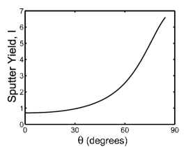
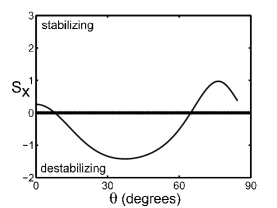
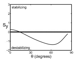
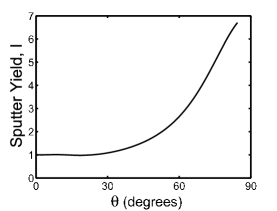
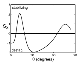
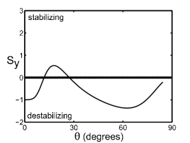
Figure 2: Normalized yield curve and BH coefficients $S_{x},S_{y}$ for two sets of parameters of the two-Gaussians model, Eq. (21). The ”Sigmund parameters” $a,\sigma,\mu$ are taken as in Fig. 1, and the same normalization factors are used. The new parameters are: (a) $\alpha=0.03;a_{2}=0.5\textrm{nm,}\sigma_{2}=0.5$ nm, and $\mu_{2}=1$ nm and (b) $\alpha=0.03$, $a_{2}=0.9\textrm{nm,}$ $\sigma_{2}=0.2$ nm and $\mu_{2}=1.5$ nm.

We have also found regions of parameter space where the two conditions derived above are not met, hence a flat surface is unstable at small $b$, but there is still a window of stability at higher slopes, as shown in the bottom row of Fig. 2.

The results of this section demonstrate a very significant conclusion: that small changes in the shape of the surface response of a single ion can completely change the stability characteristics of a flat surface from those predicted by Bradley and Harper, but yet not lead to any significant modification to the measured yield curve. Further analysis along this line requires a microscopic theory for the non-erosive processes, or detailed atomistic simulations from which effective parameters such as $\beta,a^{\prime},\sigma^{\prime}$, and $\mu^{\prime}$ can be determined.

IV Induced surface currents

In the previous sections we considered a surface response that does not depend explicitly on the incidence angle and is fully characterized by considering normal incidence ($b=0$). Namely, the response at a point $(x,y,h(x,y))$ depends only on the projections of the vector that connects $(x,y,h(x,y))$ to the average ion stopping point $(0,0,-a)$, in directions parallel and perpendicular to the beam direction $\hat{z}$. Thus, the dependence of the coefficients $I(b),S_{x}(b)$ and $S_{y}(b)$ in Eq. (1) on the angle $\theta=\tan^{-1}(b)$ is implicit and purely geometrical, stemming from the fact that the distribution of values of these projections ($|bx+a|\ ,\sqrt{x^{2}+y^{2}}$, respectively) over all surface points depends on the slope $b$.

It is possible, however, that the response of a surface point to ion impact depends explicitly on the incidence angle. Such behavior was reported by Moseler et al. Moseler et al. (2005), who used molecular dynamics to study the ion-enhanced smoothening of diamond-like carbon surfaces bombarded by low energy (30-150 eV) carbon ions. These authors simulated surfaces tilted at angles up to $20^{o}$ and observed transient surface currents with components along the projection of the ion beam direction onto the surface, resulting in net displacements along the surface of magnitude proportional to the incidence angle. Their analysis of this effect, neglecting densification and sputter erosion, and focusing on beam angles near normal incidence, resulted in an isotropic diffusion-like equation for the surface height:

$$\partial h/\partial t=\nu\nabla^{2}h\ ,$$ (27)

where $\nu$ is positive and consequently stabilizing (c.f. Eq. (1)). Moseler et al. did not pursue the beam angle dependence of $\nu$. As is the case for the erosion coefficients in Eq. (1), we expect this smoothening effect to become anisotropic away from normal incidence, yielding two different coefficients $\nu_{x}(b)$, $\nu_{y}(b)$.

Previously, Carter and Vishnyakov Carter and Vishnyakov (1996) proposed a similar smoothening term to explain the absence of linear instability on silicon bombarded with 10-40 keV ${\rm Xe^{+}}$ at incidence angles between 0 and $45^{o}$. They proposed a mechanism whereby forward recoils move, on average, parallel to the ion beam before coming to rest. They retained the projection along the surface, which may be interpreted as a consequence of the incompressibility of the solid: the surplus density injected into the solid subsequently “pops up” to the surface along, on average, the shortest path. Specifically, for an ion flux of magnitude $J_{ion}$ in a plane perpendicular to the ion beam, the number of ion impingements per unit area of surface is $J_{ion}\cos(\theta)$, where $\theta$ is the local angle of incidence. The induced current per ion projected along the surface varies as $\sin(\theta)$, resulting in a surface current $J_{x}$ proportional to $J_{ion}\sin(\theta)\cos(\theta)$, or $J_{ion}\sin(2\theta)$. This surface current has the same stabilizing effect on parallel mode instabilities as that identified in the simulations of Moseler et al., Eq. (27), but with $\nu_{x}\propto\cos(2\theta)$. Carter and Vishnyakov did not consider $\nu_{y}$.

In principle, the low-energy mechanism of Moseler et al. differs from the high-energy Carter-Vishnyakov mechanism: in the former case, the projected range is $\sim 1$ nm and true surface transport is observed; in the latter case, the projected range is greater than 10 nm, volume transport is induced, and it is the component parallel to the surface that results in the smoothening effect. However, in both cases an explicit dependence on angle of incidence is apparent, and phenomenologically they appear virtually indistinguishable. In both mechanisms the average net effect of each ion impact is a displacement along the surface that is proportional to $\theta$ for small $\theta$ and should saturate at large $\theta$, as does $\sin(\theta)$. In all cases the ion impingement rate per unit area of actual surface goes as $\cos(\theta)$. Their combination should result in an induced “downhill” surface current that approaches zero near normal and grazing incidence and displays a maximum in the vicinity of $45^{o}$.

To understand the implications of Eq. (27) for linear stability, it is essential to establish the dependence on incidence angle of both coefficients $\nu_{x}(\theta),\nu_{y}(\theta)$ for parallel and perpendicular modes, respectively. To this end we consider a simple model in the spirit of those discussed above. The geometry of the previous sections is assumed, where an ion flux $J_{ion}$ impinges in the $-\hat{z}$ direction on a surface slightly perturbed from the plane $h(x,y)=bx$, and $\theta$ is the angle between the local normal to the surface and the $\hat{z}$ axis. We assume that the component of ion momentum parallel to the surface causes the displacement of surface target atoms a distance along the surface proportional to $\sin(\theta)$. The contribution of the induced surface current ${\bf J_{s}}=(J_{x},J_{y})$ to $\partial h(x,y,t)/\partial t$ is $-\nabla\cdot{\bf J_{s}}$, where $\nabla=(\partial_{x},\partial_{y})$. In order to evaluate ${\bf J_{s}}$ let us assume first that the surface is exactly described by $h(x,y)=bx$, where $b=tan(\theta)$. In this case $J_{y}=0$, and with a momentum component parallel to the surface proportional to $sin(\theta)$, we obtain $J_{x}\propto-J_{ion}\cos(\theta)\sin(\theta)$, where $J_{ion}\cos(\theta)$ is the rate of ion impingement per unit surface area. This behavior is consistent with the results of the MD simulations of Moseler et al. (Moseler et al. (2005)). In order to write the induced surface flux for a general surface, represented by the equation $z=h(x,y)$, we must express $J_{x}$ and $J_{y}$ in terms of $\nabla h$. The angle $\theta$ satisfies the relation $\cos(\theta)=\hat{n}\cdot\hat{z}=1/\sqrt{|\nabla h|^{2}+1}$, where $\hat{n}=[-\partial h/\partial x,-\partial h/\partial y,1]/\sqrt{|\nabla h|^{2}+1}$ is the unit vector normal to the surface. Let us denote by $\phi$ the angle between $x$ axis and the direction within the $x-y$ plane of maximal increase in surface elevation at $(x,y)$: $\phi=\tan^{-1}\frac{\partial h/\partial y}{\partial h/\partial x}$. The fluxes $J_{x},J_{y}$ are then given by $J_{x}\propto-\sin(2\theta)\cos(\phi)$ and $J_{y}\propto-\sin(2\theta)\sin(\phi)$.

Because our analysis in this paper is restricted to linear dynamics of the surface, we expand $\nabla\cdot J$ to linear order in deviations of $h$ from the flat surface $h=bx$ ($b\neq 0$). Algebraic manipulation yields the relations:

$$\cos(\phi)\approx 1\ \ \sin(\phi)\approx b^{-1}\frac{\partial h}{\partial y}\ ,$$ ,

$$\cos(\theta)\approx(1+b^{2})^{-1/2}(1-\frac{b}{1+b^{2}}\frac{\partial h}{\partial x})\ \ \sin(2\theta)\approx\frac{b}{b^{2}+1}[1+\frac{1-b^{2}}{b(1+b^{2})}\partial h/\partial x]\ ,$$ , (28)

and the linear contributions $\nu_{x}(b),\nu_{y}(b)$from the surface induced currents to the coefficients $S_{x}(b),S_{y}(b)$, respectively, in Eq. (1) is:

$$\nu_{x}(b) \propto\frac{1-b^{2}}{(1+b^{2})^{2}}$$ (29)

$$\nu_{y}(b) \propto\frac{1}{1+b^{2}}$$ (30)

The expression for $\nu_{x}$ in Eq. (30) is equivalent to the expression derived by Carter and Vishnyakov .

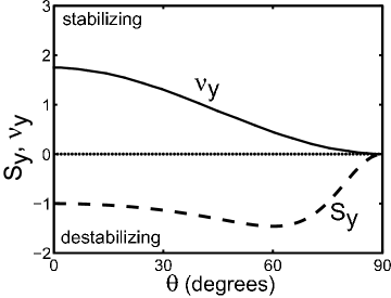
Figure 3: Normalized coefficients $S_{x},\nu_{x},S_{y}$, and $\nu_{y}$, comparing the effect of surface-induced currents ($\nu$, Eq. 27) to erosion from Gaussian ellipsoids ($S$, Eq. 1). The relative magnitude of $\nu/S$ at normal incidence varies with conditions and is chosen arbitrarily here for illustrative purposes.

Notably, the mechanism described by Eq. (27) corresponds to a conserved surface current and thus does not have any effect on the yield curve $I(b)$. The effect of induced surface currents on the stability is evident in Fig. 3. The effect stabilizes both modes from normal incidence up to incidence angles of $45^{o}$, whereupon it becomes a destabilizing influence on only the longitudinal mode. The magnitudes of $\nu_{x}$ and $\nu_{y}$ must equal each other at normal incidence, but their relationship to the magnitudes of $S_{x}$ and $S_{y}$ depends on the relative strengths of the mechanisms. If the induced surface current mechanism is sufficiently strong, as illustrated in Fig. 3, then starting with normal incidence and going to increasing angles, one should observe a regime of absolute stability; the dominance of parallel modes; and the dominance of perpendicular modes. For further insight, it is essential to estimate the strength of the induced surface current and how it depends on materials and ion beam parameters, e.g. by methods such as atomistic simulations.

V Experimental Signatures

We have described several mechanisms by which surface dynamics of the form (1) can account for regions of ion beam angle where a flat surface can be stable or unstable. The mechanisms suggested in the previous two sections provide some scenarios leading to modifications of the Bradley-Harper coefficients in Eq. (1) and thereby causing stability of the bombarded surface at various ranges of angles; there are also potentially other such mechanisms.

The critical question now is to determine which of the potential physical effects is operating in experiments; the answer to this question almost certainly depends on the material, the ion mass and energy, etc. Beyond the linear stability analysis itself, this issue is of central importance for developing a quantitative nonlinear theory of pattern formation; it is well known Cross and Hohenberg (1993) that accurately identifying the linear dispersion relation is critical for deriving a nonlinear theory which can predict the fully developed pattern.

How can experiments discern the dominant linear (in)stability mechanism? Here we present one method for ruling out some of the possibilities: in particular we point out the relevance of the stability-instability transition not only as an interesting dynamical phenomenon, but as a conceptual tool to gain valuable information on the general character of the dynamics of ion sputtered surfaces further away from the transition.

In general, the linear stability analyses discussed in this paper result in a dispersion relation of the form:

$$R_{q}\equiv Re\ (\omega_{\bf q})=-{S_{x}^{eff}}q_{x}^{2}-{S_{y}^{eff}}q_{y}^{2}-B_{xx}q_{x}^{4}-B_{yy}q_{y}^{4}-B_{xy}q_{x}^{2}q_{y}^{2}+\cdots\ ,$$ (31)

Makeev et al. (2002) which describes the growth rate of a Fourier mode:

$$\hat{h}_{q_{x},q_{y}}(t)=\hat{h}_{q_{x},q_{y}}(0)e^{i(q_{x}x+q_{y}y)+\omega_{\bf q}t}\ .$$ (32)

In equation (31) we have lumped the two quadratic contributions into $S_{x,y}^{eff}=S_{x,y}-\nu_{x,y}$. We focus on the transition between stable and unstable perpendicular (parallel) modes described by Eq. (31) as $S_{y}^{eff}$ ($S_{x}^{eff}$) changes sign. This is depicted in the left column of Fig. (4).

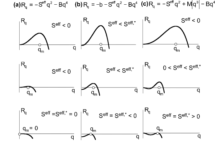
Figure 4: Schematic plots depicting the transition between stable and unstable surface dynamics for three dispersion relations. (a) Left column: generalized Bradley-Harper, Eq. (31), where the transition occurs at $S^{\rm{eff,*}}=0$ with diverging wavelength. (b) Middle column: with Facsko nonlocal “damping term”, transition occurs at $S^{\rm{eff,*}}<0$ with finite wavelength. (c) Right column: with Asaro-Tiller nonlocal elastic energy mechanism, transition occurs at $S^{\rm{eff,*}}>0$ with finite wavelength.

Here we assume for simplicity that the only parameters in Eq. (31) that change appreciably with the beam angle are $S_{x}^{eff},S_{y}^{eff}$.

The most important feature of this schematic plot is that it predicts divergence of the pattern wavelength upon reaching the transition to stable surface dynamics. To see this more clearly, notice that a condition for the existence of linearly unstable modes is that $\max(R_{q})$, the maximal value of $R_{q}$ over all wave vectors ${\bf q}=(q_{x},q_{y})$ is positive. Assuming a smooth dependence of all coefficients on the beam angle, a transition between stable and unstable surface dynamics corresponds to a beam angle for which $\max(R_{q})=0$. For simplicity, let us assume that $\max(R_{q})$ is achieved for ${\bf q}=(q_{max},0)$. Then: $q_{max}=\sqrt{-S_{x}^{eff}/2B_{xx}}$ and $\max(R_{q})=R_{(q_{max},0)}=-S_{x}^{eff}/4B_{xx}=0$, implying $S_{x}^{eff}(\theta)\to S^{*}=0$ and hence $q_{max}\to 0$ at the transition.

A diverging length scale is a strong characteristic signature of the stability-instability transition, and it is thus natural to ask whether this prediction is valid if other physical processes, not accounted for in this paper, influence the surface dynamics and thus modify the dispersion relation (31). We argue that this divergence is expected as long as the following assumptions are satisfied:

1. The beam-angle dependence of all coefficients in the equation is smooth.

2. The linear dynamics is analytic, ruling out terms like $|\nabla h|$

3. The dynamics is first order in time.

4. Linear surface dynamics is local - namely, it can be described by a partial differential equation (PDE).

Assumption 1 is required because, as can be seen easily from Fig. (4a), a discontinuous ”jump” between negative and positive values of $S_{x}^{eff},S_{y}^{eff}$ at some beam angle $\theta^{*}$ may yield a transition to stable dynamics at $|q|>0$. Physically, a discontinuous change of parameters is associated with abrupt changes in material properties, such as amorphization of a crystalline surface. For such a scenario to be associated with a smooth change of the beam angle is sufficiently unlikely as to be a rare occurrence. Assumption 2 is required in order to make a linear stability analysis meaningful. If this assumption is violated then the early stage surface dynamics of an initially flat surface is not described by the dynamics of independently evolving Fourier modes (32). Assumption 3 is expected to hold as long as inertia is neglected. Assumptions 3 and 4 together imply that the the amplification rate $R_{q}$, which is the real part of the complex eigen-frequency $\omega_{q}$, contains only even positive powers of $q$. Namely, local processes, by which a change of surface height is related to the variation of erosion or flux rates between a surface point and its nearest neighbors can be described by spatial derivatives of the function $h(x,y,t)$. In a dynamics that is first order in time, the eigen-frequency $\omega_{q}$ in Eq. (32) thus equals a polynomial in $q$, where all spatial derivatives with odd order (i.e. $\nabla h$, $\nabla^{3}h$) have imaginary coefficients, and thus do not contribute to the amplification rate $R_{q}=Re\ (\omega_{q})$. Notice also that the locality assumption rules out the existence of a constant term (i.e. $\propto q^{0}$) in (32). This is a consequence of the invariance $h\to h+const.$. Therefore, a term $\propto h(x,y,t)$ (i.e. without spatial derivatives) can appear in the surface dynamics only as a combination respecting this invariance such as $h(x,y,t)-\bar{h}(t)$, where $\bar{h}(t)=\int d{\bf x}h({\bf x,t})$, and thus must be associated with some nonlocal processes.

Thus, under these general assumptions (and neglecting the possibility that spatial derivatives of order 6 or higher are dominant in the dynamics), the amplification rate $R_{q}$ satisfies Eq. (31), the stability-instability transition is depicted by Fig. (4a), and the characteristic wavelength at the transition is predicted to diverge.

Recently, Ziberi Ziberi (2006) and George George (2007) have measured the pattern wavelength at several values of beam angles near the transition to the stable region in silicon irradiated by noble gas ions at temperatures where the surface should be amorphous and isotropic. The measurements indicate that the wavelength at the transition remains finite, and may thus be a strong indication that one of the above assumptions is violated. Anticipating that assumptions 1-3 are still valid, we will discuss here two nonlocal terms, whose introduction may render the wavelength at the transition finite.

V.1 Facsko “damping” term

First, let us consider the effect of including a linear term, $\bar{K}[h(x,y,t)-\bar{h}(t)]$ with $\bar{h}(t)=\int d{\bf x}h({\bf x,t})$, in the surface dynamics, Eq. (1). Such a term was recently introduced by Facsko et. al. Facsko et al. (2004) as a possible way to obtain long range ordered patterns observed in the fully nonlinear regime. The term is suggested to be a placeholder for a model of redeposition. With such a term, a constant $\bar{K}$ is added to the right hand side of the dispersion relation (31). This is consistent with the dispersion relation measured by Brown and Erlebacher Brown and Erlebacher (2005) on Si(111) at temperatures where it should remain crystalline, with singular surface energetics (making the validity of assumption (2) questionable). The effect of this term on the transition between stable and unstable dynamics is depicted in the middle column of Fig. (4), where it is demonstrated that the characteristic wavelength does not diverge at the transition, as can be obtained from the following analysis: Again, for simplicity we assume that $\max(R_{q})$ is achieved for ${\bf q}=(q_{max},0)$. Here again $q_{max}=\sqrt{-S_{x}^{eff}/2B_{xx}}$ but $\max(R_{q})=R_{(q_{max},0)}=K-S_{x}^{eff}/4B_{xx}=0$, implying $S_{x}^{eff}(\theta)=S^{*}<0$ and hence $|q_{max}|>0$ at the transition.

V.2 Asaro-Tiller mechanism

The Asaro-Tiller elastic energy driven mechanism Asaro and Tiller (1972); Grinfeld (1086) gives rise to instability of solid surfaces under biaxial in-plane stress. Biaxial compressive stresses are known to develop in the bombarded solidBrongersma et al. (2002); Hedler et al. (2005); van Dillen et al. (2005); Otani et al. (2006); Kim et al. (2006); Meek et al. (1971); van Dillen et al. (2003), and this effect could be important in the surface dynamics. Assuming a sinusoidal modulation of a free surface under biaxial compressive stress, the tangential stress increases at the troughs (compression) and decreases at the peaks (dilation) by an amount proportional to the wavenumber of the modulation and to the applied stress $\sigma_{0}$ in the solid. This increases the chemical potential at the troughs compared to the peaks and drives a surface current from the troughs to the peaks that further amplifies the modulation, thus leading to instability. Including this effect in the surface dynamics gives rise to a term $\propto M|q|^{3}$ on the RHS of Eq. (31) Panat et al. (2005), where $M\propto\sigma_{0}^{2}$. This term does not stem from local effects but rather from nonlocal effects associated with reducing elastic energy throughout the whole solid. The effect of such a term on the transition from stable to unstable surface dynamics is depicted in the right-hand column of Fig. 4. As usual, we simplify the analysis by assuming that $\max(R_{q})$ is achieved for ${\bf q}=(q_{max},0)$ and solve the two equations: (i) $R_{q}=0$ and (ii) $\partial R_{q}/\partial q=0$, from which we get $S_{x}^{eff}(\theta)=S^{*}=M^{2}/4B_{xx}>0$ and $|q_{max}|=M/2B_{xx}>0$ at the transition.

In this analysis we have implicitly assumed that the transition from stable to unstable dynamics is “supercritical” - namely, that it is triggered by infinitesimal perturbations, and thus associated with a change of sign of $\max(R_{q})$. It is also possible that the transition is “subcritical”, and occurs at parameters for which the linear stability analysis, Eq. (31) yields $\max(R_{q})<0$. If the transition is subcritical, then the characteristic wavelength may not diverge even if the linear dispersion is of the form (31). It is possible to discern supercritical from subcritical transitions by probing signatures of hysteretic behavior (associated with subcritical but not with supercritical transitions), and by carefully analyzing the kinetics of pattern formation. A necessary condition for the existence of a subcritical transition is that the leading nonlinear contributions to the dynamics have a destabilizing effect (unlike the stabilizing nonlinear terms derived in Makeev et al. (2002)). Because our analysis is restricted to the linear dynamics we will not pursue this possibility further here.

VI Conclusions

While the possibility of producing patterned surfaces has attracted significant attention recently, few experiments have focused on regions in parameter space where dynamically stable, smooth surfaces are observed. The existence of these stable regions contradicts the Bradley-Harper stability analysis, but this is only part of the reason for their importance: we have argued in this paper that the emergence of stable surfaces provides important insights into the surface dynamics, that are critical for the development of a nonlinear theory of pattern formation in any parameters regime of ion sputtering. Our major messages are:

1. The Bradley-Harper prediction regarding the instability of ion-bombarded surfaces to perpendicular mode ripples follows from a broad class of purely erosive response functions. This robustness may explain why the Bradley-Harper picture seems to describe correctly many observations of pattern evolution on ion sputtered surfaces.

2. Various types of non-erosive response can change the sign of the coefficient of the second spatial derivative and thereby change the stability of surfaces to the emergence of large scale patterns. In particular, modifications of the response can lead to linear stability of smooth surfaces at various ranges of beam angles. These changes can be accompanied by no observable modification of the yield curve. Evidence for such modifications should thus come from atomistic simulations or from experiments that are capable of probing the local surface response to a single ion impact.

3. Careful analysis of qualitative features of the pattern near the transition between stability and instability of a flat surface, in particular the existence or lack of divergence of the pattern wavelength at the transition, enable us to determine conclusively whether nonlocal mechanisms significantly affect the surface dynamics. The outcome of this analysis is extremely important: because the existence of nonlocal terms qualitatively changes the linear dispersion relation, they must be included in the surface dynamics, even away from the transition regime.

This paper focused on the linear dynamics of ion sputtered surfaces. In order to predict and control the fully developed patterns it is necessary to extend this to a nonlinear analysis. The existence of a stable-unstable transition at a critical beam angle $\theta_{c}$ presents an excellent opportunity for quantitative predictions about pattern formation. Typically, near such a transition only a few Fourier modes are unstable, and the morphology of evolving patterns can generally be described by a weakly nonlinear “amplitude equation”, whose form is universal and is determined almost solely by symmetry considerations Cross and Hohenberg (1993). In other contexts, such amplitude equations have been enormously successful at predicting the shape of the selected patterns and many more features of their dynamics. Such an approach has not been tried so far for ion sputtered surfaces, apparently because it has been assumed that there is no continuous control parameter whose variation may change the stability of flat surfaces. Recognizing that the beam angle is exactly such a parameter, at least for certain surfaces and ion types and energies, may enable the application of this invaluable theoretical tool to quantitative study of pattern formation on ion sputtered surfaces.

We hope that the theoretical directions outlined in this paper will trigger experimental and computational work that will lead to better understanding of the surface response to ion impact and its relevance to large scale surface dynamics, and to better characterization of the transition from stability to instability of flat surfaces. We believe that such insights will be important to the development of a quantitative theory that will predict whether and what types of patterns are formed on a sputtered surface for a given set of material and ion beam parameters.

Acknowledgements The research of BD was supported through the Harvard MRSEC; the research of MJA was supported through DE-FG02-06ER46335, and the research of MPB was supported through NSF-0605031. BD acknowledges NWO for a travel grant and the hospitality of the Lorentz Institute at Leiden University, where part of this work was done. We thank W. Van Saarloos for pointing our attention to the importance of careful analysis of the stable-unstable transition. We thank H. Bola George for helpful discussions and for preparing the plots in Fig. 4. We thank N. Kalyanasundaram, H.T. Johnson and J.B. Freund for helpful discussions.

References

- Navez et al. (1962) M. Navez, D. Chaperot, and C. Sella, Comptes Rendus Hebdomadaires Des Seances De L Academie Des Sciences 254, 240 (1962).
- Carter et al. (1977) G. Carter, M. Nobes, F. Paton, J. Williams, and J. Whitton, Rad. Eff. 33, 65 (1977).
- Lewis et al. (1980) G. Lewis, M. Nobes, G. Carter, and J. Whitton, Nuc. Inst. and Meth. 170 (1980).
- Bradley and Harper (1988) R. M. Bradley and J. M. E. Harper, J. Vac. Sci. Technol. A 6, 2390 (1988).
- Malherbe (1994) J. Malherbe, Critical Reviews in Solid State and Materials Sciences 19, 129 (1994).
- Mayer et al. (1994) M. Mayer, E. Chason, and A. Howard, J. Appl. Phys. 76, 1633 (1994).
- Chason et al. (1994) E. Chason, T. Mayer, B. Kellerman, D. McIlroy, and A. Howard, Phys. Rev. Lett. 72, 3040 (1994).
- Cuerno and Barabasi (1995) R. Cuerno and A.-L. Barabasi, Phys. Rev. Lett. 74, 4746 (1995).
- Carter and Vishnyakov (1996) G. Carter and V. Vishnyakov, Phys. Rev. B 54, 17647 (1996).
- Makeev and Barabasi (1997) M. Makeev and A.-L. Barabasi, Appl. Phys. Lett. 71, 2800 (1997).
- Facsko et al. (1999) S. Facsko, T. Dekorsy, C. Koerdt, C. Trappe, H. Kurz, A. Vogt, and H. Hartnagel, Science 285, 1551 (1999).
- Judy et al. (1999) A. Judy, M. R. Murty, E. Butler, J. Pomeroy, B. Cooper, A. Woll, J. Brock, S. Kycia, and R. Headrick, Mater. Res. Soc. Symp. Proc. 570, 61 (1999).
- Erlebacher et al. (1999) J. Erlebacher, M. J. Aziz, E. Chason, M. B. Sinclair, and J. Floro, Phys. Rev. Lett. 82, 2330 (1999).
- Erlebacher et al. (2000) J. Erlebacher, M. J. Aziz, E. Chason, M. B. Sinclair, and J. A. Floro, J. Vac. Sci. Technol. A 18, 115 (2000).
- Facsko et al. (2001) S. Facsko, T. Bobek, T. Dekorsy, and H. Kurz, Phys. Stat. Sol. B 224, 537 (2001).
- Flamm et al. (2001) D. Flamm, F. Frost, and D. Hirsch, Appl. Surf. Sci. 179, 95 (2001).
- Habenicht (2001) S. Habenicht, Phys. Rev. B 63, 125419 (2001).
- Costantini et al. (2001) G. Costantini, F. B. de Mongeot, C. Boragno, and U. Valbusa, Phys. Rev. Lett. 86, 838 (2001).
- Umbach et al. (2001) C. Umbach, R. Headrick, and K. Chang, Phys. Rev. Lett. 87, 246104 (2001).
- Valbusa et al. (2002) U. Valbusa, C. Boragno, and F. B. de Mongeot, J. Phys.: Condens. Matter 14, 8153 (2002).
- Makeev et al. (2002) M. A. Makeev, R. Cuerno, and A.-L. Barabasi, Nucl. Instr. and Meth. in Phys. Res. B 197, 185 (2002).
- Chason and Aziz (2003) E. Chason and M.J. Aziz, Scripta Mater. 49, 953 (2003).
- Facsko et al. (2004) S. Facsko, T. Bobek, A. Stahl, H. Kurz, and T. Dekorsy, Physical Review B 69 (2004).
- Castro et al. (2005) M. Castro, R. Cuerno, L. Vazquez, and R. Gago, Phys. Rev. Lett. 94, 016102 (2005).
- Chan and Chason (2005) W. Chan and E. Chason, Phys. Rev. B 72, 165418 (2005).
- Cuenat et al. (2005) A. Cuenat, H. B. George, K.-C. Chang, J. Blakely, and M. J. Aziz, Adv. Mater. 17, 2845 (2005).
- Feix et al. (2005) M. Feix, A. Hartmann, R. Kree, J. Munoz-Garcia, and R. Cuerno, Phys. Rev. B 71 (2005).
- Rusponi et al. (1997) S. Rusponi, C. Boragno, and U. Valbusa, Phys. Rev. Lett. 78 (1997).
- Brown and Erlebacher (2005) A. Brown and J. Erlebacher, Phys. Rev. B 72, 075350 (2005).
- Brown et al. (2005) A. Brown, J. Erlebacher, W. Chan, and E. Chason, Phys. Rev. Lett. 95, 056101 (2005).
- Ziberi et al. (2005) B. Ziberi, F. Frost, T. Hoche, and B. Rauschenbach, Phys. Rev. B 72, 235310 (2005).
- Ziberi et al. (2006) B. Ziberi, F. Frost, and B. Rauschenbach, J.Vac. Sci. Technol. A 24, 1344 (2006).
- Aziz (2006) M. J. Aziz, Mat. Fys. Medd. Dan. Vid. Selsk. 52 187 (2006).
- Sigmund (1969) P. Sigmund, Phys. Rev. 184, 383 (1969).
- Sigmund (1973) P. Sigmund, J. Mater. Sci. 8, 1545 (1973).
- Herring (1950) C. Herring, J. Appl. Phys. 21, 301 (1950).
- Mullins (1959) W. Mullins, J. Appl. Phys. 30, 77 (1959).
- Cross and Hohenberg (1993) M. Cross and P. Hohenberg, Rev. Mod. Phys. 65 (1993).
- Yamada et al. (2001) I. Yamada, J. Matsuo, N. Toyoda, and A. Kirkpatrick, Mater. Sci. Eng. R-Reports 34, 231 (2001).
- Bringa et al. (2001) E. Bringa, K. Nordlund, and J. Keinonen, Phys. Rev. B 64, 235426 (2001).
- Kalyanasundaram et al. (2007) N. Kalyanasundaram, H. Johnson, and J. Freund, unpublished.
- Moseler et al. (2005) M. Moseler, P. Gumbsch, C. Casiraghi, A. Ferrari, and J. Robertson, Science 309, 1545 (2005).
- Vasile et al. (1999) M. Vasile, J. Xie, and R. Nassar, J. Vac. Sci. Technol. B 17, 3085 (1999).
- Ziberi (2006) B. Ziberi Ph.D. Thesis, University of Leipzig (2006).
- George (2007) H. George, Ph.D. Thesis, Harvard University (2007).
- Asaro and Tiller (1972) R. Asaro and W. Tiller, Metall. Trans. 3, 1789 (1972).
- Grinfeld (1086) M. Grinfeld, Sov. Phys. Dokl. 31, 831 (1086).
- Brongersma et al. (2002) M. Brongersma, E. Snoeks, T. van Dillen, and A. Polman, J. Appl. Phys. 88 (2002).
- Hedler et al. (2005) A. Hedler, S. Klaumunzer, and W. Wesch, Phys. Rev. B 72 (2005).
- van Dillen et al. (2005) T. van Dillen, A. Polman, P. Onck, and E. van der Giessen, Phys. Rev. B 71, 024103 (2005).
- Otani et al. (2006) K. Otani, X. Chen, J. Hutchinson, J. Chervinsky, and M.J. Aziz, J. Appl. Phys. 100, 023535 (2006).
- Kim et al. (2006) Y.-R. Kim, P. Chen, M.J. Aziz, D. Branton, and J.J. Vlassak, J. Appl. Phys. 100 (2006).
- Meek et al. (1971) R. Meek, W. Gibson, and J. Sellscho, Applied Physics Letters 18, 535 (1971).
- van Dillen et al. (2003) T. van Dillen, A. Polman, and C. M. van Kats, Applied Physics Letters 83, 4315 (2003).
- Panat et al. (2005) R. Panat, K. Hsia, and D. Cahill, J. Appl. Phys. 97 (2005).
- Villain (1991) J. Villain, Journal De Physique I 1, 19 (1991).