Monte Carlo Simulations of an Extended Feynman-Kikuchi Model

Abstract

We present Quantum Monte Carlo simulations of a generalization of the Feynman-Kikuchi model which includes the possibility of vacancies and interactions between the particles undergoing exchange. By measuring the winding number (superfluid density) and density structure factor, we determine the phase diagram, and show that it exhibits regions which possess both superfluid and charge ordering.

I Introduction

The study of continuum superfluid phase transitions using Quantum Monte Carlo (QMC) methods has a history which includes path integral simulations of Helium using realistic interatomic potentials, which capture $T_{\lambda}$ in good quantitative agreement with experiment ceperley82 , to recent numerical work newcontinuumsupersims focusing on experiments chan05 ; moreexpts which observe ‘supersolid’ order supersolidreviews , the simultaneous presence of both superfluidity and long range density correlations.

At the same time, related path integral studies of lattice models (the ‘boson-Hubbard’ Hamiltonian) fisher89 ; jaksch98 have been undertaken. These too have been partially motivated by the issue of supersolid order, but have also been driven by the possibility of studying the universal conductivity in granular superconductors univcond , and superfluid-Mott insulator transitions of relevance to optically trapped atoms jaksch98

Many of these simulations emphasize Feynman’s picture of the connection between the superfluid transition and the increasing entanglement (and ultimate development of macroscopic ‘winding’ across the whole sample) of quantum paths as the temperature is lowered. Indeed, the superfluid density $\rho_{s}$ is proportional to the mean square winding of paths around the latticeceperley82 .

However, even before the advent of these large scale QMC simulations which allow the study of the superfluid transition exactly, Feynmanfeynman53 and Kikuchikikuchi54 ; kikuchi60 suggested, and studied analytically, an approximate ‘classical’ model whose configurations are permutation loops of sites on a $d=3$ lattice. The partition function they suggested is,

$$Z=\int\prod_{i=1}^{N}d{\bf r}_{i}\sum_{\cal P}\rho({\bf r}_{1},{\bf r}_{2},\cdots,{\bf r}_{N})$$

$$\times\,\,{\rm exp}\,\big{[}\,\,-{m_{\rm eff}k_{\rm B}T\over 2\hbar^{2}}\sum_{i}({\bf r}_{i}-{\cal P}{\bf r}_{i})^{2}\,\,\big{]}\,\,.$$ (1)

Here $m_{\rm eff}$ is the effective mass of He atoms, and the function $\rho({\bf r}_{1},{\bf r}_{2},\cdots,{\bf r}_{N})$ is assumed to be nonvanishing only when the coordinates ${\bf r}_{i}$ are located on the sites of a regular lattice (a cubic lattice in the original treatments). ${\cal P}$ refers to a permutation of the coordinates. A transition to a ‘superfluid’ phase where a macroscopic number of sites participate in a single large loop, as the temperature $T$ is lowered, was discovered and investigated.

Various approximations were employed to determine the properties of this model, predominantly diagrammatic (series) expansions in the exchange loops. To faclitate these analytic treatments, in many of the early studies the allowed permutations were restricted to “near-neighbor” exchange in which the maximum “distance traveled” by each particle $i$, is only one lattice constant $d$. That is, $|{\bf r}_{i}-{\cal P}{\bf r}_{i}|=d$ for all particles $i$. One of the early issues concerned whether the superfluid transition was third order, as originally found by Feynman feynman53 , or second order chester54 ; rice54 ; matsubara54 ; terhaar54 and whether the order was affected by the restriction to near-neighbor exchange. Another issue was the behavior of the specific heat, both how to eliminate various artificial structures (and even negative values) near the phase transition, and also how to recover the experimentally observed $T^{3}$ behavior in superfluids at low temperatures. Here the removal of the restriction to local permutations was found to be crucial kikuchi60 .

The Feynman-Kikuchi (FK) model is closely related to the duality-transformed $XY$ model dasgupta81 ; elser84 , where the partition function can also be expressed in terms of sums of closed paths on a lattice. The allowed configurations are somewhat different, since in the $XY$ case path overlap is allowed whereas in the FK model, each ${\bf r}_{i}$ appears only once in ${\cal P}{\bf r}_{i}$. However, the energy for paths grows quadratically with the overlap, so that in practice large overlaps are unlikely, enhancing the similarities between the partition functions. This connection is perhaps not so surprising since both models offer ways to understand the superfluid phase transition.

In this paper we will study the FK model in $d=2$ using Monte Carlo simulations elser84 . Motivated by recent work on supersolids, we will then suggest a generalization which contains ‘vacancies’ and interactions between the occupied sites. We will determine the nature of the superfluid phase transition, and how it depends on particle density, and also study the possibility of charge ordered states arising from the interactions. The results allow up to construct the phase diagram of our generalized FK model.

II Model and Computational Methods

We begin by briefly reviewing the motivation for the FK model which will expose the connection with exact path integral expressions for the partition function. Consider the quantum Hamiltonian for a system of $N$ interacting bosons,

$$\hat{H}=\sum_{i=1}^{N}{\hat{\bf p}_{i}^{2}\over 2m}+V(\hat{\bf r}_{1},\hat{\bf r}_{2},\cdots\hat{\bf r}_{N})\,\,.$$ (2)

Here $\hat{\bf p}_{i}$ and $\hat{\bf r}_{i}$ are the momentum and position operators. The partition function is given by,

$$Z = {\rm Tr}\,e^{-\hat{H}/T}={\rm Tr}\,\big{[}\,e^{-\epsilon\hat{H}/T}\cdots\,e^{-\epsilon\hat{H}/T}\,\big{]}$$ (3)

$$\approx {\rm Tr}\,\big{[}e^{-\epsilon\hat{K}/T}\,e^{-\epsilon\hat{V}/T}\cdots\,e^{-\epsilon\hat{K}/T}\,e^{-\epsilon\hat{V}/T}\,\big{]}$$

where, following the usual the path integral approach feynman65 ; creutz81 , a small parameter $\epsilon$ has introduced, the exponential of the full Hamiltonian has been broken into $M$ pieces with $M\epsilon=1$, and then approximated by the product of the exponentials of the kinetic and potential energies individually. This ‘Trotter’ approximationtrotter ; suzuki ; fye becomes exact in the limit $\epsilon\rightarrow 0$ ($M\rightarrow\infty$). We have set Boltzmann’s constant $k_{\rm B}=1$ for simplicity.

The trace is evaluated by summing over a complete set of position eigenstates, and also inserting additional complete sets of position eigenstates throughout the string of incremental imaginary time evolution operators. The potential energy exponentials act on the eigenstates to give numbers, and the remaining matrix elements of the kinetic energy operators are readily computed, yielding,

$$Z = \sum_{\cal P}\,\int\prod_{i=1}^{N}\prod_{m=1}^{M}d{\bf r}_{i}^{m}\,e^{-S}$$

$$S = {\epsilon\over T}\sum_{m=1}^{M}V({\bf r}_{1}^{m},{\bf r}_{2}^{m},\cdots{\bf r}_{N}^{m})$$ (4)

$$+ {\epsilon\over T}\sum_{m=1}^{M}\sum_{i=1}^{N}\big{[}{{\bf r}_{i}^{m+1}-{\bf r}_{i}^{m}\over\epsilon/T}\big{]}^{2}\,\,.$$

Here the superscript $m$ is an ‘imaginary time’ index which labels the point of insertion of the different complete sets of states. The final set of positions $\{{\bf r}_{i}^{M}\}$ is constrained to be a permutation ${\cal P}$ of the original positions $\{{\bf r}_{i}^{1}\}$, as a consequence of the trace in the definition of the quantum partition function. The sum over permutations ${\cal P}$ incorporates the indistiguishability of the bosonic particles. This completes the representation of the partition function as an integral over classical paths in space and imaginary time.

Examination of this exact expression for the partition function, now readily motivates the origin of the FK model. The function $\rho({\bf r}_{1},{\bf r}_{2},\cdots,{\bf r}_{N})$, and its restriction to a cubic lattice, can be thought of as arising from the potential energy terms which act to tend to localize the particle positions in a regular array. The single exponential in the particle positions in the FK model can be regarded as a truncation of the complete set of $M$ exponentials for all imaginary times. Notice that the combination of the leading factor $\epsilon/T$ and the two such factors in the denominator of the ‘kinetic energy’ lead to the appearance of the temperature in the numerator. From the viewpoint of the original path integral, this reflects the fact that as the temperature is lowered, the paths have more (imaginary) time in which to propagate, and it becomes increasingly easy for them to permute. Physically, this then leads to a superfluid phase transition as $T$ is lowered.

In this paper, we will work with the FK model on a two dimensional square lattice. We will denote by $\beta$ the inverse of the prefactor of the sum of the distances traveled by the individual particles. That is, our partition function will be,

$$Z=\sum_{{\cal P}}{\rm exp}\big{[}-{E\over\beta}\big{]}=\sum_{{\cal P}}{\rm exp}\,\big{[}-{1\over\beta}\sum_{i}({\bf r}_{i}-{\cal P}{\bf r}_{i})^{2}\big{]}$$ (5)

To be explicit, to a labeling of the sites of the two dimensional square lattice, illustrated in Fig. 1 (left) we associate a permutation ${\cal P}$. An example is shown in Fig. 1 (right). This configuration contains three nontrivial permutation loops: The particles at sites 8 and 9 are in a ‘two particle’ loop, as are the particles at sites 5 and 18. Note that in the former each particle moves a single lattice site, and contributes ‘1’ to the energy, while the square of the distances traveled by each particle in the latter case is 5. The fourth and fifth rows contain a loop of five particles (moving distances $({\bf r}_{i}-{\cal P}{\bf r}_{i})^{2}=5,1,2,1,$ and $1$) which extends (‘winds’) all the way across the lattice in the $x$ direction. The remaining sites, which share the same labels in the left and right, correspond physically to particles which have not undergone an exchange. The total energy $E$ of the three loops in this configuration ${\cal P}{\bf r}_{i}$ is $E=(1+1)+(5+5)+(5+1+2+1+1)=22$.

The periodic boundary conditions produce an ambiguity in the definition of the energy, since there is more than one way in which to compute the distance traveled by each particle. We define the energy by choosing the smallest of such distances.

In order to monitor the superfluid phase transition we measure the winding across the lattice in the $x$ and $y$ directions. $W_{x}$ counts the difference between the number of particles which move to the right across the vertical edge of the lattice and those which move to the left. An analogous definition applies for $W_{y}$ across the top, horizontal edge. We define $W^{2}=W_{x}^{2}+W_{y}^{2}$. In the right panel of Fig. 1, $W_{x}=1$ and $W_{y}=0$.

Figure 1: Left: Unpermuted labeling of the sites in a $6\times 6$ lattice. Right: Representative configuration in our simulation. The energy $E=22$ and the windings $W_{x}=1,W_{y}=0$. See text for explanation.

We now introduce our extension of the FK model to allow for vacancies. In so doing, we are motivated by recent work on ‘supersolid’ phases chan05 ; newcontinuumsupersims which are, in fact, continuations of an extensive history. In the configuration in the right panel of Fig. 1, each site is labeled by one of the 36 sites in the left panel. All sites are occupied. We can define a set of ‘vacancies’ by assigning ‘0’ to a subset of the sites in the lattice (Fig. 2, left). An allowed configuration ${\cal P}({\bf r}_{i})$ of the system has zeroes at the same sites as the vacant sites in ${\bf r}_{i}$ and the occupied site labels are permuted. An example is given in Fig. 2 (right). By a similar calculation to that described for Fig. 1, the configuration shown has energy $E=20$. Note that we will consider “annealed” vacancies: the vacancy density is fixed, but the system is allowed to sample all possible density locations satisfying that global constraint.

Figure 2: Left: Unpermuted labeling of the sites in a $6\times 6$ lattice when the number of bosons $N_{b}=31<36$. Empty sites are labeled by zeroes. Right: Representative configuration in our simulation of our extension of the FK model. See text for explanation.

Once vacancies are allowed, it is possible to introduce additional terms in the summand of the partition function which control their relative positions on the lattice. We choose to add the simplest possible term,

$$E_{v} = +V\sum_{\langle ij\rangle}(\,1-\delta_{0,{\cal P}{\bf r}_{i}}\,)\,(\,1-\delta_{0,{\cal P}{\bf r}_{j}}\,)$$ (6)

$$= +V\sum_{\langle ij\rangle}(\,1-\delta_{0,{\bf r}_{i}}\,)\,(\,1-\delta_{0,{\bf r}_{j}}\,)\,\,\,.$$

The sum is over neighboring sites $\langle ij\rangle$ of the lattice. $E_{v}$ adds $V$ to the energy for each link which connects sites both of which are occupied. As emphasized in Eq. 6, this number is the same whether the permuted or unpermuted sites are used in the summand, since the collection of occupied sites before and after the exchanges is the same.

The resulting partition function combines the original FK exchange term and the new interaction term,

$$Z = \sum_{{\cal P}}{\rm exp}\,\big{[}\,\,-{1\over\beta}\sum_{i}({\bf r}_{i}-{\cal P}{\bf r}_{i})^{2}\,\,$$ (7)

$$- \beta\,V\sum_{\langle ij\rangle}(\,1-\delta_{0,{\cal P}{\bf r}_{i}}\,)\,(\,1-\delta_{0,{\cal P}{\bf r}_{j}}\,)\big{]}\,\,.$$

The inverse temperature $\beta$ appears in the interaction term in its usual place.

We conclude this section by briefly discussing our simulation algorithm. Our approach is a straightforward implementation of the Metropolis Monte Carlo method binder80 . We suggest a change in our permutation which consists of interchanging two, randomly selected, entries ${\cal P}{\bf r}_{i}$ and ${\cal P}{\bf r}_{j}$ in the permutation ${\cal P}$. If a vacancy is moved, the list of occupied sites and their permutation must be changed accordingly. The resulting change $\Delta$ in the argument of the exponential appearing in the partition function is evaluated, and the change is accepted with probability $p={\rm min}\,(\,1,e^{-\Delta}\,)$.

As with most path integral simulations, such local moves have difficulty evolving the configuration through phase space at large $\beta$ where the important paths are dominated by large loops. We therefore also introduce ‘global’ moves which shift the elements ${\cal P}{\bf r}_{i}$ by one lattice constant for sites $i$ across an entire column or row of the lattice. Such moves change the vertical or horizontal winding of the lattice by $\Delta W=\pm 1$. In some simulations such moves have low acceptance rates as the system size increases. Indeed, this is a primary limitation of simulations of real Helium ceperley82 . However, we do not encounter this difficulty here.

III Simulation Results: Feynman-Kikuchi Model

We begin by studying the original FK model. In Fig. 3 we show data for the mean square winding $\langle W^{2}\rangle$ as a function of $\beta$ for different lattice sizes. We see that the winding becomes nonzero as $\beta$ increases, and that the onset of nonzero winding becomes increasingly sharp as the lattice size grows. This raw data is suggestive of a critical $\beta_{c}\approx 0.6$ for the development of macroscopic loops. In simulations of the FK model in which only local exchanges are allowed, on a $d=3$ cubic lattice elser84 , Elser finds $\beta_{c}\approx 0.69$. Presumably the higher dimensionality lowers $\beta_{c}$ relative to our $d=2$ square lattice while the restriction to local exchage would tend to raise $\beta_{c}$. Hence a rough match of the critical points is plausible.

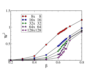
Figure 3: Raw data for the mean square winding as a function of $\beta$ on lattice sizes ranging from $8\times 8$ to $128\times 128$.

We can make the case for a phase transition, and determine $\beta_{c}$ with higher precision, by scaling our raw data. We adopt the usual ansatz cardy88 which postulates that the dependence of the order parameter on the parameter controlling the transition and on the lattice size takes the scaling form,

$$W^{2}\,(L,\beta)=L^{a}f\big{[}\,L^{b}(\beta-\beta_{c})\,\big{]}\,\,.$$ (8)

Here $f$ is a universal (lattice size independent) function of its argument, and $a$ and $b$ are critical exponents.

This scaling form is usefully rewritten as,

$$L^{-a}W^{2}\,(L,\beta)=f\big{[}\,L^{b}(\beta-\beta_{c})\,\big{]}\,\,.$$ (9)

From this expression it is clear that if we scale the order parameter $\langle W^{2}\rangle$ by the lattice size to an appropriate exponent, $L^{-a}\langle W^{2}\rangle$, and plot as a function of the control parameter $\beta$, all the curves will cross at the universal value $f(0)$ when $\beta=\beta_{c}$, regardless of the value of the second exponent $b$.

Fig. 4 presents the results of the analysis in which the vertical (order parameter, $\langle W^{2}\rangle$) axis alone is scaled. We observe a universal crossing of the five curves, and infer $\beta_{c}=0.62\pm 0.01$ and $a=0.61\pm 0.03$.

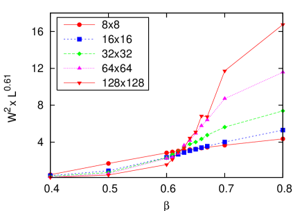
Figure 4: Raw data of Fig. 3 for the mean square winding scaled by the lattice size. The intersection of the curves determines $\beta_{c}=0.62\pm 0.01$.

We calculate the average energy and specific heat from the partition function using the standard thermodynamics formulae,

$$<E>=-\frac{\partial\ln Z}{\partial\beta}\hskip 36.135ptC=\frac{\partial E}{\partial T}$$ (10)

Fig. 5 shows a plot of specific heat as a function of temperature. We used the temperature rather than $\beta$ as our horizontal axis, as is more conventional. We see that there is a peak in the specific heat at roughly the same position as the crossing of the winding $T_{c}=1/\beta_{c}=1/0.62=1.61$.

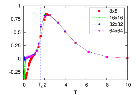
Figure 5: Plot of specific heat for the original FK model, that is, a fully filled lattice with no vacancies and no interactions. The value of the critical temperature inferred from the scaling of the winding (Fig. 4) is indicated as a vertical dotted line. The negative values of $C(T)$ at low $T$ are a finite size artifact, as explained in the text.

The specific heat exhibits a sharp drop, and goes negative, close to $T=0$. This is a non-physical effect which appears due to the finite size of the lattice, as can be seen as follows. Starting with the partition function of Eq. 5 we obtain,

$$E=-\frac{\partial\ln Z}{\partial\beta}=-\frac{1}{\beta^{2}}\frac{\mathop{\sum}_{n}Ke^{-\frac{K}{\beta}}}{Z_{0}}=-\frac{1}{\beta^{2}}\;\langle E\rangle$$ (11)

where $Z_{0}=\mathop{\sum}_{n}e^{-\frac{K}{\beta}}$ is the partition function used in Monte Carlo simulations; $\langle E\rangle$ is our MC calculation of energy. The specific heat

$$C = \frac{\partial E}{\partial T}=\frac{\partial E}{\partial(1/\beta)}$$ (12)

$$= -\frac{1}{\beta}\langle E\rangle+\frac{1}{\beta^{2}}\left(\langle E^{2}\rangle-{\langle E\rangle}^{2}\right)$$

$$= -\frac{1}{\beta}B+\frac{1}{\beta^{2}}A$$

For a finite lattice, as $\beta\rightarrow\infty$, $A$ and $B$ approach constant values given by all permutations on the $L\times L$ lattice having equal probability. As a consequence, as $\beta\rightarrow\infty$,

$$-\frac{1}{\beta}B+\frac{1}{\beta^{2}}A=\frac{1}{\beta^{2}}(A-B\beta)\;\rightarrow 0^{-}$$

So at large $\beta$, or small $T$, the specific heat becomes negative, achieves its minimum, and goes back to zero, as $T\rightarrow 0$. As the lattice size increases, the area of negative specific heat moves closer to $T=0$. This is because the situation when all permutations have approximately equal probability occurs when $K/\beta\rightarrow 0$, or $L^{2}/\beta\rightarrow 0$, so $\beta\sim L^{2}$, or $T\sim L^{-2}$ for this area of negative specific heat.

Despite the crudity of the model, we can, following Feynman and Kikuchifeynman53 ; kikuchi54 , use these results to infer a rough critical temperature for Helium, The scaling of the winding gives $\beta_{c}=0.62$, or $T_{c}=1.62$. To recover physical values for the temperature we note our unit is $T_{1}=\hbar^{2}/k_{B}md^{2}$, where $m$ is the mass of boson, and $d$ is lattice spacing. For ⁴He, using density of 146 $kg/m^{3}$, and $d=3.57\cdot 10^{-10}m$, we obtain $T_{1}=0.95K$. This puts our transition temperature around 1.5 K, which is in the same ballpark as $T_{\lambda}$ for Helium.

We close this section by examining the low $T$ behavior of the specific heat, since obtaining the proper exponent was the focus of much of the original work on the FK model. In three dimensions, where the initial analytic studies were performed, a linearly dispersing (phonon) mode $E(k)=ck$ gives $C(T)\;\sim\;T^{3}$ at low $T$. Here we are working in $d=2$, where instead $C(T)\;\sim\;T^{2}$. Fig. 6 shows an attempt to fit $C(T)$ to a power law. The least squares fit gives $C(T)\;\sim\;T^{1.95\pm 0.1}$ for lattices of different sizes, which is in reasonable agreement with the prediction based on a linearly dispersing mode. (We restrict our fit to temperatures higher than those at which the finite size artifact negative $C(T)$ values onset.)

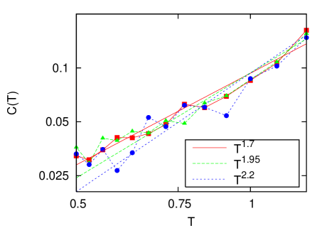
Figure 6: A log-log plot of specific heat versus temperature yields data consistent with a straight line of slope $1.95\pm 0.1$, in agreement with the expected value, 2. We used a temperature range $0.5\leq T\leq 1.25$, where $T$ is small, but out of range of the (non-physical) dip in $C$,

IV Simulation Results: Extended Feynman Kikuchi Model

We now turn to our generalization of the FK model in which we allow a lattice with partial filling and a repulsive interaction $V$ between nearest neighbor sites. We study first the special case of half-filling, where it is possible to have perfect ordering of the vacancies/particles in a “checkerboard” pattern.

IV.1 Half-filling: $\langle\rho\rangle\;=\;\frac{1}{2}$

How does the introduction of vacancies affect $\beta_{c}^{\,{\rm sf}}$ in the absence of interactions, $V=0$? (Henceforth in this manuscript we will append a superscipt ‘sf’ to $\beta_{c}$ for the superfluid transition, to distinguish it from the $\beta_{c}^{\,{\rm cdw}}$ for charge ordering. See below.) Figs. 7 and 8 are the analogues of Figs. 3 and 4, and show the unscaled and scaled winding as a function of $\beta$. As before, we have done simulations for lattices of different sizes to perform the finite size scaling. The crossing occurs at $\beta_{c}^{\,{\rm sf}}=1.50\pm 0.02$. By repeating this sweep of $\beta$ for different $V$, we can compute the superfluid phase boundary $\beta_{c}^{\,{\rm sf}}(V)$ in the $V-\beta$ plane at half-filling. This is shown in Fig. 11.

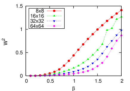
Figure 7: Raw data for $\langle W^{2}\rangle$ for the extended FK model with half-filling and $V=0$.

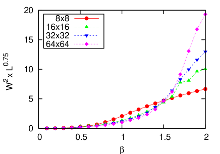
Figure 8: Data of Fig. 7, scaled. We infer $\beta_{c}^{\,{\rm sf}}=1.50\pm 0.02$.

A natural question to ask is whether $E_{v}$ induces vacancy/density ordering. We define the real space density correlation function,

$$c({\bf r},{\bf r}\,^{\prime})\;=\;\langle\,\,\left(\rho({\bf r})-\left<\rho\right>\right)\left(\rho({\bf r}\,^{\prime})-\left<\rho\right>\right)\,\,\rangle\,\,\,,$$ (13)

where the density $\rho({\bf r}_{i})=1$ if the site $i$ is occupied and is zero otherwise. The structure function,

$$S({\bf q})=\;\frac{1}{N^{2}}\mathop{\sum}_{{\bf r},{\bf r}\,^{\prime}}e^{i{\bf q}\cdot({\bf r}-{\bf r}\,^{\prime})}c({\bf r},{\bf r}\,^{\prime})\,\,\,,$$ (14)

is the Fourier transform of the density correlations. Here $N$ is number of sites. At half-filling, the ordering vector ${\bf q}=(\pi,\pi)$. In a disordered phase where $c({\bf r},{\bf r}\,^{\prime})$ decays exponentially with $|{\bf r}-{\bf r}^{\prime}|$, $S({\bf q})$ will vanish in the thermodynamic limit (proportional to $1/N$). In an ordered phase, $S({\bf q)}$ will go to a constant as the system size increases, for the appropriate ordering wave vector ${\bf q}$.

Proceeding in analogy with the winding $\langle W^{2}\rangle$, we measure $S(\pi,\pi)$ for different lattice sizes and do finite size scaling to determine $\beta_{c}^{\,{\rm cdw}}$ for the CDW transition. Representative plots, for $V=2.5$, are shown in Figs. 9 and 10. Putting together such sweeps for different interaction strengths $V$ yields the density order-disorder (CDW) phase boundary in the $\beta-V$ plane at half-filling shown in Fig. 11.

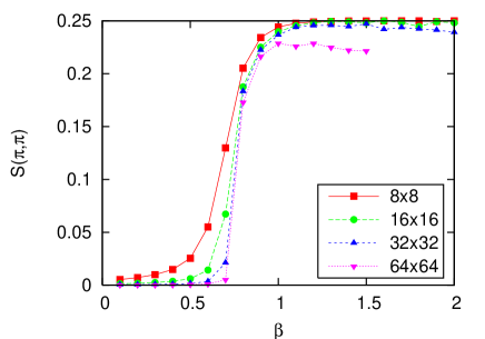
Figure 9: The structure factor $S(\pi,\pi)$ is shown as a function of $\beta$ at half-filling and $V=2.5$.

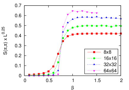
Figure 10: Scaled data of Fig. 9. The crossing point defines $\beta_{c}^{\,{\rm cdw}}$ for CDW ordering. The scaling exponent multiplying $S$ on the vertical axis is that of the $d=2$ Ising model, as discussed in the text.

In fact, a number of aspects of the phase diagram of Fig. 11 can be inferred by a mapping to the Ising model. We note that the interaction energy $E_{v}$ of Eq. 6 maps precisely to that of the Ising model (the well-known equivalence of lattice-gas and Ising models) with the definition of the spin $S^{z}_{i}=2(\rho({\bf r}_{i})-\frac{1}{2})$. The alternating occupied and empty site pattern caused by the repulsive particle-particle interaction ($V>0$) corresponds to an antiferromagnetic arrangement in spin language. The quantity $V/4$ plays the role of the exchange constant $J$. The critical temperature of the Ising model given by the Onsager solution $T_{c}=2.269J$ then implies a density ordering $\beta_{c}^{\,{\rm cdw}}=4/(2.269\,V)=1.763/V$. We expect this result to be accurate for $V>>\beta$ where $E_{v}$ dominates over any effects on the site densities which might be caused by the exchange term. This curve is shown as the dotted line in Fig. 11.

We can also make a qualitative argument for how the phase boundary might bend away from this Ising limit as the role of $\beta$ becomes larger. For any given density arrangement, the exchange of particles provides additional configurations of the system associated with permutations of the particle indices. Such configurations have lower energy when the occupied sites are adjacent. Thus we expect that the exchange term will favor “ferromagnetic” spin configurations, in competition with the “antiferromagnetism” driven by $E_{v}$. This suggests a lowering of the CDW transition temperature. Just such an increase in $\beta_{c}^{\,{\rm cdw}}$ is seen in the phase diagram. One may well ask whether there is an extreme limit where the attraction between particles due to the greater ease of exchange becomes so dominant that phase separation occurs (ferromagnetic clusters in spin language). We will address this possibililty later.

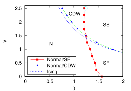
Figure 11: The central result of our paper: Phase diagram of the extended Feynman-Kikuchi model in the $V-\beta$ plane at half-filling. Squares denote simulation results for the superfluid transition, and triangles the CDW transition. The CDW boundary is in good correspondence with the Ising limit $\beta_{c}^{\,{\rm cdw}}=4/(2.269\,V)$, indicated by the dotted line. The circle at $V=2.5$ is the prediction $\beta_{c}^{{\,\rm sf}}(\rho)=\beta_{c}^{\,{\rm sf}}(\rho=1)/\rho$. See text for details.

The corresponding effect of $V$ on the superfluid phase transition is less easy to describe rigorously, in part because we do not begin from a known limit like the Onsager solution in the density transition case. On the one hand, increasing $V$ drives the particles apart, making local exchange more expensive, suggesting that $\beta_{c}^{\,{\rm sf}}$ might increase. On the other hand, the superfluid transition is not caused by local exchange but instead by global winding, and by separating the particles, $V$ might help provide regularly spaced “stepping stones,” aiding global winding and decreasing $\beta_{c}^{\,{\rm sf}}$. While these qualitative arguments provide different conclusions, numerically, the answer is clear from Fig. 11: turning on $V$ decreases $\beta_{c}^{\,{\rm sf}}$. The effect is not large, however.

In the limit of large $V$ and half-filling, a perfect CDW phase forms, which corresponds to a completely filled square lattice with a lattice constant $\sqrt{2}$ larger than the original lattice (and rotated by 45 degrees). The squared distances in the FK exchange energy will be scaled up by a factor of two, and hence $\beta_{c}^{\,{\rm sf}}$ will be twice the value for the no-vacancy FK model of the previous section. Thus $\beta_{c}^{\,{\rm sf}}=2\,(0.62\pm 0.01)$. This value is shown as the circle at $V=2.5$ in Fig. 11.

In order to develop a simple understanding of $\beta_{c}^{\,{\rm sf}}$ for general $V$, we consider a small (four site, two particle) cluster and enumerate completely the allowed configurations. There are six possible density configurations, which separate into two classes. Four of them have the two particles adjacent, while the other two have the two particles separated by vacancies:

$$\begin{array}[]{l@{\;\;\;|\;} l@{\;\;\;|\;} l@{\;\;\;|\;} l@{\;\;\;|\;}}{\rm Configuration}&{\rm K\;energy}&{\rm P\;energy}&{\rm Weight}\\ \hline\cr\bullet-\bullet-\circ-\circ&1/2+9/2&V&4\,e^{-\left(\frac{5}{\beta}+V\beta\right)}\\ \hline\cr\bullet-\circ-\bullet-\circ&4/2+4/2&0&2\,e^{-\left(\frac{4}{\beta}\right)}\\ \end{array}$$ (18)

We have included the degeneracy factors in the weight. For each density configuration, there are two permutations. Since we are interested in the superfluid transition, we will restrict ourselves to the case where the two particles do exchange, which is reflected in the nonzero value of the kinetic energy in the table above.

The expectation value of the Kinetic energy is

$$\langle K\rangle = \frac{2\cdot 5e^{-\left(\frac{5}{\beta}+V\beta\right)}+4e^{-\left(\frac{4}{\beta}\right)}}{2e^{-\left(\frac{5}{\beta}+V\beta\right)}+e^{-\left(\frac{4}{\beta}\right)}}$$ (19)

$$= 4+\frac{2}{2+e^{\left(\frac{1}{\beta}+V\beta\right)}}$$

Note that $\langle K\rangle=4$ is kinetic energy at $V\rightarrow\infty$. The superfluid transition occurs when $K\sim\beta$. If we set $\langle K\rangle=\beta_{c}^{\,{\rm sf}}$ and use $\langle K(V\rightarrow\infty)\rangle=4=\beta_{c}^{\,{\rm sf}}(V\rightarrow\infty)$ we find that the shift in the superfluid transition is given by,

$$\frac{\Delta\beta_{c}}{\beta_{c}(V\rightarrow\infty)}=\frac{1}{2}\cdot\frac{1}{2+e^{\left(\frac{1}{\beta}+V\beta\right)}}$$ (20)

This result is qualitatively correct at $V=0$, predicting a small positive shift in $\beta_{c}^{\,{\rm sf}}$ relative to $V\rightarrow\infty)$.

IV.2 Doped system $\langle\rho\rangle\;\neq\;\frac{1}{2}$

In this section we consider general filling $\rho$. Specifically, in Fig. 12 we exhibit the phase diagram in the $\beta-\rho$ plane for two fixed values of the interaction, $V=1.25$ and $V=2.50$. Fig. 12 was obtained using the same analysis as in the earlier sections: Evaluation and scaling of the winding and structure factor as a function of $\beta$ for different $V$ and $\rho$. Several features are immediately apparent from the phase diagram: Charge ordering is, as expected, favored close to half-filling, with the highest transition temperature at $\rho=1/2$. Interestingly, the shape and size of the density ordered region around half-filling is in rough agreement with the boundaries obtained for checkerboard solid order in the extended boson-Hubbard model batrouni00 ; hebert02 where similar superfluid and charge ordered phases are present in an explicitly quantum model.

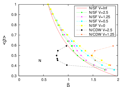
Figure 12: Phase diagram in the $\rho-\beta$ plane for the extended FK model for different values of $V$. Triangles: the numerically obtained cdw transitions. Squares: the numerically obtained superfluid transitions. The superfluid phase boundary is reasonably well approximated by $\beta_{c}^{\,{\rm sf}}\propto 1/\rho$ (solid curve). See text.

In the preceding section we argued that $\beta_{c}^{\,{\rm sf}}$ for half-filling and $V=\infty$ should be a factor of two larger than for the original, no vacancy FK model, and showed this was borne out numerically. One might expect that a similar result would be true for general fillings and that $\beta_{c}^{\,{\rm sf}}$ would be increased by a factor of $1/\rho$, since this factor reflects the increase in the square of the average interparticle spacing.

$$\beta_{c}^{\,{\rm sf}}(\rho,V\rightarrow\infty)=\frac{1}{\rho}\beta_{c}^{\,{\rm sf}}(\rho=1)$$ (21)

However, on further consideration, it is not quite so. Half-filling and $V=\infty$ is a special case and in general the particles are not dispersed uniformly, that is, they no longer all have the same distance from their nearest neighbors. Nevertheless, this relation provides a reasonable guide to the density dependence of the superfluid transition, and is shown on phase diagram at Fig. 12 as the line “$N/SF\;V={\rm Inf}$”. In Fig. 12 we also see that as $\beta$ is increased at $\rho=1/2$ and fixed $V=1.25$, we go from normal to superfluid to supersolid, where the phases are labeled by the behavior of the two order parameters, $\langle W^{2}\rangle$ and $S(\pi,\pi)$. Likewise at larger $V=2.50$ we go from normal to CDW to supersolid.

While the order parameters provide unambiguous identification of the phases, it is also interesting to see if the thermodynamics can pick up the two successive transitions in the form of separate peaks in the specific heat. To study $C(T)$, we proceed similarly to the derivation for the partition function with only the kinetic energy term. Now our partition function has both potential and kinetic energy.

$$Z = \mathop{\sum}_{n}e^{-P\beta-\frac{K}{\beta}}$$

$$E = -\frac{\partial\ln Z}{\partial\beta}=\frac{\mathop{\sum}_{n}\left(P-\frac{K}{\beta^{2}}\right)e^{-P\beta-\frac{K}{\beta}}}{Z_{0}}$$

$$C = \frac{\partial E}{\partial T}=\frac{\partial E}{\partial(1/\beta)}$$ (22)

$$= -\left(\langle P\rangle\beta-\frac{\langle K\rangle}{\beta}\right)^{2}$$

$$+ \left\langle\left(P\beta-\frac{K}{\beta}\right)^{2}\right\rangle-\frac{\langle K\rangle}{\beta}$$

Fig. 13 shows the specific heat as a function of temperature for half-filling and interaction $V=1.25$. According to the phase diagram Fig. 12, the two transition points are $N/SF$ at $\beta=1.26$ ($T=0.79$) and $N/CDW$ at $\beta=1.47$ ($T=0.68$). As can be seen, we cannot resolve separate peaks in $C(T)$ associated with these transitions. It is likely that the critical temperatures are too close and that the finite size rounding blurs the two peaks into a single maximum.

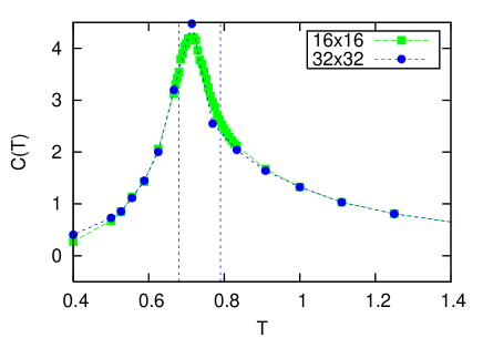
Figure 13: Specific heat for half-filling, $V=1.25$. From Fig. 12, the $SF$ transition is at $T=0.79$, and the $CDW$ transition at $T=0.68$. These values are shown as vertical dashed lines. The specific heat cannot resolve the two peaks.

We can however exhibit separate SF and CDW peaks in the specific heat if we push the transitions apart sufficiently. For example, at $V=10$ the CDW transition occurs at a much higher temperature than the SF transition. Indeed, in Fig. 14 we can now observe separate signatures of the two transitions in $C(T)$. The maxima occur close to the transition points given by the order parameters.

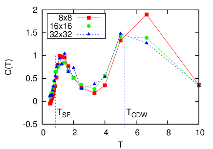
Figure 14: Specific heat for half-filling and $V=10$. Two peaks corresponding to SF and CDW transitions are clearly seen. The critical values given by the winding and structure factor are shown as vertical dashed lines. The Ising mapping would give $T_{CDW}=5.67$.

Our final results concern the possibility of phase separation. One might argue that in a model with vacancies, especially at low or vanishing $V$, the particles will clump together in order to facilitate exchange. Indeed, phase separation has been observed in a related model: the bose Hubbard Hamiltonian with ring exchange, precisely due to this mechanism rousseau04 .

Phase separation is signalled by a peak in the density structure factor at small momenta ${\bf q}$ (as opposed to the CDW ordering vector at the largest ${\bf q}=(\pi,\pi)$). Crudely speaking there are real space density fluctuations at long wavelengths, corresponding to a lattice with one side half occupied and the other half empty. These translate into a peak in $S({\bf q})$ at small ${\bf q}$. Note that in a canonical ensemble simulation such as is performed here we cannot set ${\bf q}=(0,0)$ since that value of the structure factor is just a constant set by the filling. Indeed with our definition of the density correlations in terms of fluctuations about the average density per site, Eq. 14, $S(0,0)=0$.

For a perfectly phase separated state with all particles on the right-most half of the lattice we find $S(2\pi/L,0)\approx 0.11$ for $L=16$. In Fig. 15 we see that $S(2\pi/L,0)$ is $\sim\;1/100$ of that figure for $V>0$. We conclude there is no phase separation in this model. The absence of a signal for phase separation is in contrast to the behavior in the related bose-Hubbard model with ring exchange rousseau04 ; rousseau05 There the same quantity, the average of the structure factors at the three lowest momenta shows a sharp rise with increased exchange, as one enters the superfluid phase.

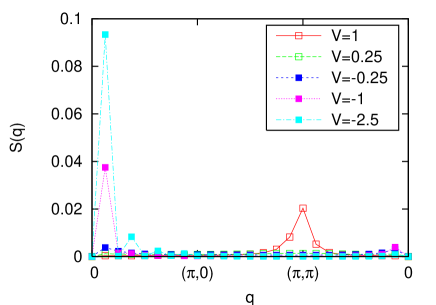
Figure 15: $S(\vec{q})$ for various $V$, $L=16$, $\beta=1.5$. $S(2\pi/L,0)$ should signal phase separation if it is $\sim\;0.1$. It is however not close to that number for $V>0$. For comparison, plots for $V<0$ are given, and they indicate phase separation.

Conclusions

In this paper we have presented Monte Carlo simulations of the phase diagram of an extension of the $d=2$ Feynman-Kikuchi model which includes vacancies. We found phases which have density and superfluid order, and where these two types of order coexist. Unlike the boson-Hubbard model where supersolid order requires doping away from half-filling in the extended FK model $\rho_{s}$ is nonzero even in the defect-free checkerboard solid. The reason is that the boson-Hubbard kinetic energy moves particles only between near-neighbor sites. Bosons cannot exchange without passing through an energetically unfavorable region. But in the FK model, exchange at longer range can occur without ever ‘passing through’ the rare configurations with near-neighbor sites that are occupied. One might expect that in the FK model which is restricted to local exchange, the half-filled supersolid might be eliminated.

A further problem of interest in the extended FK is to consider “quenched” vacancies in which the locations of the empty sites are frozen throughout the simulation. Here again we might expect that when a restriction to local exchange is enforced, there could be a destruction of the superfluid transition as the percolation threshold is crossed. In the model allowing exchanges of arbitrary distance, one expects a more trivial increase in $\beta_{c}$, but that the superfluid transition would likely persist.

A final avenue for exploration would be the inclusion of a one-body vacancy potential which could be chosen to confine the particles preferentially towards the center of the lattice. Such simulations would connect with recent experiments on cold atoms in magnetic and laser traps.

We acknowledge support from the National Science Foundation under award NSF ITR 0313390, and useful input from T.Tremeloes.

References

- (1) D.M. Ceperley, Phys. Rev. B30, 2555 (1984); D.M. Ceperley and E.L. Pollock, Phys. Rev. Lett. 56, 351 (1986); and E.L. Pollock and D.M. Ceperley, Phys. Rev. B36, 8343 (1987).
- (2) D. M. Ceperley and B. Bernu Phys. Rev. Lett. 93, 155303 (2004); M. Boninsegni, A. B. Kuklov, L. Pollet, N. V. Prokof’ev, B. V. Svistunov, and M. Troyer, Phys. Rev. Lett. 97, 080401 (2006); Bryan K. Clark and D. M. Ceperley, Phys. Rev. Lett. 96, 105302 (2006).
- (3) E. Kim and M. H. Chan, Science 305, 1941 (2004).
- (4) James Day, Tobias Herman, and John Beamish, Phys. Rev. Lett. 95, 035301 (2005); E. Kim and M. H. Chan, Phys. Rev. Lett. 97, 115302 (2006); I. A. Todoshchenko, H. Alles, J. Bueno, H. J. Junes, A. Ya. Parshin, and V. Tsepelin, Phys. Rev. Lett. 97, 165302 (2006); Ann Sophie Rittner and John D. Reppy, Phys. Rev. Lett. 97, 165301 (2006); M. A. Adams, J. Mayers, O. Kirichek, and R. B. Down, Phys. Rev. Lett. 98, 085301 (2007); Ann Sophie Rittner and John D. Reppy, Phys. Rev. Lett. 98, 175302 (2007).
- (5) G. Chester, Phys. Rev. A2, 256 (1970); A.F. Andreev, “Quantum Crystals,” in Progress in Low Temperature Physics, Vol. VIII, D.G. Brewer (Ed.), North Holland, Amsterdam, (1982); and A.J. Leggett, Phys. Rev. Lett. 25, 1543 (1970).
- (6) M.P.A. Fisher, P.B. Weichman, G. Grinstein and D.S. Fisher, Phys. Rev. B40, 546 (1989).
- (7) D. Jaksch, C. Bruder, J.I. Cirac, C.W. Gardiner, and P. Zoller, Phys. Rev. Lett. 81, 3108 (1998).
- (8) M. Cha, M.P.A. Fisher, S.M. Girvin, M. Wallin, and A.P. Young, Phys. Rev. B44, 6883 (1991); E.S. Sorensen, M. Wallin, S.M. Girvin, and A.P. Young, Phys. Rev. Lett. 69, 828 (1992); G.G. Batrouni, B. Larson, R.T. Scalettar, J. Tobochnik, and J. Wang, Phys. Rev. B48, 9628 (1993); and K.J. Runge, Phys. Rev. B45, 13136 (1992).
- (9) R.P. Feynman, Phys. Rev. 90, 1116 (1953); Phys. Rev. 91, 1291 (1953); Phys. Rev. 91, 1301 (1953); Phys. Rev. 94, 262 (1954).
- (10) R. Kikuchi, Phys. Rev. 96, 563 (1954).
- (11) R. Kikuchi, H. Denman, and C.L. Schreiber, Phys. Rev. 119, 1823 (1960).
- (12) G.V. Chester, Phys. Rev. 93, 1412 (1954).
- (13) O.K. Rice, Phys. Rev. 93, 1161 (1954).
- (14) T. Matsubara, Busseiron Kenkyu 72, 78 (1954).
- (15) D. ter Haar, Phys. Rev. 95, 895 (1954).
- (16) C. Dasgupta and B.I. Halperin, Phys. Rev. Lett. 47, 1556 (1981).
- (17) As far as we know, the only Monte Carlo simulations of the Feynman Kikuchi model are contained in V. Elser, Ph.D. thesis, unpublished. These studies are in , and consider a local exchange restricted model.
- (18) Quantum Mechanics and Path Integrals, R.P. Feynman and A.R. Hibbs, McGraw-Hill, New York (1965).
- (19) M. Creutz and J. Freedman, Annals of Phys. 132, 427 (1981).
- (20) H.F. Trotter, Proc. Am. Math. Soc. 10, 545 (1959).
- (21) M. Suzuki, Phys. Lett. 113A, 299 (1985).
- (22) R.M. Fye, Phys. Rev. B33, 6271 (1986); and R.M. Fye and R.T. Scalettar, Phys. Rev. B36, 3833 (1987).
- (23) Monte Carlo Simulation in Statistical Physics, K. Binder and D.W. Heermann, Springer, 1980.
- (24) Finite Size Scaling, J. Cardy, ed. Elsevier, 1988.
- (25) G.G. Batrouni and R.T. Scalettar, Phys. Rev. Lett. 84, 1599 (2000).
- (26) F. Hébert, G.G. Batrouni, R.T. Scalettar, G. Schmid, M. Troyer and A. Dorneich, Phys. Rev. B65 014513 (2002).
- (27) V. Rousseau, G. G. Batrouni, and R.T. Scalettar, Phys. Rev. Lett. 93, 110404 (2004).
- (28) V.G. Rousseau, R.T. Scalettar, and G.G. Batrouni, Phys. Rev. B72, 054524 (2005).
- (29) Andras Suto, J. Phys. A35 6995 (2002).
- (30) Daniel Gandolfo, Jean Ruiz, and Daniel Ueltschi, cond-mat/0703315.