Unzipping Vortices in Type-II Superconductors

Abstract

The unzipping of vortex lines using magnetic-force microscopy from extended defects is studied theoretically. We study both the unzipping isolated vortex from common defects, such as columnar pins and twin-planes, and the unzipping of a vortex from a plane in the presence of other vortices. We show, using analytic and numerical methods, that the universal properties of the unzipping transition of a single vortex depend only on the dimensionality of the defect in the presence and absence of disorder. For the unzipping of a vortex from a plane populated with many vortices is shown to be very sensitive to the properties of the vortices in the two-dimensional plane. In particular such unzipping experiments can be used to measure the “Luttinger liquid parameter” of the vortices in the plane. In addition we suggest a method for measuring the line tension of the vortex directly using the experiments.

I Introduction

The competition between thermal fluctuations, pinning and interactions between vortices leads to many novel physical phenomena in type-II high-temperature superconductors blatter . Examples include the melting of the Abrikosov flux-lattice into an entangled vortex-liquid ns and the proposed existence of low temperature Bose-glass nv , vortex glass fisher_glass and Bragg glass nat_sch phases.

Many experimental probes have been used to study these phenomena. They include decoration, transport and magnetization measurements, neutron scattering, electron microscopy, electron holography and Hall probe microscopes. More recently it has become possible to manipulate single vortices, for example using magnetic force microscopy (MFM) Wadas92 . These can, in principle, measure directly many microscopic properties which have been up to now under debate or assumed. The possibility of performing such experiments is similar in spirit to single molecule experiments on motor proteins, DNA, and RNA which have opened a window on phenomena inaccessible via traditional bulk biochemistry experiments singlemol .

In this spirit Olson-Reichhardt and Hastings ORH04 have proposed using MFM to wind two vortices around each other. Such an experiment allows direct probing of the energetic barrier for two vortices to cut through each other. A high barrier for flux lines crossing has important consequences for the dynamics of the entangled vortex phase.

In this paper we introduce and study several experiments in which a single vortex is depinned from extended defects using, for example, MFM. A brief account of the results can be found in Ref. [knp, ]. First we consider a setup where MFM is used to pull an isolated vortex bound to common extended defects such as a columnar pin, screw dislocation, or a twin plane in the presence of point disorder. Using a scaling argument, supported by numerical and rigorous analytical results, we derive the displacement of the vortex as a function of the force exerted by the tip of a magnetic force microscope. We focus on the behavior near the depinning transition and consider an arbitrary dimension $d$. We argue that the transition can be characterized by a universal critical exponent, which depends only on the dimensionality of the defect. We show that unzipping experiments from a twin plane directly measures the free-energy fluctuations of a vortex in the presence of point disorder in $d=1+1$ dimensions. To the best of our knowledge, there is only one, indirect, measurement of this important quantity in Ref. [Bolle, ]. The form of the phase diagram in the force temperature plane is also analyzed in different dimensions. Related results apply when a tilted magnetic field is used to tear away vortex lines in the presence of point disorder, which was not considered in earlier work on clean systems. hatano . Furthermore, we show that a possible experimental application of the scaling argument is a direct measurement of the vortex line tension in an unzipping experiment. As we will show in this paper, in a system of finite size, the displacement of the flux line at the transition depends only on the critical force exerted on the flux line by the MFM tip, the flux line tension and the sample thickness. Thus unzipping experiments can provide valuable information on the microscopic properties of flux lines.

Next we consider a setup where a single vortex is pulled out of a plane with many vortices. It is known that the large-scale behavior of vortices in a plane is characterized by a single dimensionless number, often referred to as the Luttinger liquid parameter due to an analogy with bosons in $d=1+1$ dimensions. We show that experiments which unzip a single vortex out of the plane can be used to directly probe the Luttinger liquid parameter. We also discuss the effects of disorder both within the defect and in the bulk with the same setup.

II Unzipping a vortex from a defect

II.1 Review of clean case

We begin by considering the unzipping of a vortex from an extended defect in a clean sample. For a columnar defect the system is depicted in Fig. 1. At the top of the sample the MFM applies a constant force ${\bf f}$ which pulls the vortex away from the defect. We assume that at the bottom of the sample the vortex is always bound to the defect at a specific location. This assumption will not influence the results since below the unzipping transition the flux line is unaffected by the boundary conditions at the far end of the sample.

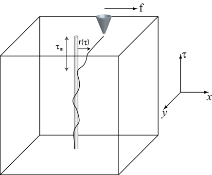
Figure 1: A MFM tip applies a constant force ${\bf f}$ which pulls the vortex away from the defect. The configuration of the vortex is represented by ${\bf r}(\tau)$. We assume throughout that the vortex is always bound to the defect at the bottom of the sample so that ${\bf r}(\tau=0)=0$.

In the absence of external force, and for an external field aligned with the defect, the appropriate energy for a given configuration ${\bf r}(\tau)$ of the vortex is given by blatter :

$$F_{0}\!\!=\!\!\!\int_{0}^{L}\!\!\!\!d\tau\left[\frac{\gamma}{2}(\partial_{\tau}{\bf r}(\tau))^{2}+V({\bf r}(\tau))\right].$$ (1)

Here $\gamma$ is the line tension and $L$ is the length of the sample along the $\tau$ direction. The vector ${\bf r}(\tau)$ represents the configuration of the vortex in the $d$ dimensional space and $V({\bf r})$ is a short-ranged attractive potential describing the $d^{\prime}$-dimensional extended defect (in Fig. 1 $d=3$ and $d^{\prime}=1$). The effect of the the external force, exerted by the MFM, can be incorporated by adding to the free energy the contribution

$$F_{1}=-{\bf f}\cdot{\bf r(L)}=-\int_{0}^{L}{\bf f}\cdot\partial_{\tau}\bf r(\tau)\,d\tau$$ (2)

where we have used ${\bf r}(\tau=0)={\bf 0}$. Here ${\bf f}$ stands for the local force exerted by the MFM in the transverse direction. The free energy of a given configuration of the vortex is given by

$$F({\bf r})=F_{0}({\bf r})+F_{1}({\bf r})\;.$$ (3)

The problem, as stated, has been studied first in the context of vortices in the presence of a tilted magnetic field hatano and the results have been applied to the related problem of DNA unzipping Lubensky .

We note that a similar setup can be achieved by using a transverse magnetic field instead of the external force. See Fig. (2).

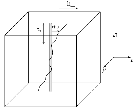
Figure 2: Same as in Fig. 1 but with a transverse magnetic field instead of the MFM force tearing the flux line away from a defect.

Indeed in the free energy (2) the external force couples to the slope of the flux line $\partial_{\tau}{\bf r}$ in the same way as the external magnetic field does hatano . The only difference between the two setups is that there are now equal and opposite forces acting on the top and bottom ends of the sample. However this difference is important only in short samples, where the two ends of the flux line are not independent from each other.

In this paper we focus on the thermal average of distance of the tip of the vortex from the extended defect $\langle x_{m}(\tau=L)\rangle$. This quantity is related to the thermal average of the length of the vortex that is unzipped from the defect, $\langle\tau_{m}\rangle$, through $\langle x_{m}\rangle=f\langle\tau_{m}\rangle/\gamma$. Here and throughout the paper $\langle\ldots\rangle$ denotes a thermal average while an overbar denotes an average over realizations of the disorder.

As stated above the universal behavior of $\langle\tau_{m}\rangle$ (or equivalently $\langle x_{m}\rangle$) within this disorder-free model have been derived previously. Here we sketch two approaches which will be generalized to samples with quenched disorder in the rest of the paper.

In the first approach, instead of directly summing over configurations of the vortex we perform the sum in two parts by dividing the vortex into bound and unbound segments. The unbound segment starts at the point where the vortex departs the defect without ever returning to hit it again up to the top of the sample. Using Eq. (2) it is straightforward to integrate over vortex configurations to obtain for the partition function of the unzipped segment

$$Z_{u}(\tau_{m}) = \int{\cal D}{\bf r}(\tau)\,\mathrm{e}^{-\beta\int_{0}^{\tau_{m}}\!d\tau\left[\frac{\gamma}{2}(\partial_{\tau}{\bf r}(\tau))^{2}-{\bf f}\cdot\partial_{\tau}{\bf r(\tau)}\right]}$$ (4)

$$\propto \mathrm{e}^{\tau_{m}\beta f^{2}/2\gamma}\;,$$

so that the free energy associated with this conditional partition function is

$${\cal F}_{u}(\tau_{m})=-\beta^{-1}\ln Z_{u}(\tau_{m})=-f^{2}\tau_{m}/2\gamma\;,$$ (5)

where $\beta$ is the inverse temperature. Henceforth in this paper we set $\beta=1$, which can be always achieved by appropriate rescaling of the energy units. Even though the above sum also runs over configurations which return to the defect it is easy to verify that these configurations give rise to exponentially small correction in the $\tau_{m}$. Equation (5) implies that as the force, ${\bf f}$, increases the free energy density of the unzipped portion of the vortex decreases. In contrast, the free energy density of the bound part is, clearly, independent of the force and given by ${\cal F}_{b}(\tau_{m})=V_{0}(L-\tau_{m})$, where $V_{0}$ is the free energy per unit length of a bound vortex and $L$ is the length of the sample along the defect. The vortex will be unzipped when $f=f_{c}=\sqrt{2\gamma|V_{0}|}$ such that the free-energy densities of the bound and unzipped states are equal.

In this representation the total free energy of the vortex is given by

$${\cal F}(\tau_{m})={\cal F}_{u}(\tau_{m})+{\cal F}_{b}(\tau_{m})\;.$$ (6)

The unconstrained partition function of the model is given by

$$Z=\int_{0}^{L}d\tau_{m}e^{-(f_{c}^{2}-f^{2})\tau_{m}/2\gamma}\;.$$ (7)

Since both results are independent of the dimensionality of the defect (columnar or planar) near the transition one always finds in the $L\to\infty$ limit

$$\langle\tau_{m}\rangle\sim\frac{1}{(f_{c}-f)^{\nu}}\;,$$ (8)

with $\nu=1$. Note, that it can easily be seen that approaching the transition from above the average length of the vortex which is bound to the defect, $\langle(L-\tau_{m})\rangle$, diverges in the same manner hatano .

An alternative approach, which will also be useful in this paper, uses the mapping of the problem to the physics of a fictitious quantum particle NelsonBook . The contribution of the external field ${\bf f}$ to the free energy now manifests itself as an imaginary vector potential acting on the particle in $d-1$ dimensions (with the $\tau$ axis acting as a time direction). Explicitly, using the standard conversion from path-integrals (see Ref. [hatano, ] for details) one finds that the problem can be described in terms of a non-Hermitian Hamiltonian:

$${\cal H}={1\over 2\gamma}{\bf p}^{2}-{i\over\gamma}{\bf f}\cdot{\bf p}+V({\bf r})\;,$$ (9)

where ${\bf p}=\frac{1}{i}\vec{\nabla}$ is the momentum operator. In this language the vortex is bound to the defect as long as there is a bound state in the Hamiltonian. As mentioned above $i{\bf f}$ is equivalent to a constant imaginary vector potential. This analogy makes it apparent that solutions of the non-Hermitian problem can be related to those of the Hermitian Hamiltonian (where one sets ${\bf f}=0$) by an imaginary gauge-transformation hatano . In particular the left $\psi^{L}_{n}({\bf r},{\bf f})$ and the right $\psi^{R}_{n}({\bf r},{\bf f})$ eigenfunctions of the non-Hermitian problem can be obtained from those of the Hermitian problem, $\psi_{n}({\bf r},{\bf f}={\bf 0})$, using

$$\psi^{R}_{n}({\bf r},{\bf f}) = {\cal U}\psi_{n}({\bf r},{\bf f}={\bf 0})$$

$$\psi^{L}_{n}({\bf r},{\bf f}) = \psi_{n}({\bf r},{\bf f}={\bf 0}){\cal U}^{-1}\;,$$ (10)

where

$${\cal U}=\mathrm{e}^{{\bf f}\cdot{\bf r}}=\mathrm{e}^{fx}\;;\;\;\;\;\;{\cal U}^{-1}=\mathrm{e}^{-{\bf f}\cdot{\bf r}}=\mathrm{e}^{-fx}\;.$$ (11)

The universal behavior of $\tau_{m}$ at the transition, Eq. (8), was obtained in Ref. [hatano, ] by noting that

$$\langle\tau_{m}\rangle\propto\langle x_{m}\rangle={\int x\psi^{R}_{n}({\bf r})d{\bf r}\over\int\psi^{R}_{n}({\bf r})d{\bf r}}\propto{1\over{f_{c}-f}},$$ (12)

where $\psi^{R}_{n}({\bf r})\propto\mathrm{e}^{-f_{c}r}$ at long $r$. We note that the imaginary gauge transformation is justified only at $f<f_{c}$. Otherwise the integrals in Eq. (12) formally diverge. In principle this divergence can be fixed by proper treatment of the boundary conditions AHNS .

Finally we discuss the phase diagram of the model. It is natural that as the temperature rises the value of the critical force needed for the unzipping decreases (at very low temperatures a possible reentrance has been discussed in literature Reentrant ; Reentrant2 ). Here we focus on the existence of a critical force for any strength of the attractive potential. The question is completely equivalent to that of the existence of a localized vortex line in the absence of the external force. Using the analogy to the quantum mechanical problem it is well known that in two dimensions (corresponding to a three dimensional sample) and below, as long as $\int_{-\infty}^{\infty}d{\bf r}V({\bf r})<0$ there exists a bound state. Therefore, in real samples, as long as the potential satisfies this condition there is always a minimum nonzero critical force required to unbind the flux line from the defect.

II.2 Scaling arguments for the disordered case.

II.2.1 Critical Behavior

We now consider the effect of point disorder. In this case the free energy of a given vortex configuration without the contribution from the force exerted by the MFM is given by

$$F_{0}\!\!=\!\!\!\int_{0}^{L}\!\!\!\!d\tau\left[\frac{\gamma}{2}(\partial_{\tau}{\bf r}(\tau))^{2}+V({\bf r}(\tau))+\mu({\bf r}(\tau),\tau)\right].$$ (13)

The frozen point disorder $\mu({\bf r},\tau)$ is assumed to be uncorrelated and Gaussian distributed with $\overline{\mu}=0$ and $\overline{\mu({\bf r},\tau)\mu({\bf r^{\prime}},\tau^{\prime})}=\sigma\delta({\bf r}-{\bf r^{\prime}})\delta(\tau-\tau^{\prime})$. As mentioned above the overbar denotes an average over realizations of the disorder and the $\langle\dots\rangle$ denotes averaging over thermal fluctuations. The contribution from the force exerted by the MFM retains the same form as in Eq. (2).

The free energy, Eq. (13), without the contribution from the external force has been studied previously with and without the presence of an extended defect. Without the defect it is well known that if one fixes one end of the vortex at the bottom of the sample the mean-square displacement, $\langle x^{2}(\tau)\rangle$ of the vortex after traveling a distance $\tau$ into the sample behaves as $\langle x^{2}(\tau)\rangle=B\tau^{2\zeta(d)}$, where $\zeta(d=2)=2/3$ and $\zeta(d=3)\approx 0.61$ is the wandering exponent Karreview . Moreover, for a given realization of disorder there is typically a single dominant trajectory of the vortex and realizations with two competing minima are very rare. Finally, it is known that the free energy fluctuations scale as

$$\delta{\cal F}\propto\tau^{\omega(d)}$$ (14)

with $\omega(d=2)=1/3$, $\omega(d=3)\approx 0.22$. The exponents $\omega$ and $\zeta$ are not independent. They satisfy the scaling relation: $\omega=2\zeta-1$. Note that as long as there is no defect the free energy fluctuations are unaltered even in the presence of a force acting on the vortex because this force can be simply gauged away.

The universal properties of the unzipping transition with point disorder can be analyzed using a simple scaling argument adapted from [Lubensky, ] for the unzipping of DNA (for an abbreviated account, see Ref. [knp, ]).

Following the discussion in the previous section, which analyzed the unzipping problem with no disorder, we sum over configurations of the unzipped part of the vortex and the zipped part of the vortex separately. As before we denote the free energy of the unzipped segment by ${\cal F}_{u}$ and the free energy of the bound segment by ${\cal F}_{b}$. The total free energy is then given by

$${\cal F}(\tau_{m})={\cal F}_{u}(\tau_{m})+{\cal F}_{b}(L-\tau_{m}).$$ (15)

For large $L$ and $\tau_{m}$ we can rewrite

$$\mathcal{F}_{b}(L-\tau_{m})=\mathcal{F}_{b}(L)-\mathcal{F}_{b}(\tau_{m}).$$ (16)

For a one dimensional defect, like a columnar pin, $\mathcal{F}_{b}(L)$ is a constant equal to the free energy of a flux line completely localized on the pin. For higher dimensional defects like a twin plane, there is a subtlety. To see this, consider a zero temperature case first. Then the partition function is determined by the optimal trajectory of a flux line (in the presence of point disorder) starting at $\tau=0$ and ending at $\tau=L-\tau_{m}$. However, this trajectory might not be a part of the optimal trajectory going all the way from $\tau=0$ to $\tau=L$. In this case clearly the relation (16) does not hold. Since this relation does not hold at zero temperature, it should not hold at finite temperatures as well. However, in Ref. [fisher, ] it was argued that such situations (where the optimal trajectories do not coincide) are very rare and can be neglected footnote . Thus ignoring the constant term $\mathcal{F}_{b}(L)$ we can rewrite Eq. (15) as

$${\cal F}(\tau_{m})={\cal F}_{u}(\tau_{m})-\mathcal{F}_{b}(\tau_{m}).$$ (17)

We can identify three contributions to the free energy above. The first is due to the average free energy difference between a vortex on the defect and in the bulk of the sample. Close to the transition, similarly to the analysis in the clean case, it is linear in $\tau_{m}$ and behaves as $a(f_{c}-f)\tau_{m}$, where $a\approx f_{c}/\gamma$ is a positive constant. The second contribution $\delta{\cal F}_{b}$, comes from the free-energy fluctuations arising from that part of the point disorder which is localized on or near the defect. For a columnar defect of dimensionality $d^{\prime}=1$ this contribution is due to the sum of the fluctuations in the free energy about the mean. The central limit theorem implies that it behaves as $\tau_{m}^{1/2}$ at large $\tau_{m}$. For $d^{\prime}>1$ this result is modified and one can use known results for the free energy of a direct path in a random media (see Eq. (14)), which leads to $\delta{\cal F}_{b}\propto\tau_{m}^{\omega(d^{\prime})}$, where $d^{\prime}$ is the dimensionality of the defect Karreview . Finally, there is a contribution to the free energy fluctuations from the interaction of the unzipped part of the vortex with the bulk point disorder, $\delta{\cal F}_{u}$. This contribution behaves similarly to $\delta\mathcal{F}_{b}$ with a different bulk exponent: $\delta{\cal F}_{u}\propto\tau_{m}^{\omega(d)}$, where $d>d^{\prime}$ is the dimensionality of the sample. Collecting all three terms gives:

$${\cal F}(\tau_{m})=a(f_{c}-f)\tau_{m}+\delta\mathcal{F}_{b}(\tau_{m})+\delta\mathcal{F}_{u}(\tau_{m})\;.$$ (18)

As discussed above, $\omega(d)$ has been studied extensively in the past and it is well known that $\omega(d^{\prime})>\omega(d)$ for any $d^{\prime}<d$ Karreview . Therefore, disorder on or close to the defect controls the unbinding transition for any dimension when $\tau_{m}$ is large and the problem is equivalent to unzipping from a sample with point disorder localized on the defect. In particular, this result implies that unzipping from a columnar defect with point disorder in the bulk is in the same universality class as unzipping of a DNA molecule with a random sequence of base pairing energies. In fact, point disorder is likely to be concentrated within real twin planes and near columnar damage tracks created by heavy ion irradiation and near screw dislocations, strengthening even more the conclusions of this simple argument.

The disorder averaged partition function is dominated by the minimum of the free energy and thus by configurations with $\delta\mathcal{F}_{b}(\tau_{m})<0$. Using ${\cal F}(\tau_{m})\approx a(f_{c}-f)\tau_{m}-bm^{\omega(d^{\prime})}$, where $b$ is a positive constant, the partition function

$$Z=\int_{0}^{L}d\tau_{m}e^{-{\cal F}(\tau_{m})}$$ (19)

can be evaluated using a saddle-point approximation. We then find the value of $\tau_{m}$ at the saddle point satisfies $a(f_{c}-f)=\omega(d^{\prime})b\tau_{m}^{\omega(d^{\prime})-1}$. Therefore

$$\overline{\langle\tau_{m}\rangle}\sim\frac{1}{(f_{c}-f)^{\nu}},\;\;\nu=[1-\omega(d^{\prime})]^{-1}\;,$$ (20)

with

$$\nu = 2\;\;\;\;\;\;\;\,{\rm for}\;\;\;d^{\prime}=1$$

$$\nu = 3/2\;\;\;\;{\rm for}\;\;\;d^{\prime}=2\;.$$ (21)

The result for the columnar defect ($d^{\prime}=1$) agrees with known results from DNA unzipping Lubensky .

To check the scaling argument we have preformed numerical simulations in $d=1+1$ dimensions and have been able to solve analytically the closely related problem of vortex unzipping from a wall in $d=1+1$ dimensions. We have also studied the simplified problems of unzipping from a $d^{\prime}=1$ and $d^{\prime}=2$ dimensional defect with disorder localized on the defect. While the $d^{\prime}=1$ problem was solved previously oper ; Lubensky below (in Sec. II.3) we describe a new method applying the replica method. Using some approximations,this approach can be generalized to a $d^{\prime}=2$ dimensional defect. In the next sections we describe all these results which support the simple scaling argument presented above.

II.2.2 Finite size scaling and determination of the flux line tension.

Another consequence of the result (20) is the possibility to perform a finite size scaling analysis privman . In particular, near the unzipping transition the unzipping length $\overline{\langle\tau_{m}\rangle}$ should be a function of the reduced force $\epsilon\propto(f_{c}-f)$ and the system size $L$. If the scaling ansatz (20) is correct then we must have

$$\overline{\langle\tau_{m}\rangle}/L=g(\epsilon L^{1/\nu}),$$ (22)

where $g(x)$ is some scaling function. Quite generally we expect that when $x\gg 1$ finite size effects are unimportant and $g(x)\sim 1/x^{\nu}$ so that we recover the scaling (20) and at $x\ll 1$ we have $g(x)\to g_{0}$, where $g_{0}$ is a constant. Note that the constant $g_{0}$ does not depend on the system size. This constant is a universal number of the order of one, which depends on the dimensionality of the defect. As we find below for the unzipping from a columnar pin $g_{0}=0.5$ and for the unzipping from a twin plane $g_{0}\approx 0.7$. Relation (22) can be used to extract the line tension $\gamma$ through:

$$\gamma=f_{c}g_{0}{L\over\langle x_{m}\rangle}.$$ (23)

Here $f_{c}$ is the critical force and $\langle x_{m}\rangle$ is the displacement of the MFM tip at the transition. To derive Eq. (23) we used the fact that for the unbound segment $\langle x_{m}\rangle=\overline{\langle\tau_{m}\rangle}f/\gamma$.

We emphasize that the unzipping transition is first order both in the clean and disordered cases. Indeed, the unzipping occurs only at the boundary and does not affect total free energy of the flux line in the thermodynamic limit. Nevertheless, similar to wetting phenomena near first order transitions, this transition possesses scaling properties characteristic of second order transitions like diverging correlation lengths, finite size scaling etc.

II.2.3 Phase diagram

Next, we use scaling arguments to consider the behavior of the critical force as the strength of the disorder is varied. In particular we focus on the existence of a critical strength of the disorder beyond which the flux line spontaneously unzips without any external force. The disorder induced unbinding transition of the vortex from the defect in the absence of the force has been considered previously Kar85 ; Zap91 ; Tang93 ; Bal93 ; Kol92 ; Bal94 . Below we extend a scaling argument presented first by Hwa and Nattermann in Ref. [HwaNatter, ] for a columnar pin in arbitrary dimensions to include also planar defects.

Assume that the vortex is localized within a distance $l_{\perp}$ from a columnar pin or a twin plane. Then, it consists of uncorrelated segments of length $l_{\parallel}$ related to $l_{\perp}$ via

$$l_{\parallel}\propto l_{\perp}^{1/\zeta}\;,$$ (24)

where $\zeta$ is the wandering exponent defined above. Each of these segments has a free energy excess of order $l_{\parallel}^{\omega}$ higher than the energy of the delocalized vortex. The free energy cost per length of localization therefore scales as $l_{\parallel}^{\omega-1}\sim l_{\perp}^{(\omega-1)/\zeta}$. Clearly, a strong enough pinning potential gives rise to a constant energy gain per unit length, which suppresses the random energy cost of localization (note that $\omega<1$ in any dimension).

So far we established that a localized phase can exist. Now let us consider perturbative effects of a weak attractive potential and ask whether the vortex immediately becomes bound to the defect. The free energy gained in the presence of the defect, $\delta F$, can be inferred by perturbations in the strength of the defect pinning energy $V$. Assume that one end of the vortex is held on the defect. Then the energy gain due to the attractive potential by the defect is associated with the the return probability of the flux line back to the defect. Since the root mean square displacement behaves as $l_{\parallel}^{\zeta}$ the return probability behaves as $l_{\parallel}^{1-(d-d^{\prime})\zeta}$. The free energy gained by hitting the defect $\delta F$ therefore scales as $l_{\parallel}^{1-(d-d^{\prime})\zeta}$.

To determine if the pin is relevant one has to compare this energy to the intrinsic variations in the free energy, $\Delta F$, which scale as $l_{\parallel}^{\omega(d)}$. This yields

$$g=\frac{\delta F}{\Delta F}\propto l_{\parallel}^{\varepsilon}$$ (25)

with

$$\varepsilon=1-\zeta(d-d^{\prime})-\omega=2-(d+2-d^{\prime})\zeta.$$ (26)

When $\varepsilon<0$ the defect potential is irrelevant, i. e. the system gains more energy by minimizing returns to the defect, while if $\varepsilon>0$ it is relevant, i. e. long excursions are energetically costly.

As mentioned above in $d=3$ numerical simulations indicate that $\zeta\approx 0.6$ which gives for the planar defect ($d^{\prime}=2$) $\varepsilon\approx 1/8$ and for the columnar pin ($d^{\prime}=1$) $\varepsilon\approx-1/2$. Therefore, a weak twin plane is always relevant and the vortex is always bound to it. However, a weak columnar pin is irrelevant and then one expects an unbinding transition. In $d=2$, where there can be no twin plane, $\zeta=2/3$ and the columnar defect is found to be marginal. As argued in Ref. [HwaNatter, ] it is in fact marginally relevant.

To summarize this discussion for columnar defects in 3 dimensional samples we expect there is a critical strength of the bulk disorder beyond which the flux line spontaneously unzips even at zero force. In contrast for a planar defect in 3 dimensions and for columnar defects in planar 2 dimensions superconductors we expect that for any strength of the disorder there is a finite non-zero value of the force needed to unzip the vortex.

Next, we will check the scaling (20) and the anticipated localization / delocalization behavior for a number of different situations using both analytical methods based on the replica trick and numerical simulations.

II.3 Unzipping from a disordered columnar pin without excursions.

We start our quantitative analysis from the simplest situation, where one can get exact analytical results. Namely, we consider unzipping from a 1D pin with disorder localized only on the pin. Additionally we neglect all excursions of the vortex line from the pin except for the unzipped region. This problem then becomes identical to DNA unzipping. In Ref. [Lubensky, ] the authors analyzed this problem using a Fokker-Planck approach and indeed derived $\nu=2$ near the unzipping transition. Here we show how the same problem can be solved using the replica trick. The solution was sketched in Ref. [kp, ]. Here we review the derivation for completeness and provide additional details.

Ignoring excursions of the bound part of the flux line into the bulk gives the free energy a particularly simple form. We again write it as a sum over the contribution from the bound and unbound segments. The bound segment contribution is given by ${\cal F}_{b}(\tau_{m})=V_{0}(L-\tau_{m})+\int_{\tau_{m}}^{L}d\tau_{m}^{\prime}U(\tau_{m}^{\prime})$, where $V_{0}<0$ is the mean value of the attractive potential, $L$ is the length of the columnar defect which is assumed to be very large, and $U(\tau_{m})$ is a random Gaussian uncorrelated potential with zero mean satisfying $\overline{U(\tau_{m_{1}})U(\tau_{m_{2}})}=\Delta\delta(\tau_{m_{1}}-\tau_{m_{2}})$. The contribution from the unzipped part takes the same form as in the clean case (see Eq. (5)). Collecting the two terms gives:

$$\mathcal{F}(\tau_{m})=\epsilon\tau_{m}+\int_{\tau_{m}}^{L}d\tau_{m}^{\prime}U(\tau_{m}^{\prime}).$$ (27)

As before we work in the units, where $k_{B}T=1$. In the equation above the deviation from the unzipping transition is measured by $\epsilon=(f_{c}^{2}-f^{2})/2\gamma$, where $f$ is the force applied to the end of the flux line and $f_{c}=\sqrt{2\gamma|V_{0}|}$ is the critical force. In Eq. (27) we dropped an unimportant constant additive term $V_{0}L$.

The statistical properties of the unzipping transition can be obtained by considering $n$ replicas of the partition function $Z(\tau)=\exp(-\mathcal{F}(\tau))$ edwards anderson :

$$\overline{Z^{n}}=\int_{0}^{L}d\tau_{1}\ldots\int_{0}^{L}d\tau_{n}\,\overline{\exp\left(-\sum_{\alpha=1}^{n}\mathcal{F}(\tau_{\alpha})\right)},$$ (28)

where the overbar denotes averaging over point disorder. The averaging procedure can be easily done for a positive integer $n$. We eventually wish to take the limit $n\to 0$. First we order the coordinates $\tau_{j}$, where the $j^{th}$ replica unbinds from the pin according to: $0\leq\tau_{1}\leq\tau_{2}\leq\dots\leq\tau_{n}$. Then for $\tau\in[0,z_{1})$ there are no replicas bound to the columnar pin, for $\tau\in[\tau_{1},\tau_{2})$ there is one replica on the pin until finally for $L\geq\tau\geq\tau_{n}$ all $n$ replicas are bound to the pin. Using this observation and explicitly averaging over the point disorder in Eq. (28) we arrive at:

$$\overline{Z^{n}}\!=n!\!\int\limits_{0}^{L}d\tau_{1}.\,.\!\!\int\limits_{\tau_{n-1}}^{L}\!\!d\tau_{n}\exp\!\left[-\!\sum\limits_{j=1}^{n}\!\epsilon\tau_{j}+{\Delta\over 2}j^{2}(\tau_{j+1}-\tau_{j})\right],$$ (29)

where we use the convention $\tau_{n+1}=L$. The integral above is straightforward to evaluate in the $L\to\infty$ limit so that

$$\overline{Z^{n}}=\mathrm{e}^{n^{2}L\Delta/2}{1\over\epsilon_{n}^{n}}\prod_{j=1}^{n}{1\over 1-\kappa_{n}j}$$

$$=\mathrm{e}^{n^{2}L\Delta/2}\left({2\over\Delta}\right)^{n}{\Gamma(1+1/\kappa_{n}-n)\over\Gamma(1+1/\kappa_{n})}\;,\phantom{XXX}$$ (30)

where $\epsilon_{n}=\epsilon+\Delta n$ and $\kappa_{n}=\Delta/2\epsilon_{n}$. The exponential prefactor is an unimportant overall contribution of the whole columnar pin while the rest of the expression is the ($L$ independent) contribution from the unzipped region. Interestingly the restricted partition functions for the unbinding problem from a hard wall (with no external force) and for the unzipping from a 1 dimensional pin are identical and thus there is equivalence between the two problems (see Ref. [kp, ] for more details.)

The disorder-averaged free energy is given by the limit $\overline{\mathcal{F}}=-\lim_{n\to 0}(\overline{Z^{n}}-1)/n$ [edwards anderson, ]. With the help of Eq. (30) one obtains

$$\overline{\mathcal{F}}=\ln(\epsilon\kappa)+\Psi(1/\kappa),$$ (31)

where $\Psi(x)$ is the digamma function and $\kappa=\Delta/2\epsilon$. The unzipping transition occurs at $\epsilon=0$ or equivalently at $\kappa\to\infty$. The expression (31) is identical to the one found in Ref. [oper, ] using a Fokker-Planck equation approach, supporting the validity of the analytic continuation in $n$ for this particular application of the replica calculation.

It is easy to see that this free energy yields

$$\overline{\langle\tau_{m}\rangle}={\partial\overline{\mathcal{F}}\over\partial\epsilon}={1\over\kappa\epsilon}\Psi^{(1)}(1/\kappa),$$ (32)

where $\Psi^{(n)}(x)$ stands for the $n$-th derivative of the digamma function. The expression above predicts a crossover from $\overline{\langle\tau_{m}\rangle}\approx 1/\epsilon$ for $\kappa\ll 1$ (far from the transition) to $\overline{\langle\tau_{m}\rangle}\approx\kappa/\epsilon=\Delta/\epsilon^{2}$ for $\kappa\gg 1$ (close to the transition) similarly to the unzipping from the wall problem analyzed above. Also, it is easy to check that

$$w=\overline{\langle\tau_{m}^{2}\rangle-\langle\tau_{m}\rangle^{2}}={\partial^{2}\overline{\mathcal{F}}\over\partial\epsilon^{2}}=-{1\over(\kappa\epsilon)^{2}}\Psi^{(2)}(1/\kappa).$$ (33)

Here there is a crossover from $w\approx 1/\epsilon^{2}$ for $\kappa\ll 1$ to $w\approx 2\kappa/\epsilon^{2}=\Delta/\epsilon^{3}$ for $\kappa\gg 1$. As has been noted in the context of DNA unzipping Lubensky $\sqrt{w}/\overline{\langle\tau_{m}\rangle}$ changes from being of order unity for the weakly disordered $\kappa\ll 1$ case to $\sim\epsilon^{1/2}$ for $\kappa\gg 1$. Thus for $\kappa\gg 1$, close to the unzipping transition, thermal fluctuations become negligible and one can work in the zero temperature limit.

The simplicity of the problem also allows finding the higher moments of the distribution. Here we evaluate the second moment, which gives the width of the distribution of $\overline{\langle\tau_{m}\rangle}$ due to different disorder realizations. Note that since the order of averaging over thermal fluctuations and disorder is important this quantity can not be extracted directly from Eq. (33). To proceed we consider the generating function, ${\cal W}_{n}(\epsilon_{j})$ defined by

$${\cal W}_{n}(\epsilon_{j})=\int\limits_{0}^{L}d\tau_{1}\ldots\int\limits_{\tau_{n-1}}^{L}d\tau_{n}\,\mathrm{e}^{-\sum\limits_{j=1}^{n}\epsilon_{j}\tau_{j}+\Delta/2j^{2}(\tau_{j+1}-\tau_{j})}\!\!.$$

The second (and similarly the higher) moments can be found by differentiating ${\cal W}_{n}$ with respect to $\epsilon_{j}$:

$$\overline{\langle\tau_{m}^{2}\rangle}=\lim_{n\to 0}\left.{1\over{\cal W}_{n}(\epsilon_{j})}\,{1\over n}\sum_{j=1}^{n}{\partial^{2}{\cal W}_{n}(\epsilon_{j})\over\partial\epsilon_{j}^{2}}\right|_{\epsilon_{j}=\epsilon}.$$ (34)

Upon evaluating the integral, we find

$${\cal W}_{n}(\epsilon_{j})=\prod_{j=1}^{n}{1\over\sum_{k=1}^{j}\epsilon_{k}\,-\,\Delta j^{2}/2}$$ (35)

and correspondingly

$$\overline{\langle\tau_{m}^{2}\rangle}={1\over\epsilon^{2}}\lim_{n\to 0}{1\over n}\sum_{j=1}^{n}{2\over 1-\kappa j}\sum_{k=j}^{n}{1\over k(1-\kappa k)}.$$ (36)

This double sum can be calculated using a trick similar to the one described in Ref. [Kardar, ]:

$$\overline{\langle\tau_{m}^{2}\rangle} = {2\kappa^{2}\over\epsilon^{2}}\int\!\!\!\!\!\!\int\limits_{\!\!\!\!x>y>0}\!\!\!\!dxdy{1\over\mathrm{e}^{\kappa x}-1}{y\,\mathrm{e}^{-y}\over\mathrm{e}^{\kappa y}-1}\left[\mathrm{e}^{\kappa y}+\mathrm{e}^{2y}\mathrm{e}^{\kappa x-x}\right]$$ (37)

$$- {4\over\kappa\epsilon^{2}}\Psi^{(1)}(1/\kappa)\left(C+\Psi(1/\kappa)\right),$$

where $C\approx 0.577$ is Euler’s constant. In the limit of weak disorder or high temperature $\kappa\ll 1$, not surprisingly, we get $\overline{\langle\tau_{m}^{2}\rangle}\approx 2/\epsilon^{2}$, which agrees with the Poissonian statistics of $\tau_{m}$ with an average given by $\overline{\langle\tau_{m}\rangle}=1/\epsilon$. In the opposite limit $\kappa\gg 1$ one finds $\overline{\langle\tau_{m}^{2}\rangle}=4\kappa^{2}/\epsilon^{2}$. Note that $\overline{\langle\tau_{m}\rangle}=\kappa/\epsilon$, thus the relative width of the distribution ($\delta\tau_{m}/\overline{\langle\tau_{m}\rangle}$), defined as the ratio of the variance of the unzipping length $\tau_{m}$ to its mean is larger by a factor of $\sqrt{3}$ than that in the high temperature regime. The distribution thus becomes superpoissonian at large $\kappa$. In fact, in the limit $\kappa\to\infty$ one can derive the full distribution function $P_{\kappa\to\infty}(\tau_{m})$ using extreme value statistics Lubensky ; ledoussal :

$${\cal P}_{\kappa\to\infty}(\tau_{m})\approx{\epsilon/\kappa}\,G(\tau_{m}\,\epsilon/\kappa)$$ (38)

with

$$G(x)={1\over\sqrt{\pi x}}\,\mathrm{e}^{-x/4}-{1\over 2}{\rm erfc}(\sqrt{x}/2),$$ (39)

where ${\rm erfc}(x)$ is the complimentary error function. It is easy to check that this distribution indeed reproduces correct expressions for the mean and the variance. We emphasize that while the thermal fluctuations of the unzipping length become negligible near the transition, the fluctuations due to different realizations of point disorder are enhanced and lead to a wider-than-Poissonian distribution of $\tau_{m}$.

To check these results and uncover subtleties that might arise in experiments, we performed direct numerical simulations of the partition function of the free energy (27). For this purpose we considered a discrete version of the problem where the partition function is

$$Z=\prod_{l}\mathrm{e}^{-\epsilon m_{l}+\sum_{l^{\prime}=1}^{l}U(m_{l})}.$$ (40)

Here $U(m_{l})$ is the random potential uniformly distributed in the interval $[-U_{0},U_{0}]$ so that the disorder variance is $\Delta=\overline{U^{2}(m_{l})}=U_{0}^{2}/3$. For the simulations we choose $\epsilon=\ln(1.2)-0.18\approx 0.00232$ and $U_{0}=0.3$, which gives $\Delta=0.03$, $\kappa\approx 6.46$ and according to both Eq. (32) and numerical simulations $\overline{\langle\tau_{m}\rangle}\approx 2860$. Then we computed $\delta\tau_{m}/\overline{\langle\tau_{m}\rangle}$ using both Eq. (37) and performing numerical simulations. For the chosen parameters the equation (37) gives $\delta\tau_{m}/\overline{\langle\tau_{m}\rangle}\approx 1.68$, while the numerical simulations yield $\delta\tau_{m}/\overline{\langle\tau_{m}\rangle}\approx 1.67$. Clearly the results are very close to each other and the small discrepancy can be attributed to the discretization error. In Fig. 3 we plot dependence of $\delta\tau_{m}/\overline{\langle\tau_{m}\rangle}$ vs. system size.

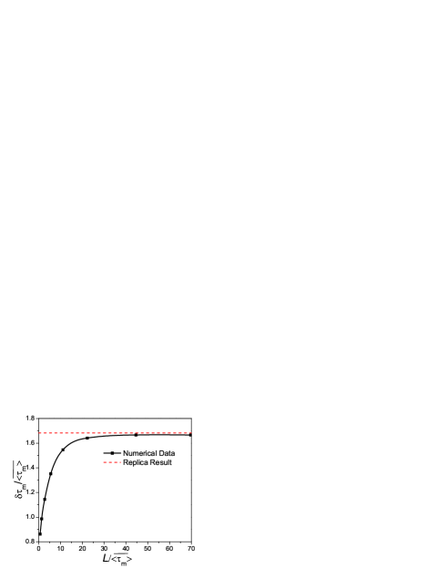
Figure 3: Dependence of the relative width of the distribution $\delta\tau_{m}/\overline{\langle\tau_{m}\rangle}$ on the system size. Symbols correspond to the actual data, the solid line is the guide to the eye, and the dashed line corresponds to the replica result in the thermodynamic limit.

It is obvious from the figure that in the thermodynamic limit $L\to\infty$ the replica result is in excellent agreement with numerical simulations. We mention that numerical simulations of $\delta\tau_{m}$ show very strong finite size effects. Therefore one has to go to very large $L\gtrsim 50\overline{\langle\tau_{m}\rangle}$ in order to approach the thermodynamic limit for the width of the distribution.

Depending on the system the quantity $\overline{\langle\tau_{m}^{2}\rangle}$ is not always experimentally accessible. For example, in the unzipping experiments it is easier to measure thermal average, $\langle\tau_{m}\rangle$, in each experimental run. We note that this quantity has sample to sample fluctuations only due to the presence of disorder. Then the variance of the distribution will be characterized by $\overline{\langle\tau_{m}\rangle^{2}}$. The difference between the two expectation values is given by $w$ found in Eq. (33). Defining $(\delta\tau_{m}^{T})^{2}=\overline{\langle\tau_{m}\rangle^{2}}-\overline{\langle\tau_{m}\rangle}^{\,2}$ and using Eqs. (37) and (33) we find that $\delta\tau_{m}^{T}/\overline{\langle\tau_{m}\rangle}\approx\sqrt{\kappa/2}$ in the weak disorder limit ($\kappa\ll 1$) and $\delta\tau_{m}^{T}/\overline{\langle\tau_{m}\rangle}\approx\sqrt{3}-1/(\sqrt{3}\kappa)$ in the opposite limit $\kappa\gg 1$. We plot both $\delta\tau_{m}^{T}$ and $\delta\tau_{m}$ versus the disorder parameter $\kappa$ in Fig. 4.

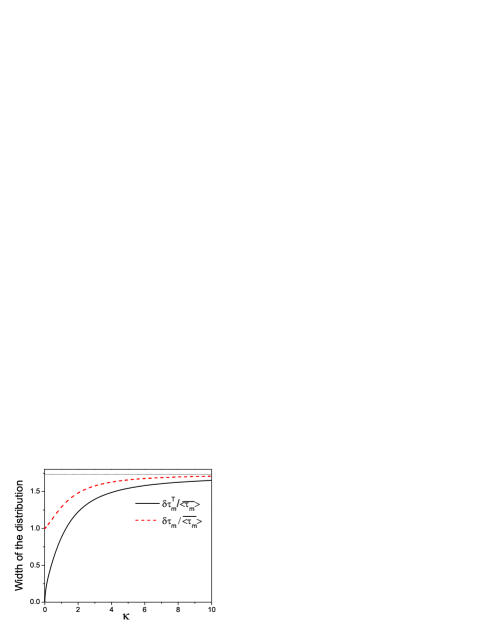
Figure 4: Dependence of the relative width of the distribution on the disorder parameter $\kappa$. The two curves correspond to different averaging over temperature and disorder (see text for details). The horizontal line at $\sqrt{3}$ denotes the asymptotic value of both $\delta\tau_{m}$ and $\delta\tau_{m}^{T}$ at $\kappa\to\infty$

The same issue of importance of the order of thermal and disorder averaging appears in the calculation of the higher moments of $\tau_{m}$, becoming irrelevant only in the limit ($\kappa\to\infty$), which effectively corresponds to the zero temperature case.

Before concluding this section let us make a few remarks about the rebinding transition, i.e., the rezipping that occurs with decreasing force. One can consider a similar setup with a lower end of the flux line fixed at the bottom of the columnar pin and the top end is pulled away from the pin with a force $f$. However, now we will be interested in $f>f_{c}$. Then clearly most of the flux line will be unzipped from the pin except for a portion near the bottom end. If $f$ is very large, the length of the bound segment $\tilde{\tau}_{m}$ near the sample boundary is small. However as $f$ decreases and approaches $f_{c}$ from above, the length of this segment increases and finally diverges at the transition. This rebinding transition can be described in a similar spirit to the unbinding. For example instead of the free energy (27) one has to deal with

$$\mathcal{F}(\tilde{\tau}_{m})=|\epsilon|\tilde{\tau}_{m}+\int_{0}^{\tilde{\tau}_{m}}d\tau_{m}^{\prime}U(\tau_{m}^{\prime}).$$ (41)

As we already noted the free energies (27) and (41) are equivalent up to an unimportant constant equal to the total disorder potential of the pin: $\int_{0}^{L}d\tau_{m}^{\prime}U(\tau_{m}^{\prime})$. We conclude that the unbinding and rebinding transitions for a single flux line on a disordered columnar pin are identical. In other words, statistical properties of $\tau_{m}$ for a given $f=f_{c}-\delta f$ are identical to those of $\tilde{\tau}_{m}$ for $f=f_{c}+\delta f$.

II.4 Unzipping from a planar defect without excursions.

We now generalize the ideas of the previous section to the more complicated problem of unzipping of a single flux line from a disordered twin plane. As before we ignore excursions out of the plane for the bound part of the flux line. Let us consider the rebinding transition first. That is we assume that $f$ is slightly greater than $f_{c}$ and we study the statistics of the bound part of the flux line. We again assume that the flux line is pinned at the bottom of the plane ($\tau=0$) and unbinds for $\tau$ larger than some $\tilde{\tau}_{m}$.

The point disorder potential now depends on the two coordinates $\tau$ and $z$ spanning the twin plane. Using Eq. (5) the partition function reads:

$$Z=\int_{0}^{L}d\tilde{\tau}_{m}\int Dz(\tau^{\prime})\exp\biggl{[}-{f^{2}\over 2\gamma}\tilde{\tau}_{m}-V\tilde{\tau}_{m}$$

$$~{}~{}~{}-\beta\int_{0}^{\tilde{\tau}_{m}}d\tau^{\prime}\left({\gamma\over 2}\left({dz\over d\tau^{\prime}}\right)^{2}+\mu(\tau^{\prime},z^{\prime})\right)\Biggr{]},$$ (42)

where $V<0$ is the mean attractive potential of the twin plane and we have dropped the unimportant $L$-dependent factors. As before, we assume a Gaussian random noise with zero mean and

$$\overline{\mu(\tau_{1},z_{1})\mu(\tau_{2},z_{2})}=\sigma\delta(\tau_{1}-\tau_{2})\delta(z_{1}-z_{2}).$$ (43)

We also introduce $\epsilon=-f^{2}/(2\gamma)-V$. Note that for the rebinding transition $\epsilon<0$. After replicating the partition function and averaging over point disorder we find

$$\overline{Z^{n}}=n!\int\limits_{0}^{L}d\tilde{\tau}_{n}\int\limits_{\tilde{\tau}_{n}}^{L}d\tilde{\tau}_{n-1}\ldots\int\limits_{\tilde{\tau}_{2}}^{L}d\tilde{\tau}_{1}\int Dz_{1}(\tau_{1}^{\prime})\dots Dz_{n}(\tau_{n}^{\prime})$$

$$~{}~{}~{}~{}~{}~{}~{}\exp\left[\sum_{\alpha=1}^{n}\epsilon\tilde{\tau}_{\alpha}+\!\!\!\int\limits_{\tilde{\tau}_{\alpha+1}}^{\tilde{\tau}_{\alpha}}\!\!\!d\tau_{\alpha}^{\prime}\mathcal{L}_{\alpha}[z_{1}(\tau_{1}^{\prime}),\ldots,z_{\alpha}(\tau_{\alpha}^{\prime})]\right],$$ (44)

where we define $\tilde{\tau}_{n+1}\equiv 0$ and $\mathcal{L}_{\alpha}$ is the Euclidean Lagrangian corresponding to the Hamiltonian ($\mathcal{H}_{\alpha}$) of $\alpha$ interacting particles Kardar :

$$\mathcal{H}_{\alpha}=-{\sigma\over 2}\alpha-{1\over 2\gamma}\sum_{\beta=1}^{\alpha}{\partial^{2}\over\partial z_{\beta}^{2}}-\sigma\sum_{1\leq\beta<\gamma\leq\alpha}\delta(z_{\beta}-z_{\gamma}).$$ (45)

Close to the rebinding transition, we anticipate $\tilde{\tau}_{m}\to\infty$ and thus the mean separation between the rebinding times of different replicas $\tilde{\tau}_{\alpha}$ and $\tilde{\tau}_{\alpha-1}$ diverges. Therefore the contribution to the partition function coming from integration over $\tau_{\alpha}$ will be dominated by the ground state of configurations with $\alpha$ replicas. In this case we can significantly simplify the partition function and evaluate it analytically:

$$\overline{Z^{n}}=n!\int\limits_{0}^{L}d\tilde{\tau}_{n}\int\limits_{\tilde{\tau}_{n}}^{L}d\tilde{\tau}_{n-1}\ldots\int\limits_{\tilde{\tau}_{2}}^{L}d\tilde{\tau}_{1}$$ (46)

$$\exp\left[\sum_{\alpha=1}^{n}\epsilon\tilde{\tau}_{\alpha}+(\mathcal{E}_{\alpha}-\mathcal{E}_{\alpha-1})\tilde{\tau}_{\alpha})\right].$$

Here $\mathcal{E}_{\alpha}$ is the ground state energy of $\mathcal{H}_{\alpha}$ with a subtracted term linear in $\alpha$, that just renormalizes $f_{c}$. Close to the transition $\epsilon$ is linear in the difference $f-f_{c}$. The energy, $\mathcal{E}_{\alpha}$, was computed in Ref. [Kardar, ]:

$$\mathcal{E}_{\alpha}=-{\sigma^{2}\gamma\over 12}\alpha^{3}=-\xi\alpha^{3}.$$ (47)

Upon integrating over $\tilde{\tau}_{\alpha}$ one obtains

$$\overline{Z^{n}}=n!\prod_{\alpha=1}^{n}{1\over|\epsilon|\alpha-\xi\alpha^{3}}\to\prod_{\alpha=1}^{n}{1\over|\epsilon|-\xi\alpha^{2}}$$ (48)

The product above can be reexpressed in terms of $\Gamma$-functions, which in turn allows for a straightforward analytic continuation to $n\to 0$:

$$\overline{Z^{n}}={1\over\xi^{n}}{1\over 1+n{\sqrt{\xi}\over\sqrt{|\epsilon|}}}{\Gamma\left({\sqrt{|\epsilon|}\over\sqrt{\xi}}-n\right)\over\Gamma\left({\sqrt{|\epsilon|}\over\sqrt{\xi}}+n\right)}.$$ (49)

Using this expression we obtain the free energy and the mean length of the localized segment:

$$\mathcal{F}=-\lim_{n\to 0}{\overline{Z^{n}}-1\over n}=\ln\xi+{\sqrt{\xi}\over\sqrt{|\epsilon|}}+2\Psi\left({\sqrt{|\epsilon|}\over\sqrt{\xi}}\right),$$ (50)

$$\overline{\langle\tilde{\tau}_{m}\rangle}={\partial\mathcal{F}\over\partial|\epsilon|}=-{\sqrt{\xi}\over 2|\epsilon|^{3/2}}+{1\over\sqrt{|\epsilon|\xi}}\Psi^{(1)}\left({\sqrt{|\epsilon|}\over\sqrt{\xi}}\right)$$ (51)

where as before $\Psi^{(n)}(x)$ stands for the $n$th derivative of the digamma function. This expression has the asymptotic behaviors:

$$\overline{\langle\tilde{\tau}_{m}\rangle}\to{1\over\epsilon}\qquad\quad~{}\xi\ll|\epsilon|$$

$$\overline{\langle\tilde{\tau}_{m}\rangle}\to{\sqrt{\xi}\over 2|\epsilon|^{3/2}}\quad\xi\gg|\epsilon|.$$ (52)

This scaling confirms the crossover between exponents $\nu=1$ and $\nu=3/2$ for the rebinding transition to a two-dimensional disordered plane predicted by the simple scaling argument leading to Eq. (21).

In a similar way one can also consider an unzipping transition with $f\leq f_{c}$. One finds an expression for the partition function which is identical to (48) with the substitution $\xi\to-\xi$. Note however, that the analytic continuation of the product (49) results in a complex partition function and hence a complex free energy. It thus appears that the analytic continuation of the product (48) to noninteger values of $n$ is not unique. One can always multiply it by any periodic function of $n$, which is equal to unity when the argument is integer. While we were able to find some real-valued analytic continuations of $\overline{Z^{n}}$ to negative values of $\xi$, these continuations did not lead to physically sensible results.

Because of the ambiguity of the analytic continuation and some approximations used to derive Eqs. (50) and (51) we also performed numerical simulations for the vortex unzipping from a disordered twin plane.

For numerical simulations we are using the lattice version of the model, where in each step along the $\tau$ direction the vortex can either move to the left or the right one lattice spacing. Note that because we neglect excursions the vortex motion occurs strictly within the plane until the vortex is unbound. Then the restricted partition function for the bound part of the flux line, $Z(x,\tau)$, which sums over the weights of all path leading to $x,\tau$, starting at $x=0,\tau=0$ satisfies the recursion relation Kardar

$$Z(x,\tau+1)=e^{\mu(x,\tau+1)}\big{[}JZ(x-1,\tau)+JZ(x+1,\tau)$$

$$~{}~{}~{}~{}~{}~{}~{}~{}~{}~{}~{}~{}~{}~{}~{}~{}~{}~{}~{}~{}~{}~{}~{}~{}~{}~{}~{}~{}~{}~{}+(1-2J)Z(x,\tau)\big{]}.$$ (53)

We assume that $\mu(x,\tau)$ is uniformly distributed in the interval $[-U_{0},U_{0}]$ implying as before the variance $\sigma=U_{0}^{2}/3$. The variable $J$ controls the line tension. In the continuum limit $J\ll 1$ and $U_{0}\ll 1$ the equation (53) reduces to the Schrödinger equation:

$${\partial Z\over\partial\tau}=-\mathcal{H}Z(x,\tau)$$ (54)

with the Hamiltonian given by Eq. (9) with $\gamma=2J$ and $f=0$ (there is no force acting on the flux line within the plane). We note that even if the parameters of the discrete model are not small we still expect that Eq. (54) remains valid at long length and time scales. However, the relation between the microscopic parameters of the discrete model and the parameters of the effective coarse-grained Hamiltonian (9) is more complicated.

In our simulations we evaluated numerically the free energy of the bound part of the vortex line for each realization of point disorder and used the analytical expression for the free energy of the unbound part, for which point disorder can be neglected. The latter is given by Eq. (5). This free energy is controlled by a single parameter $f^{2}/(2\gamma)$. Use of the analytic result (5) significantly simplifies calculations of $\overline{\langle\tau_{m}\rangle}$ and allows us to perform large scale simulations.

First we verify the scaling (20) with $\nu=3/2$ at the unzipping transition. To do this we perform standard finite size scaling procedure.

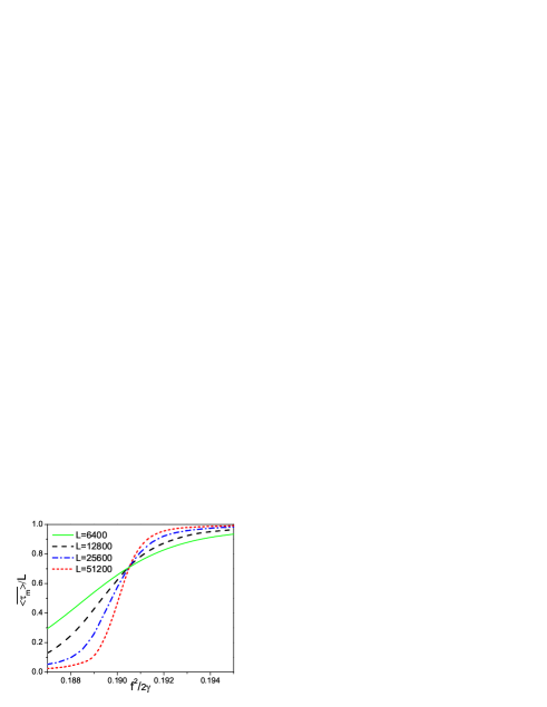
Figure 5: Ratio of the unzipping length $\overline{\langle\tau_{m}\rangle}$ to the system size $L$ as a function of $f^{2}/2\gamma$ for different system sizes. Here $f$ is the external force and $\gamma$ is the line tension of the vortex (see Eqs. (4 and (5))). According to the scaling relation (22) the crossing point corresponds to the unzipping transition. In simulations the parameters of the microscopic model (53) are chosen to be $J=0.2$, $U_{0}=2$

In Fig. 5 we show dependence of the ratio $\overline{\langle\tau_{m}\rangle}/L$ on the parameter $f^{2}/(2\gamma)$ for four different sizes. As we expect from the scaling relation (22) the three curves intersect at the same point corresponding to the unzipping transition ($g_{0}\approx 0.7$). Once we determine the crossing point corresponding to the critical force $f_{c}$ we can verify the scaling relation (22) with $\nu=3/2$.

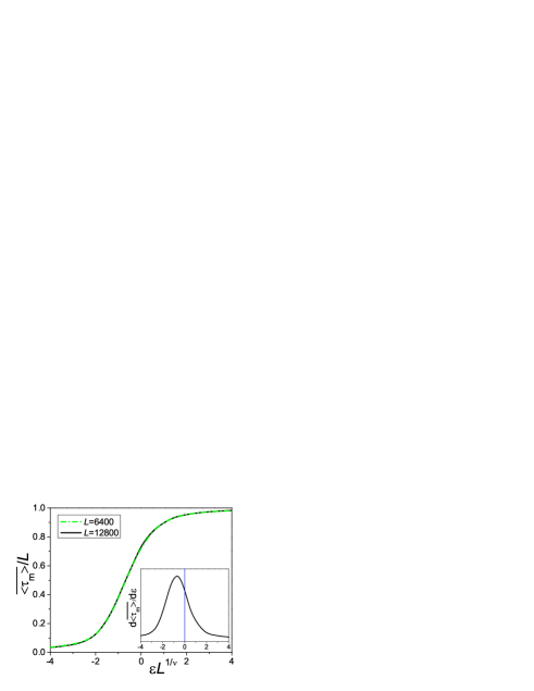
Figure 6: Data collapse of $\overline{\langle\tau_{m}\rangle}/L$ as a function of $\epsilon L^{1/\nu}$ with the exponent $\nu=3/2$ for two different system sizes (see Eq. (22)). The parameters of the model are the same as in Fig. 5. The inset shows derivative of $\overline{\langle\tau_{m}\rangle}$ with respect to $\epsilon$ for $L=12800$. Clearly the scaling function is asymmetric with respect to $\epsilon\to-\epsilon$. Thus the unbinding and rebinding transitions are not equivalent.

In Fig. 6 we plot $\overline{\langle\tau_{m}\rangle}/L$ versus the scaling parameter $\epsilon L^{1/\nu}$ (see Eq. (22)) with $\nu=3/2$ for two different system sizes. Clearly the data collapse is nearly perfect, which proves the validity of the scaling (63) with $\nu=3/2$ for the unzipping of a flux line from a twin plane. The inset shows the derivative of $\overline{\langle\tau_{m}\rangle}$ with respect to $\epsilon$. Clearly this derivative is asymmetric with respect to $\epsilon\to\ -\epsilon$, implying that there is no symmetry between the unbinding and rebinding transitions. This is contrary to the unzipping from a columnar pin with no excursions, where such a symmetry does exist.

Next we turn to verifying the analytic prediction for $\overline{\langle\tau_{m}\rangle}$, Eq. (51). As we argued above the parameter $\zeta$ describing the disorder strength can be easily extracted from microscopic parameters of the model only in the continuum limit $U_{0}\gg 1$, $J\ll 1$. Unfortunately, it is not possible to do simulations directly in the continuum limit ($J\ll 1$ and $U_{0}\ll 1$). Indeed as Eq. (51) suggests in order to see the scaling exponent $\nu=3/2$ one needs to go to length scales much larger than $1/\xi$, where $\xi=\sigma^{2}J/12=U_{0}^{4}J/36$. If $J\ll 1$ and especially $U_{0}\ll 1$ then one has to simulate extremely large system sizes where $L$ is larger than $10^{7}$ for $U_{0}=0.1$ and $J=0.1$. Therefore we perform simulations in the regime where $J$ and especially $U_{0}$ are appreciable. We then regard $\xi$ as a fitting parameter of the model which should be equal roughly to $U_{0}^{4}J/36$.

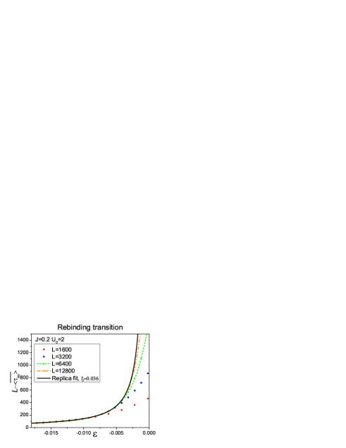
Figure 7: Dependence of the length of the bound part of the flux line to the twin plane $L-\overline{\langle\tau_{m}\rangle}$ on $\epsilon$ for the rebinding transition. Different curves correspond to different system sizes. The solid black line is the best single parameter fit using Eq. (51) with $\xi$ being the fitting parameter.

In Fig. 7 we show results of numerical simulation for the rezipping length $L-\overline{\langle\tau_{m}\rangle}$ on the detuning parameter $\epsilon$ for different system sizes. The solid black line is the best single-parameter fit to the data using the analytic expression (51). The fitting parameter $\xi$ found from simulations is $\xi\approx 0.036$, while a continuum estimate $U_{0}^{4}J/36$ gives $\xi\approx 0.089$, which is very reasonable given that this estimate is valid only at $U_{0}\ll 1$. We also performed similar simulations for $U_{0}=1.5$ and got a very good fit with (51) for $\xi=0.018$, while the continuum estimate gives $\xi\approx 0.028$. We thus see that indeed as $U_{0}$ decreases the fitting parameter $\xi$ becomes closer to the continuum expression.

While we were not able to derive a closed analytic expression for $\overline{\langle\tau_{m}\rangle}$ for the unbinding transition, we performed numerical simulations. As the inset in Fig. 6 suggests the transition is highly asymmetric. In fact this asymmetry persists in the thermodynamic limit.

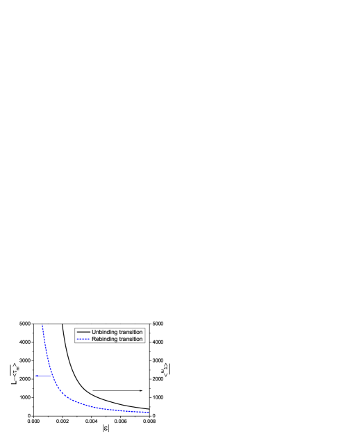
Figure 8: Comparison of dependences of $L-\overline{\langle\tau_{m}\rangle}$ for the rebinding transition and $\overline{\langle\tau_{m}\rangle}$ for the unbinding transition on $|\epsilon|$. We used the parameters of Fig. 5 with $L=51200$. The finite size effects are negligible on the scale of the graph. Both curves interpolate between $1/|\epsilon|$ dependence at $|\epsilon|\gg\xi$ and $C/|\epsilon|^{3/2}$ at $|\epsilon|\ll\xi$. However, the prefactor $C$ for the unbinding transition is about three times larger than for the rebinding.

In Fig. 8 we plot $L-\overline{\langle\tau_{m}\rangle}$ for the rebinding transition and $\overline{\langle\tau_{m}\rangle}$ for the unbinding versus $|\epsilon|$. Both curves interpolate between $1/|\epsilon|$ dependence at weak disorder $|\epsilon|\ll\xi$ and $C/|\epsilon|^{3/2}$ dependence at strong disorder $|\epsilon|\gg\xi$. However, the prefactor $C$ in front of $1/|\epsilon|^{3/2}$ is larger for the unzipping transition.

II.5 Unzipping from a hard wall

As the next step we consider unzipping from an attractive hard wall in $d=1+1$ dimensions with point disorder in the bulk. Our method is a straightforward generalization of the Bethe ansatz solution found by Kardar in the absence of the external force Kardar . The system is illustrated in Fig. 9. Here the potential experienced by the flux line, $V(x)$, has a short ranged attractive part and an impenetrable core at $x=0$. While the scaling argument is unchanged in this case, this problem has the merit of being exactly solvable within the replica approach. Since most details of the calculation are identical to those presented in Ref. [Kardar, ], here we only outline the solution.

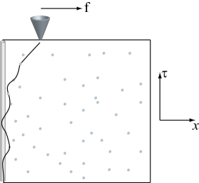
Figure 9: An illustration of the setup considered in the Bethe Ansatz calculation. The flux line is restricted to the half plane and a MFM tip is acting on it at the top of the sample.

After replicating the free energy Eq. (13) along with the contribution from the external field Eq. (2) and averaging over the disorder, the replicated sum over all path weights connecting points $(0,0)$ and $(x,\tau)$, $\overline{Z^{n}(x,t)}$, can be calculated from

$$\partial_{\tau}\overline{Z^{n}(x,t)}=-{\cal H}\overline{Z^{n}(x,t)}\;,$$ (55)

with the initial condition $\overline{Z^{n}(x,0)}=\delta(x)$. The replicated system describes $n$ attractively interacting bosons with a non-Hermitian Hamiltonian ${\cal H}$ given by

$${\cal H} = \sum_{\alpha=1}^{n}\left[-\frac{1}{2\gamma}\partial^{2}_{x_{\alpha}}-f\partial_{x_{\alpha}}+V(x_{\alpha})\right]$$ (56)

$$- \sigma\sum_{\alpha<\beta}\delta(x_{\alpha}-x_{\beta})-\frac{1}{2}\sigma n\;.$$

In Ref. [Kardar, ] the problem was solved for $f=0$ using the Bethe Ansatz. The boundary conditions were that the ground state wave function should vanish at large $x$ should decay as $\exp(-\lambda x)$ for the particle closest to the wall. One then finds that for the permutation ${\bf P}$ of particles such that $0<x_{P1}<x_{P2}<\ldots<x_{Pn}$ the wave function for $f=0$ is

$$\Psi_{f=0}\sim\exp\left(-\sum_{\alpha=1}^{n}\kappa_{\alpha}x_{P\alpha}\right)\;.$$ (57)

Here $\kappa_{\alpha}=\lambda+2(\alpha-1)\kappa$, $\kappa=\sigma\gamma/2$. Taking the zero replica limit it was found Kardar that for weak disorder ($\sigma\gamma/2<\lambda$) the vortex is bound to the wall while for strong disorder ($\sigma\gamma/2>\lambda$) it is unbound.

The ground state wave function for the non-zero value of the force can be obtained by noting that the non-Hermitian term acts like an imaginary vector potential. In particular, it can be gauged away when the vortices are bound to the wall as discussed in Sec. II.1 (see Eqs. (10) and (11)). This imaginary gauge transformation gives

$$\Psi_{f}=\Psi_{f=0}\exp\left(\sum_{\alpha=1}^{n}fx_{\alpha}\right)\;,$$ (58)

which implies that the solution is

$$\Psi_{f}=\exp\left(-\sum_{\alpha=1}^{n}\tilde{\kappa}_{\alpha}x_{P\alpha}\right)\;,$$ (59)

with $\tilde{\kappa}_{\alpha}=\lambda+2(\alpha-1)\kappa-f$. The effect of the force is simply to shift all the $\kappa_{\alpha}$’s by a constant. The average localization length (which satisfies near the transition $\langle x_{m}\rangle\simeq f_{c}\langle\tau_{m}\rangle/\gamma$) is then given by

$$\langle x_{m}\rangle={1\over\tilde{Z}_{n}n}\int_{0}^{\infty}\prod_{j=1}^{n}dx_{j}\left[\sum_{j=1}^{n}x_{j}\right]\,\Psi_{f}(x_{j}),$$ (60)

where $\tilde{Z}_{n}=\int_{0}^{\infty}\prod_{j=1}^{n}dx_{j}\Psi_{f}(x_{j})$. Note that the normalization factor $\tilde{Z}_{n}$ in the equation above is formally equivalent to the partition function (29) for the unzipping from a columnar pin without excursions if we identify $\lambda-\kappa-f$ with $\epsilon$ and $\kappa$ with $\Delta/2$. This equivalence implies that $\langle x_{m}\rangle$ for the unzipping from a hard wall has the same statistical properties as $\overline{\langle\tau_{m}\rangle}$ for the unbinding from a columnar pin (for more details see Ref. [kp, ]). In particular, the unzipping problem has a crossover from $\langle x_{m}\rangle\sim 1/(f_{c}-f)$ for $\lambda-f\gg\kappa$ to $\langle x_{m}\rangle\sim 1/(f_{c}-f)^{3/2}$ in the opposite limit.

This example confirms another prediction of the simple scaling argument: the critical exponents for the unbinding transition are determined only by the dimensionality of the defect even if the disorder is also present in the bulk of the system.

II.6 Unzipping from a columnar pin with excursions into the bulk.

In this section we consider the setup similar to Sec. II.3, namely unzipping from a columnar defect in $d=1+1$ dimensions, but allowing excursions of the flux line to the bulk (see Fig. 10).

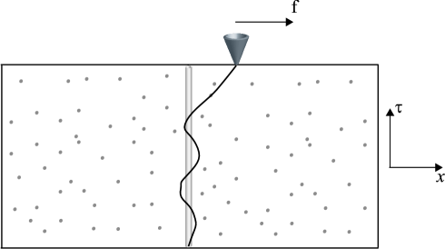
Figure 10: A setup illustrating unzipping from a columnar pin in $d=1+1$ dimensions with excursions into the bulk.

Unfortunately there is no analytic solution available for this problem. Therefore we present only numerical results. As in Sec. II.4 we consider a lattice version of the model where in each step along the $\tau$ direction the vortex can either move to the left or the right one lattice spacing. The attractive potential was placed at $x=0$. The restricted partition function of this model, $Z(x,\tau)$, which sums over the weights of all path leading to $x,\tau$, starting at $x=0,\tau=0$ satisfies the recursion relation Kardar :

$$Z(x,\tau+1)=\delta_{x,0}(e^{V}-1)Z(0,\tau)$$

$$+e^{\mu(x,\tau+1)}\left[Je^{f}Z(x-1,\tau)+Je^{-f}Z(x+1,\tau)\right].$$ (61)

Similarly to Eq. (53) we assume that $\mu(x,\tau)$ is uniformly distributed in the interval $[-U_{0},U_{0}]$ implying the variance $\sigma=U_{0}^{2}/3$. The variable $J$ controls the line tension, $V$ is the attractive pinning potential, and $f$ is proportional to the external force. In the continuum limit $J\ll 1$, $f\ll 1$, and $U_{0}\ll 1$, equation (61) reduces to the Schrödinger equation:

$${\partial Z\over\partial\tau}=-\mathcal{H}Z(x,\tau)$$ (62)

with the Hamiltonian given by Eq. (9) with $\gamma=2J$.

For the simulations we have chosen particular values of $J=0.1$ and $V=0.1$. As before we work in units such that $k_{B}T=1$. In the results described below the partition function was evaluated for each variance of the disorder for several systems of finite width $w=2L_{x}$ averaging over the time-like direction (typically $\tau\simeq 10^{6}$ “time” steps) with the initial condition $Z(0,0)=1$ and $Z(x,0)=0$ for $x\neq 0$.

To analyze the numerics we performed a finite size scaling analysis. In the spirit of Eq. (20), in the vicinity of the transition we expect the scaling form (compare Eq. (22)):

$$\overline{\langle\tau_{m}\rangle}=L_{x}\Phi\left[L_{x}(f_{c}-f)^{\nu}\right],$$ (63)

where $\Phi$ is some scaling function. Based on the results of previous sections we anticipate a smooth interpolation between scaling exponents $\nu=1$ and $\nu=2$ with either increasing $L_{x}$ or increasing strength of disorder at fixed $L_{x}$. To perform the finite size scaling we obtain for each value of $L_{x}$ a value for the exponent $\nu$ from the best collapse of the numerical data of two systems sizes $L_{x}$ and $L_{x}/2$. In Fig. 11 we plot $1/\nu$ as a function of the system size $L_{x}$. As can be seen the data is consistent with $\nu$ saturating at $\nu=2$ for large systems. The crossover to $\nu=2$ is much more rapid if the point disorder is enhanced near the columnar pin (see the inset in Fig. 11), as might be expected for damage tracks created by heavy ion radiation.

Figure 11: Effective exponent $1/\nu$ versus $L_{x}$ for a fixed strength of point disorder $\sigma=0.03$. The results are consistent with the general argument that this exponent should saturate at $\nu=2$ as $L_{x}\to\infty$. The inset shows the same exponent vs $\sigma_{c}$, the variance of additional point disorder placed directly on the columnar pin extracted from two system sizes $L_{x}=600$ and $L_{x}=1200$. It appears that $\nu\to 2$ as $\sigma_{c}$ increases.

Next, we test the behavior of the critical force as the disorder strength is increased. According to our discussion in Sec. II.2.3, we anticipate that in the absence of an external force the flux line is always bound to the pin in $1+1$ dimensions. This is in contrast with the problem of unzipping from the wall discussed in the previous section, where there is a critical strength of the disorder, $\sigma_{c}$, which leads to an unbinding transition for $f=0$. Note that the existence of a critical value of the disorder is a direct consequence (see discussion in Sec. II.2.3) of the excursions of the vortex from the defect which, as argued above, do not modify the critical behavior of the unzipping transition. The existence of a critical value of the disorder is therefore strongly dependent on the dimensionality of the problem.

In numerical simulations for each strength of disorder we determine the critical force plotting the ratio $\overline{\langle\tau_{m}\rangle}/L_{x}$ for two different sizes $L_{x}$ and using the scaling relation (63). Note that this ratio does not depend on $L_{x}$ at $f=f_{c}$ (see also the discussion in Sec. II.4). We checked that this is indeed the case. Upon repeating this procedure for different disorder strengths we obtain the dependence $f_{c}(U_{0})$ which is plotted in Fig. 12.

Figure 12: Critical force for unzipping from a columnar defect in $1+1$ dimensions as a function of the disorder strength.

The graph suggests that there is no unbinding transition at zero tilt at any strength of disorder consistent with the scaling argument presented in Sec. II.2.3 and those of Ref. [HwaNatter, ]. We point out that the strongest disorder shown in the graph $U_{0}=0.9$ required samples quite extended in the time-like direction, $L_{\tau}\approx 10^{8}$.

III Unzipping a Luttinger liquid

We now turn to consider the effect of interactions on the unzipping of single vortices. To do this we study a system where the vortices are preferentially bound to a thin two-dimensional slab which is embedded in a three-dimensional sample so that the density of vortices in the slab is much higher than in the bulk. Experimentally, this setup could be achieved using, for example, a twin plane in YBCO or by inserting a thin plane with a reduced lower critical field $H_{c1}$ (with, for example, molecular beam epitaxy) into a bulk superconductor. The scenario we analyze is one where a MFM is used to pull a single vortex out of the two-dimensional slab (see Fig. 13). The physics of the vortices confined to two dimensions is well understood and is analogous to a spinless Luttinger liquid of bosons (see, e.g. Ref. [AHNS, ]).

As we show below the dependence of the displacement of the vortex from the two-dimensional slab on the force exerted by the MFM depends on the physics of the two-dimensional vortex liquid which resides in the slab. Specifically, the critical properties of the unbinding transition depend on the “Luttinger liquid parameter” which controls the large-distance behavior of the vortex liquid. The experimental setup can thus be used to probe the two-dimensional physics of the vortices in the slab.

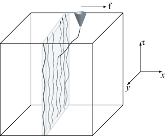
Figure 13: Possible experimental setup for studying unzipping from Luttinger Liquid. A MFM is used to pull a single vortex out of a plane where the vortices are confined. The measured quantity is the distance of the pulled vortex from the confining plane as a function of the force $f$.

III.1 Two-dimensional vortex liquids

The physics of vortices in two dimensions is very well understood. The vortices form a one-dimensional array located at position $x_{i}(\tau)$. The density profile of the vortices is then given by

$$n(x,\tau)=\sum_{j}\delta\left[x-x_{j}(\tau)\right]\;,$$ (64)

where $x$ and $\tau$ denote transverse and longitudinal coordinates with respect to the vortices and $i$ is an index labeling the vortices. By changing variable into the phonon displacement field $u_{j}$ through $x_{j}(\tau)=a\left[j+u_{j}(\tau)\right]$, where $a$ is the mean distance between vortex lines the free-energy of a particular configuration can be written as:

$${\cal F}_{0}=\frac{a^{2}}{2}\int dxd\tau\left[c_{11}(\partial_{x}u)^{2}+c_{44}(\partial_{\tau}u)^{2}\right]\;.$$ (65)

Here $c_{11}$ and $c_{44}$ are the compressional and the tilt moduli respectively. After rescaling the variables $x$ and $\tau$ according to

$$x\to x\left(\frac{c_{11}}{c_{44}}\right)^{1/4}\;\;,\;\tau\to\tau\left(\frac{c_{44}}{c_{11}}\right)^{1/4}\;,$$ (66)

the free energy takes the isotropic form

$${\cal F}_{0}=\frac{A}{2}\int dxd\tau\left[(\partial_{x}u)^{2}+(\partial_{\tau}u)^{2}\right]$$ (67)

with $A=a^{2}\sqrt{c_{11}c_{44}}$. The partition function is then given by the functional integral

$$Z=\int Du(x,\tau)e^{-S}\;,$$ (68)

with $S=S_{0}={\cal F}_{0}/T$. In the limit of large sample sizes in the “timelike” direction one can regard $Z$ as the zero temperature partition function of interacting bosons AHNS . In this language the imaginary time action can be written as

$$S_{0}=\frac{\pi}{2g}\int dxd\tau\left[(\partial_{x}u)^{2}+(\partial_{\tau}u)^{2}\right]\;.$$ (69)

Here we set $\hbar=1$ and identified the Luttinger-liquid parameter, $g$, as

$$g=\frac{\pi T}{A}\;.$$ (70)

The Luttinger-liquid parameter controls the long-distance properties of the model. For vortices $g$ it is a dimensionless combination of the compressional and tilt moduli, the density of vortices and temperature.

Various properties of Luttinger liquids are well understood. For example, the correlation function for the density fluctuations $\delta n(x,\tau)=n(x,\tau)-n_{0}$, where $n_{0}=1/a$ is the mean density, obeys

$$\langle\delta n(x,\tau)\delta n(0,0)\rangle\simeq\frac{\cos\left(2\pi n_{0}x\right)}{(x^{2}+\tau^{2})^{g}}\;.$$ (71)

There is quasi long-range order in the system and the envelope of the density correlation function decays as a power law with the exponent depending only on $g$. As we show below, $g$ can be probed by unzipping a single vortex out of a plane which contains a $(1+1)$-dimensional vortex liquid.

In what follows we also consider the case where there is point disorder present in the sample. The behavior will be strongly influenced by the behavior of the vortices in two dimensions in the presence of disorder. This problem has been studied in some detail in the past (see e.g. Ref. [pkn, ] and references therein). Here we briefly review features which will be important in analyzing the unzipping problem. The most relevant (in the renormalization group sense) contributions to the action from the point disorder is

$$S_{PD}=2\int dxd\tau R(x,\tau)\cos\left[2\pi u(x,\tau)+\beta(x,\tau)\right]\;,$$ (72)

where positive (negative) $R$ implies a repulsive (attractive) potential between the vortices and the quenched random disorder. We assume, for simplicity, that $\beta(x,\tau)$ is distributed uniformly between $0$ and $2\pi$ and $R(x,\tau)$ has a an uncorrelated Gaussian distribution with the variance $\Delta_{0}$:

$$\overline{R(x_{1},\tau_{1})R(x_{2},\tau_{2})}=\Delta_{0}\delta(x_{1}-x_{2})\delta(\tau_{1}-\tau_{2})\;,$$ (73)

where the overbar, as before, represents averaging over disorder.

To analyze the disordered problem, similar to the single vortex case, we use the replica trick. Then the replicated noninteracting part of the action becomes

$$S_{0}=\frac{\pi}{2g}\sum_{\alpha,\beta}\int\int dxd\tau\left[\frac{\partial u_{\alpha}}{\partial\tau}\frac{\partial u_{\beta}}{\partial\tau}+\frac{\partial u_{\alpha}}{\partial x}\frac{\partial u_{\beta}}{\partial x}\right]\left[\delta_{\alpha,\beta}-\frac{\kappa}{g}\right]\;.$$ (74)

Here $u_{\alpha}(x,\tau)$ is the replicated phonon field and $\kappa$ is an off-diagonal coupling which is zero in the bare model but is generated by the disorder. It plays the role of a quenched random “chemical potential” which is coupled to the first derivative of the phonon field $u$. The replica indices, $\alpha$ and $\beta$ run from $1$ to $n$ and at the end of the calculation one takes the limit $n\to 0$. After replication the contribution from the point disorder becomes

$$S_{PD}=-\Delta_{0}\sum_{\alpha,\beta}\int\int dxd\tau\cos 2\pi\left[u_{\alpha}(x,\tau)-u_{\beta}(x,\tau)\right]\;.$$ (75)

The combined action can be treated within the renormalization group using a perturbation series near $g=1$ where a phase transition between a vortex liquid and a vortex glass occurs fisher_v_glass . By continuously eliminating degrees of freedom depending on frequency and momentum within the shell $\Lambda-\delta\Lambda<\sqrt{\omega^{2}+q^{2}}<\Lambda$, one obtains the following renormalization group equations Cardy ; pkn

$$\frac{dg}{dl} = 0$$ (76)

$$\frac{d\Delta}{dl} = 2(1-g)\Delta-2C\Delta^{2}$$ (77)

$$\frac{d\kappa}{dl} = C^{2}\Delta^{2}$$ (78)

Here $l$ is the flow parameter $\Lambda(l)=\Lambda e^{-l}$. $C$ is a non-universal constant which depends on the cutoff $\Lambda$. The equations are subject to the initial conditions $\kappa(l=0)=0$ and $\Delta(l=0)=\Delta_{0}$. Note that the Luttinger liquid parameter is not renormalized. Analyzing the flow equations it has been shown that in the vortex liquid phase ($g>1$) the correlation of the density fluctuation behaves in the vortex liquid phase as

$$\langle\delta n(x,\tau)\delta n(0,0)\rangle\simeq\frac{1}{(x^{2}+\tau^{2})^{g+\tilde{\kappa}/2}}\;,$$ (79)

where $\tilde{\kappa}$ is a nonuniversal exponent. In the glass phase ($g<1$) correlations decay faster than a power law, with

$$\langle\delta n(x,\tau)\delta n(0,0)\rangle\simeq\exp\left(-(1-g)^{2}\ln^{2}\sqrt{x^{2}+\tau^{2}}\right)\;.$$ (80)

In what follows we consider a setup in which a two dimensional array of vortices, whose properties have been described above, is embedded in a three dimensional bulk sample. As shown below when a single vortex is unzipped into the bulk in a clean sample the critical properties of the unzipping transition yield information on the properties of the two dimensional vortex liquid. In particular, they provide a direct measure of the Luttinger-liquid parameter. In the same setup in a disordered sample we will show that the critical properties of the unzipping transition will be modified. In particular, they can yield information on the on the three-dimension wandering exponent of a single vortex in a disordered sample.

III.2 Unzipping a Luttinger liquid: The clean case

Consider first an experiment where an attractive two-dimensional potential holds vortices confined to it. A MFM then pulls a single vortex out of the plane (see Fig. 13). We assume throughout that the density of vortices in the three dimensional bulk is so small that we can neglect interactions between the vortex that is pulled out of the sample and vortices in the three dimensional bulk. In this subsection only the clean case (no point disorder) will be studied.

We assume the MFM exerts a force ${\bf f}=f\hat{x}$. As in the unzipping experiments discussed above we expect that for large forces $f>f_{c}$ the vortex will be completely pulled out of the two dimensional slab. Similar to the case of the unzipping of a single vortex we write the free energy of the vortex as a sum of two contributions. The first, ${\cal F}_{u}(\tau_{m})$, arises from the part of the vortex that is outside the two dimensional slab. The second ${\cal F}_{b}(\tau_{m})$ is the change in the free-energy of the vortices that remain inside the two dimension slab. As before $\tau_{m}$ is the length along the $\tau$ direction which is unbound from the two-dimensional slab. The free-energy of the unzipped part is clearly identical to that calculated in Eq. 5 or explicitly

$${\cal F}_{u}(\tau_{m})=-f^{2}\tau_{m}/2\gamma\;.$$ (81)

The calculation of the free-energy, ${\cal F}_{b}(\tau_{m})$, is somewhat more involved. Clearly there is a linear contributions due to the length $\tau_{m}$ removed from the attractive potential of the slab. However, in addition there is an extra contribution from the energy of the dislocation, ${\cal F}_{d}(\tau_{m})$, (see Fig. 13) created in the two dimensional vortex array. This contribution to the free-energy, as we show below, is non-linear and controlled by the Luttinger liquid parameter $g$. This non-linearity results, near the unzipping transition, in a sensitivity of the critical properties to the value of $g$.

We leave the details of the calculation of the dislocation energy to Appendix A and present here only the key steps of derivation.

In order to satisfy boundary conditions near the interface one can use the method of images (see Fig. (15)). The free energy of this dislocation pair can be calculated by standard methods (see details in Appendix A). In particular, at large $\tau_{m}$ it behaves logarithmically (see e.g. Ref. [chakin, ]):

$${\cal F}_{d}=\frac{T}{4g}\ln(\tau_{m}/a_{0}),$$ (82)

where $a_{0}$ is the short range cutoff of the order of the distance between flux lines. We note that the free energy of the dislocation near the interface (82) is one half of the free energy of a dislocation pair.

With the energy of the dislocation in hand we can now analyze the properties of the unzipped length near the transition using the methods used for analyzing the single vortex unzipping experiments. The contributions to the free energy are from the unzipped part of the vortex and the energy of the dislocation. Collecting all the relevant terms, near the transition the free energy is given by

$${\cal F}(\tau_{m})={\cal F}_{u}(\tau_{m})+{\cal F}_{b}(\tau_{m})=\epsilon\tau_{m}+\frac{T}{4g}\ln(\tau_{m}/a_{0})\;.$$ (83)

The probability of finding a certain value of $\tau_{m}$ is then given by

$$P(\tau_{m})\propto e^{-F(\tau_{m})/T}=\frac{C}{\tau_{m}^{1/(4g)}}e^{-\epsilon\tau_{m}}.,$$ (84)

where $C$ is the normalization constant. At the transition $\epsilon=0$ the distribution becomes a pure power law in $\tau_{m}$. Therefore, the average value of $\tau_{m}$ is very sensitive to the value of $g$. In particular, for $g>1/4$ (i.e. for weakly interacting flux lines) the behavior of $\langle\tau_{m}\rangle$ near the transition is identical to that of a single vortex in the absence of interactions with other vortices

$$\langle\tau_{m}\rangle\sim{1\over\epsilon}\;.$$ (85)

In contrast, for $1/8<g<1/4$ (stronger interactions) there is a continuously varying exponent governing the transition

$$\langle\tau_{m}\rangle\sim{1\over\epsilon^{2-1/4g}}\;.$$ (86)

And finally, for $g<1/8$ (strongly interacting flux lines) we find that $\langle\tau_{m}\rangle$ does not diverge near the transition. Note that even though in this regime the mean displacement remains constant at the transition the higher moments of $\tau_{m}$ diverge and are thus sensitive to $\epsilon$. The reason for this is at the transition the distribution of $\tau_{m}$ is a power law.

III.3 Unzipping from a twin plane with point disorder

We now consider the problem of unzipping a vortex from a plane with many vortices in the presence of disorder. In the spirit of the treatments presented in this paper, one needs to calculate the free-energy of the unzipped part of the vortex ${\cal F}_{u}(\tau_{m})$, the free-energy of the bound part of the vortex ${\cal F}_{b}(\tau_{m})$ and the fluctuations in both quantities averaged over realizations of disorder. This can be done perturbatively near $g=1$. We again relegate details of the derivation of the dislocation energy to Appendix B. One conclusion from our calculations is that the mean free energy of the dislocation near the boundary is not affected by the disorder and is given by Eq. (82). Another important conclusion is that the fluctuations of the free energy also depend logarithmically on $\tau_{m}$:

$$\overline{\delta{\cal F}^{2}_{d}(\tau_{m})}=T^{2}\frac{\kappa(\infty)}{8g^{2}}\ln(\tau_{m}/a_{0})$$ (87)

for $g>1$ and

$$\overline{\delta{\cal F}^{2}_{d}(\tau_{m})}=T^{2}\frac{(1-g)^{2}}{4}\ln^{2}(\tau_{m}/a_{0})$$ (88)

for $g<1$.

Figure 14: Possible experimental setup for studying unzipping from Luttinger Liquid in the presence of disorder.

We note that in the case of many flux lines there is a weak logarithmic dependence of free energy fluctuations on $\tau_{m}$ as opposed to strong power law dependence in the case of a single flux line (compare Eq. (14)). This somewhat surprising result is a consequence of the screening of strong power-law fluctuations by other flux lines. We note that if the pinning of flux lines by disorder is extremely strong so that tearing a single flux line does not affect positions of other lines in the duration of experiment, we are back to the single flux line physics and $\overline{\delta\mathcal{F}_{d}^{2}}\propto\tau_{m}$.

To complete the analysis, we need to consider the free-energy contribution from the unzipped part. Of particular of importance are the free-energy fluctuations due to the disorder in the bulk of the sample. As discussed in Sec. II, in a three dimensional sample these grow as $\delta{\cal F}_{u}\propto m^{\omega(3)}$ with $\omega(3)\simeq 0.22$. This contribution grows much quicker than the contribution from the fluctuations in the free-energy of the dislocation. Therefore following the ideas of Sec. II the total free-energy is given by

$${\cal F}(m)=a(f_{c}-f)\tau_{m}-b\tau_{m}^{\omega(3)}\;.$$ (89)

where $a$ and $b$ are positive constants. Minimizing Eq. (89) gives for the critical properties in this case

$$s\sim\frac{1}{(f_{c}-f)^{1.28}}\;.$$ (90)

Thus screening disorder fluctuations in the plain by other flux lines effectively enhances the role of disorder in the bulk. As the result these unzipping experiments can serve as a probe of the three-dimensional anomalous wandering exponent.

Appendix A Calculation of the dislocation energy near the interface.

To calculate the energy of the dislocation created by unzipping in Fig. 13, standard methods can be used with a slight modification. The need for a modification is due to the requirement that vortex lines must exit normal to the interface of the superconductor at the top of the sample which ensures that the supercurrents are confined to the sample. One then has to sum over phonon field configuration, $u_{d}(x,\tau)$, which satisfy

$$\left.\frac{\partial u_{d}(x,\tau)}{\partial\tau}\right|_{\tau=0}=0\;.$$ (91)

Here, we have chosen the upper boundary of the two-dimensional slab to be located at $\tau=0$. The calculation can then be done using the method of images, depicted in Fig. 15, by writing the constrained field $u_{d}(x,\tau)$ in terms of an unconstrained field $u(x,\tau)$

$$u_{d}(x,\tau)=u(x,\tau)+u(x,-\tau)\;,$$ (92)

and summing over all configurations of the unconstrained field. In terms of the constrainted field the action is

$$S=\frac{\pi}{2g}\int_{-\infty}^{0}d\tau\int_{-\infty}^{\infty}dx\left[(\partial_{x}u_{d}(x,\tau))^{2}+(\partial_{\tau}u_{d}(x,\tau))^{2}\right]\;,$$ (93)

which rewritten in terms of the unconstrained field becomes

$$S = \frac{\pi}{2g}\int_{-\infty}^{\infty}d\tau\int_{-\infty}^{\infty}dx\left[(\partial_{x}u(x,\tau))^{2}+(\partial_{\tau}u(x,\tau))^{2}\right.$$ (94)

$$+ \left.\partial_{x}u(x,\tau)\partial_{x}u(x,-\tau)+\partial_{\tau}u(x,\tau)\partial_{\tau}u(x,-\tau)\right]\;.$$

In terms of the partial Fourier transform

$$u(x,\tau)=\frac{1}{(2\pi)^{1/2}}\int d\omega e^{i\omega\tau}u(x,\omega)\;,$$ (95)

the action becomes

$$S=\frac{\pi}{2g}\int_{-\infty}^{\infty}d\omega\int_{-\infty}^{\infty}dx\left[(\partial_{x}u^{\prime}(x,\omega))^{2}+\omega^{2}(u^{\prime}(x,\omega))^{2}\right]$$ (96)

where $u^{\prime}(x,\omega)$ is the real part of $u(x,\omega)$. The spatial Fourier transform

$$u^{\prime}(x,\omega)=\frac{1}{(2\pi)^{1/2}}\int dqe^{iqx}u^{\prime}(q,\omega)\;,$$ (97)

then finally gives

$$S=\frac{\pi}{2g}\int_{-\infty}^{\infty}dq\int_{-\infty}^{\infty}d\omega\left[(q^{2}+\omega^{2})|u^{\prime}(q,\omega)|^{2}\right]\;.$$ (98)

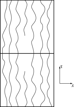
Figure 15: An illustration of configurations of the phonon field considered by the method of images.

Eq. 98 allows a straightforward calculation of the energy of a dislocation near the upper boundary of the slab (see Fig. 15) using standard tools. We use the correlation function Schultz

$$G(\tau_{m})=\left\langle e^{i\left[\phi(x,\tau_{m})-\phi(x,-\tau_{m})\right]}\right\rangle$$ (99)

where the boson phase angle $\phi$ is conjugate to $du/dx$. Here $m$ is, as before, the length of the unzipped segment and the angular brackets denote an average with respect to the action Eq. 98. In terms of this correlation function the free-energy of the dislocation is given by

$${\cal F}_{d}(\tau_{m})=-\frac{T}{2}\ln G(\tau_{m})\;,$$ (100)

where $T$ is the temperature and we have set, as before, the Boltzmann constant to be $k_{B}=1$. Note that we are interested in the correlation function of the unconstrained field $u(x,\tau)$. The factor of one-half originates from the fact that the we are interested in the energy up to $\tau=0$ and not between $-m$ and $m$. Integrating out the field $\phi$ in the standard way it is easy to show that this expression can be rewritten as

$$G(\tau)=\left\langle\exp\left(-\frac{i\pi}{g}\int_{-\tau_{m}}^{\tau_{m}}\partial_{x}u(0,\tau)d\tau\right)\right\rangle$$ (101)

It is then straightforward to find that for large $m$

$${\cal F}_{d}=\frac{T}{4g}\ln(\tau_{m}/a_{0})$$ (102)

where $a_{0}$ is a microscopic cutoff. The result turns out to be identical to that which would have been obtained without the constraint on the fields.

Appendix B Calculation of the dislocation energy in the presence of disorder

As in the clean sample we consider the correlation function

$$G(\tau_{m})=\left\langle\exp\left(-\frac{i\pi}{g}\int_{-\tau_{m}}^{\tau_{m}}\partial_{x}u(0,\tau)d\tau\right)\right\rangle$$ (103)

Note that in the clean case the method of images guaranteed that the flux lines exit normal to the interface. However, with disorder this will be the case only if disorder in the top image plane is correlated with the disorder in the bottom plane. However, we expect that at large $\tau_{m}$ these correlations will not be important and we will ignore them.

To obtain the free-energy with disorder and sample-to-sample fluctuations we consider the replicated correlation function $\overline{G(\tau_{m})^{n}}$. This allows the extraction of the disorder averaged free-energy from

$$\overline{{\cal F}_{d}(\tau_{m})}=T\frac{\partial}{\partial n}\overline{G(\tau_{m})^{n}}|_{n=0}$$ (104)

and the fluctuations in it from

$$\overline{\delta{\cal F}^{2}_{d}(\tau_{m})}=T^{2}\frac{\partial^{2}}{\partial n^{2}}\overline{G(\tau_{m})^{n}}|_{n=0}-T^{2}\left(\frac{\partial}{\partial n}\overline{G(\tau_{m})^{n}}|_{n=0}\right)^{2}$$ (105)

Using standard methods it is straightforward to obtain

$$\overline{G(\tau_{m})^{n}} = \exp\left(-\frac{1}{2g^{2}}\left[n\int_{0}^{\infty}dlg(1-J_{0}(\tau_{m}e^{-l}/a_{0}))\right.\right.$$ (106)

$$+ \left.\left.n^{2}\int_{0}^{\infty}dl\kappa(l)(1-J_{0}(\tau_{m}e^{-l}/a_{0}))\right]\right)\;,$$

where $a_{0}$ is a microscopic cutoff. The Bessel function $J_{0}(x)$ appearing in Eq. 106 and below is non-universal and depends on the details of the cutoff procedure. Combining this with the solutions of the flow equations yields

$$\overline{{\cal F}_{d}(\tau_{m})}=\frac{T}{4g}\ln(\tau_{m}/a_{0})\;.$$ (107)

Here we have included a factor of one-half since vortices exist in the lower half plane. The disordered free energy of the dislocation is the same as that of a dislocation in the clean sample. Similarly one can obtain for the free-energy fluctuations of the dislocation

$$\overline{\delta{\cal F}^{2}_{d}(\tau_{m})}=T^{2}\frac{\kappa(\infty)}{8g^{2}}\ln(\tau_{m}/a_{0})$$ (108)

for $g>1$ and

$$\overline{\delta{\cal F}^{2}_{d}(\tau_{m})}=T^{2}\frac{(1-g)^{2}}{4}\ln^{2}(\tau_{m}/a_{0})$$ (109)

for $g<1$.

As discussed in Sec. III.3 a crucial input from the above calculation is that the free-energy fluctuations grow at most logarithmically in $\tau_{m}$.

References

- (1) G. Blatter, M. V. Feigel’man, V. B. Geshkenbein, A. I. Larkin, and V. M. Vinokur, Rev. Mod. Phys. 66, 1125 (1994).
- (2) D.R. Nelson and H.S. Seung, Phys. Rev. B 39, 9153 (1989).
- (3) D. R. Nelson and V. M. Vinokur, Phys. Rev. B 48, 13060 (1993).
- (4) D. S. Fisher, M. P. A. Fisher and D. A. Huse, Phys. Rev. B 43, 130 (1991).
- (5) T. Giamarchi and P. Le Doussal, Phys. Rev. B 52, 1242 (1995); see also T. Natterman, Phys. Rev. Lett. 64, 2454 (1990).
- (6) A. Wadas, O. Fritz, H. J. Hug and H. J. Güntherodt, Z. Phys. B 88, 317 (1992).
- (7) For an overview see C. Bustamante, Z. Bryant, S. B. Smith, Nature 421, 423 (2003).
- (8) C. J. Olson Reichhardt and M. B. Hastings, Phys. Rev. Lett. 92, 157002 (2004).
- (9) Y. Kafri, D. Nelson, and A. Polkovnikov, Europhys. Lett. 73, 253 (2006).
- (10) C. A. Bolle et. al., Nature 399, 43 (1999).
- (11) N. Hatano and D.R. Nelson, Phys. Rev. B 56, 8651 (1997).
- (12) D.K. Lubensky and D.R. Nelson, Phys. Rev. Lett. 85, 1572 (2000), Phys. Rev. E 65, 031917 (2002).
- (13) D. R. Nelson, Defects and Geometry in Condensed Matter Physics, (Cambridge, UK, 2002).
- (14) I. Affleck, W. Hofstetter, D.R. Nelson, and U. Schollwöck, J. Stat. Mech.: Theor. Exp. P10003 (2004).
- (15) D. Marenduzzo, A. Trovato and A. Maritan, Phys. Rev. E 64, 031901 (2001).
- (16) E. Orlandini, M.C. Tesi and S.G Whittington, J. Phys. A: Math. Gen. 34, 1535 (2004).
- (17) For a review see for example M. Kardar in Fluctuating Geometries in Statistical Mechanics and Field Theory, Les Houches Summer School (1994, Springer).
- (18) T. Hwa and D. S. Fisher, Phys. Rev. B 49, 3136 (1994).
- (19) We note however, that because the relation (16) is not exact for higher dimensional defects, there is no symmetry between unzipping and rezipping transitions, i.e. and is the symmetry of the problem only for 1D columnar defects. See also Sec. II.6.
- (20) M. Opper, J. Phys. A 26, L719 (1993).
- (21) See for example V. Privman in Finite Size Scaling and Numerical Simulation of Statistical Systems, edited by V. Privman, World Scientific, Singapore (1990).
- (22) M. Kardar, Phys. Rev. Lett. 55, 2235 (1985).
- (23) M. Zapatocky and T. Halpin-Healy, Phys. Rev. Lett. 67, 3463 (1991).
- (24) L. -H. Tang and I. F. Lyuksyutov, Phys. Rev. Lett. 71, 2745 (1993).
- (25) L. Balents and M. Kardar, Europhys. Lett. 23, 503 (1993).
- (26) E. B. Kolomeisky and J. P. Staley, Phys. Rev. B 46, 12664 (1992).
- (27) L. Balents and M. Kardar, Phys. Rev. B, 49, 13030 (1994).
- (28) T. Hwa and T. Nattermann, Phys. Rev. B 51, 455 (1995).
- (29) Y. Kafri and A. Polkovnikov, Phys. Rev. Lett. 97, 208104 (2006).
- (30) S. F. Edwards and P. W. Anderson, J. Phys. F: Metal Phys. 5, 965 (1975).
- (31) M. Kardar, Nucl. Phys. B 290, 582 (1987).
- (32) P. le Doussal, C. Monthus, and D. S. Fisher, Phys. Rev. E 59, 4795 (1999).
- (33) A. Polkovnikov, Y. Kafri, and D. R. Nelson, Phys. Rev. B 71, 014511 (2005).
- (34) M.P.A. Fisher, Phys. Rev. Lett. 62, 1415 (1989).
- (35) T. Hwa and D. S. Fisher, Phys. Rev. Lett. 72, 2466 (1994), and references therein.
- (36) P. M. Chaikin and T. C. Lubensky, Principles of Condensed Matter Physics, (Cambridge, UK, 1995).
- (37) H. J. Schultz, B. I. Halperin and C. L. Henley, Phys. Rev. B 26, 3797 (1982).