Astrophysical interpretation of the medium scale clustering in the ultrahigh energy sky

Abstract

We compare the clustering properties of the combined dataset of ultra-high energy cosmic rays events, reported by the AGASA, HiRes, Yakutsk and Sugar collaborations, with a catalogue of galaxies of the local universe (redshift $z\lesssim 0.06$). We find that the data reproduce particularly well the clustering properties of the nearby universe within $z\lesssim 0.02$. There is no statistically significant cross-correlation between data and structures, although intriguingly the nominal cross-correlation chance probability drops from ${\cal O}$(50%) to ${\cal O}$(10%) using the catalogue with a smaller horizon. Also, we discuss the impact on the robustness of the results of deflections in some galactic magnetic field models used in the literature. These results suggest a relevant role of magnetic fields (possibly extragalactic ones, too) and/or possibly some heavy nuclei fraction in the UHECRs. The importance of a confirmation of these hints (and of some of their implications) by Auger data is emphasized.

I Introduction

One of the keys towards the solution of the mysterious origin of ultra-high energy cosmic rays (UHECRs) is the study of their anisotropy pattern. The chances to perform (some kind of) UHECR astronomy increase significantly at extremely high energy, in particular due to the decreasing of deflections in the galactic and possibly extragalactic magnetic fields. Moreover, at $E\gtrsim(4-5)\times 10^{19}\,$ eV the opacity of the interstellar space to protons drastically grows due to the kinematically allowed photo-pion production on Cosmic Microwave Background (CMB) photons, known as the Greisen-Zatsepin-Kuzmin or GZK effect Greisen:1966jv ; Zatsepin:1966jv . A similar phenomenon at slightly different energies occurs for heavier primaries via photo-disintegration energy losses. Recently, an observational evidence for a flux suppression consistent with the GZK feature has been reported by the HiRes collaboration Abbasi:2007sv . Within reasonable astrophysical assumptions, these energy-losses phenomena impose a conservative upper limit to the distance from which the bulk of UHECRs is emitted, of the order of a few hundreds Mpc at most, which may enhance the chances of identifying structures. In Ref. Cuoco:2005yd a forecast analysis for the Pierre Auger Observatory Auger ; Abraham:2004dt was performed to derive the minimum statistics needed to test the “zeroth order” hypothesis that UHECRs trace the baryonic distribution in the universe. Assuming proton primaries, it was found that a few hundred events at $E\gtrsim 5\times 10^{19}\,$eV are necessary at Auger to have reasonably high chances to identify the signature. On the other hand, available catalogues from the experiments of the previous generation contain ${\cal O}$(100) events above $E\gtrsim(4-5)\times 10^{19}\,$ eV, thus motivating a search for possible angular patterns already in the present data Anchordoqui:2003bx ; Kachelriess:2005uf . In particular, after renormalizing the energy scales of the different experiments to the HiRes one at $4\times 10^{19}$ eV, the authors of Kachelriess:2005uf found some evidence of a broad maximum of the two-point autocorrelation function of UHECR arrival directions around 25 degrees. Since the search was made a posteriori, the assessment of its significance is a delicate issue and involves the determination of a penalty factor critically dependent on the performed number of trials. The previous claim of small scale clustering in the AGASA data and the associated debate on its significance (see e.g. Takeda:1999sg ; Tinyakov:2001ic ; Finley:2003ur ) would suggest to take a cautionary attitude towards a posteriori claims. However, a similar feature has been found in the Auger data alone as well, as recently reported in Mollerach:2007vb . We shall thus proceed in the following under the assumption that the signal is real, exploring some astrophysical implications.

In Cuoco:2006dx , the present authors already tested the qualitative interpretation of the result (as reflecting the large-scale structure (LSS) of UHECR sources) given in Kachelriess:2005uf on the light of our previous map templates obtained from the IRAS PSCz galaxy catalogue saunders00a . The observed data and the Monte Carlo events from the catalogue share several features, which are even more prominent if a quadratic correlation with LSS is assumed. On the other hand, no relevant cross-correlation has been found, which would be the smoking gun to test such scenarios. However, this is not particularly surprising: apart for the sake of simplicity, there is no a-priori reason to expect that cosmic rays are 100% made of protons, that the effects of magnetic fields are negligible above $4\times 10^{19}\,$eV for the angular scales considered, and that the sources trace in an unbiased way the LSS. If some or all these assumptions are relaxed, the possibility of a consistent scenario emerges: At “low” energy, both clustering and cross-correlations in UHECRs are absent, since magnetic deflections and a very large energy-loss horizon destroy them. With sufficient statistics and at sufficiently “high” energy, cross-correlations should eventually emerge, both because magnetic deflections scale like 1/Energy and because of the expected shrinking of the horizon. Before this stage is reached experimentally, it is likely that the first hint will appear in the clustering, but not in the cross-correlation. The reason being that the former is much more robust versus magnetic deflections than the second one, as we shall argue.

In this paper, we extend our previous analysis in two ways: (i) we assume a smaller horizon, i.e. biasing the correlation with LSS towards closer sources; (ii) we study the impact of the galactic magnetic field (GMF) on the autocorrelation signature and on the cross-correlation signal. We anticipate that the data reproduce particularly well the clustering properties of the nearby universe within $z\lesssim 0.02$ and they are also quite robust with respect to deflections in galactic magnetic fields. We summarize our assumptions and techniques in Sec. II, while devoting Sec. III to present our results and attempting some interpretations of them. In Sec. IV we briefly discuss our findings and conclude.

II Assumptions and methods

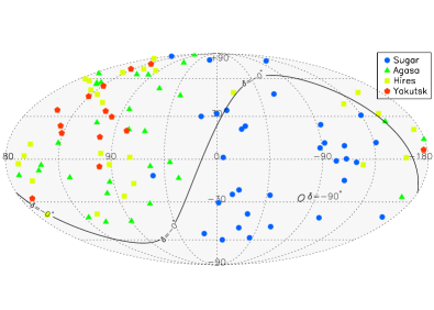
Figure 1: Skymap of the UHECR arrival directions of events in galactic coordinates with rescaled energy $E>4\times 10^{19}$ eV. The solid line is the celestial equator.

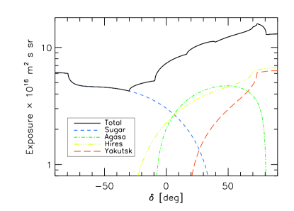
Figure 2: Single and combined exposures for the various experiment considered: Sugar (red), Hires (green), Agasa (blue), Yakutsk (yellow), combined (black).

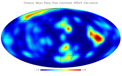
Figure 3: The UHECR flux contrast map (or excess map) properly smoothed with a Gaussian filter of $10^{\circ}$ width.

II.1 The data

In our analysis, we closely follow the approach reported in Kachelriess:2005uf ; Cuoco:2006dx , using a similar dataset extracted from available publications or talks of the AGASA Hayashida:2000zr , Yakutsk yakutsk , SUGAR Winn:1986un , and HiRes collaborations Abbasi:2004ib ; Hires2 . Note that we rescale a priori the energies of the experiments to the HiRes one and consider events above $E\geq 4\times 10^{19}\,$eV in this renormalized sample. This approach is applied hereafter in the analysis and we address the reader to Kachelriess:2005uf for further details. In Fig. 1 we show the points used in this analysis in galactic coordinates, while Fig. 2 reports the single and combined exposure for the various experiments as a function of the declination, in the limit of saturated acceptance and mediated over the right ascension (see e.g. Sommers:2000us ). In Fig. 3 we show the derived UHECR excess map (flux over average expected flux, minus one) properly smoothed by a gaussian filter of $10^{\circ}$. Such a choice for the width amplitude (which has only illustrative purposes) represents an acceptable compromise between the few degrees of the experimental uncertainty on the arrival direction of UHECR, and the typical angular length of the nearby astrophysical structures of several tens of degrees. Of course, the data have been properly weighted by the exposure.

The smoothed map in Fig. 3 clearly shows that the most apparent visual feature in the data is the medium scale clustering, with the data clustered in few spots of $20^{\circ}$-$30^{\circ}$ degrees each, that in their turn are distributed almost uniformly in the sky. This is of course the reason of the signal found in Kachelriess:2005uf with a proper statistical analysis. The clustering seen in the southern hemisphere is due to the Sugar data only and has thus a weak statistical evidence. However, the clustering signal is indeed present and statistically significant also considering the data from the northern hemisphere only Kachelriess:2005uf . Indeed, hints of this clustering in the northern hemisphere were recognized already some years ago Stanev:1995my . Finally, lowering the energy threshold the signature disappears, excluding the possibility that the signal is only a systematic feature coming from an incorrect modeling of the exposures Kachelriess:2005uf .

Concerning possible interpretations of the signal, here we report a few general considerations, while more quantitative analyses are reported in the following. The absence of a correlation with the Galactic Plane or the absence of excess toward the Galactic Center disfavor respectively Galactic astrophysical sources and heavy relic decays in our Galactic Halo as origin of these events. Qualitatively, extragalactic sources of astrophysical nature appear the most likely accelerators. In these scenarios, unless only a handful of sources dominate the emission, the pattern of the arrival directions of the events should reflect to some extent the one of large scale structures in the nearby universe. Actually the degree of clustering observed is quite pronounced. It exceeds also the anisotropy expected in the minimal case of proton primaries (with a GZK horizon $z\simeq 0.06$), which is in marginal agreement with the data (see Cuoco:2006dx and section III). Thus, the few prominent structures visible naturally suggest either a scenario where the UHE sky is dominated by few nearby powerful sources or one where UHECRs are produced by a relatively larger number of sources significantly biased with overdensities in the local universe (within $z\simeq 0.02$). Both scenarios require an important role of magnetic fields, either galactic or extragalactic, to accommodate deflections of the order $\gtrsim$10^∘. In the former case such deflections are necessary to explain the large smearing of the point sources emission and in the latter to justify the lack of a significant correspondence between the data and the nearby galaxy clusters.

II.2 The models

The previous discussion motivates an extension of the previous analysis reported in Cuoco:2006dx along two directions:

• assuming a smaller horizon, i.e. biasing the correlation with LSS towards closer sources;

• studying the impact of the GMF on the autocorrelation signature and on the cross-correlation signal.

Both extensions should be regarded as “first order” refinements of our previous study. The point ($II$) does not need much justification: it is important to establish the robustness of the previous results with respect to the effects of astrophysical magnetic fields. Even if extragalactic magnetic fields may have a major role in shaping or preserving the UHECR anisotropies, very little is known about them (see Dolag:2003ra and ems ). On the other hand we know for sure that a regular GMF exists—although we have only rough ideas on its magnitude and structure—and it is in principle relevant for UHECR deflections, even in the case of pure proton composition. In the following, we shall then consider how our results change when data are corrected for the effects of a few GMF models available in the literature. In particular, we shall use the three models HMR, TT, and PS employed in Kachelriess:2005qm , which we refer to for details. To account for the deflections in the GMF in our analyses we shall follow the back-tracking technique described in Takami:2005ij ; Harari:1999it . The technique consists in mapping the arrival CRs directions on the Earth backward outside the GMF to obtain a map of the GMF deflections. We then apply the mapping to the extragalactic expected CR map and correct it for the GMF displacements. The extragalactic CRs map $F({E_{\rm{cut}}},\hat{\Omega})$ expected at an energy greater than $E_{\rm{cut}}$ at the direction $\hat{\Omega}$ is obtained as described in Cuoco:2005yd . The map is then convolved with the GMF deflections to have $F({E_{\rm{cut}}},\hat{\Omega}(\hat{\Omega}^{\prime}))$ where $\hat{\Omega}(\hat{\Omega}^{\prime})$ is the mapping produced by the back-tracking technique. This method is fully suited for the cases in which energy losses along the particle track are negligible and when the particle energy is large enough to exclude loops and/or trapped regions during the propagation. Both these conditions are satisfied for the UHECRs and for the GMFs we considered. Also note that an isotropic sky remains isotropic under the GMF transformation, in agreement with the expectation from the Liouville theorem. We refer to Kachelriess:2005qm ; Takami:2005ij ; Harari:1999it for details.

For simplicity we only consider the mapping produced for a fixed rigidity corresponding to the energy $E_{\rm{cut}}$ (with the choice $E_{\rm{cut}}$=40 EeV in the present case). This should be a reasonable approximation, equivalent to replace the steep ($\propto E^{-3}$) UHECRs spectrum above $E_{\rm{cut}}$ with a delta-function at $E_{\rm{cut}}$. Beside the steepness of the UHECR spectrum, a further motivation for this approximation is that we are not considering the shift of single objects but of an overall map, already smoothed at a scale of order $\sim 5^{\circ}$ (we are not interested to the very small scales, indeed). Finally, we shall show in the next section that the auto-correlation analysis is quite insensitive to the details of the GMFs or the assumed rigidity as long as the magnetic deflections effects remains moderate, so that the approximation is also justified a posteriori, at least for autocorrelations studies. The effects are potentially larger for cross-correlation analyses, which however are already less robust for other reasons.

A further possible problem is given by the fact that the mask region present in the catalogue and excluded from the analysis is distorted by the effect of the GMF, so that in principle one should exclude, case by case, the regions which the mask is mapped into by the GMF. We neglect this effect assuming the the mask is approximately mapped in itself by the GMF transformation. This is a quite good approximation for the region near the galactic plane while it is not satisfied by the two narrow stripes. However, the the stripes amount to about 10% of the total mask and only roughly 2% of the whole sky, which is a very small bias for our purposes in this work.

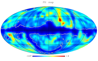
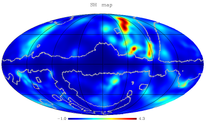
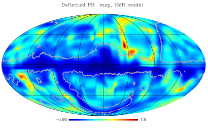
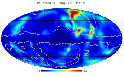
Figure 4: Top row: Excess maps of PH (left) and SH models (right) in galactic coordinates. The grey contour bounds the blind region of PSCz catalogue. Bottom row: Galactic excess maps of the PH (left) and SH models (rigth) taking into account the Galactic magnetic field correction for a specific model (HMR in Kachelriess:2005qm ) and assuming proton primaries ($Z=1$).

From a qualitative point of view, the point ($I$) is reasonable, too. In many scenarios, only relatively nearby sources (if any) may be identifiable in cosmic ray maps. There are several plausible reasons for that. Even in absence of magnetic fields, an heavier composition implies a different energy-loss horizon for UHECRs Harari:2006uy ; Hooper:2006tn . For the energy threshold considered here ($E\gtrsim 4\times 10^{19}\,$eV), this is smaller than the proton one. In presence of extragalactic magnetic fields, the propagation of a UHECR may greatly differ from a straight line and in principle may even happen in a diffusive regime Sigl:1998dd ; Lemoine:1999ys ; Deligny:2003rp ; Parizot:2004wh . Although it is unlikely that the propagation is truly diffusive, Gpc-scale pathlengths for protons injected within a few hundreds Mpc may be common even above 10 EeV Armengaud:2004yt . A non-negligible role of magnetic fields would have two consequences: for a given energy-loss mechanism, it is clear that the true horizon may be significantly shorter than the expected one. Thus, UHECRs above a given $E_{\rm th}$ may be largely collected within a region smaller than the linear energy-loss horizon. More important, apart for energy losses, the longer the propagation time, the smaller the chance that intrinsic anisotropies may survive (in some form). Finally, since UHECR source likely have to meet special accelerator requirements, it is reasonable to conceive a relatively rare population of sources, possibly strongly biased with respect to LSS.

However, how to implement in practice point $(I)$ is admittedly not model independent. One possibility may be to cut arbitrarily a LSS catalogue to some redshift $z_{\rm cut}$, and consider only correlations with structures within this distance, assuming for the rest that UHECRs are unbiased tracers of LSS (i.e. neglecting otherwise energy loss effects). Another possibility is to create anisotropy map templates of specific scenarios for UHECR composition, sources, and extragalactic magnetic fields, comparing them with the observed configurations of data in order to infer the best model. Although this will be the way to proceed when high statistics will be achieved, at the moment it could just dilute the basic consequence of our assumption ($I$) under a large number of unknown parameters. To keep some physical-inspired input in a toy model, we shall compare the distribution of data as in Fig. 1 with the LSS maps obtained by convolution of the PSCz catalogue with an energy-loss window function corresponding to protons twice more energetic, i.e. $E=8\times 10^{19}\,$eV, implying an effective horizon $z\simeq 0.02$ Cuoco:2005yd . We shall denote this scenario as “small horizon” (SH), as opposed to the “proton horizon” (PH) as treated in Cuoco:2006dx and corresponding to the minimal assumption of protons primaries with $E\geq 4\times 10^{19}\,$eV propagating in a negligible EGMF (usual GZK horizon $z\simeq 0.06$). In the top two panels of Fig. 4 we report the PH and SH maps. The smoothing is variable and it is related to the adaptive smoothing applied to the PSCz catalogue to minimize the effect of the shot noise. We emphasize that this should be considered a toy model, and not a realistic scenario for UHECR sources or composition. However, our toy model may be indicative of a plausible situation where at least for anisotropy searches the useful UHECR horizon is relatively short.

II.3 Statistical tools

For the statistical analysis we define the (cumulative) autocorrelation function $w$ as a function of the separation angle $\delta$ as

$$w(\delta)=\sum_{i=2}^{N_{d}}\sum_{j=1}^{i-1}\Theta(\delta-\delta_{ij}),$$ (1)

where $\Theta$ is the step function, $N_{d}$ the number of CRs considered and $\delta_{ij}=\arccos(\cos\rho_{i}\cos\rho_{j}+\sin\rho_{i}\sin\rho_{j}\cos(\phi_{i}-\phi_{j}))$ is the angular distance between the two cosmic rays $i$ and $j$ with coordinates $(\rho,\phi)$ on the sphere. Analogously, one can define the correlation function $\xi(\delta)$ as

$$\xi(\delta)=\sum_{i=1}^{N_{d}}\sum_{a=1}^{N_{s}}\Theta(\delta-\delta_{ia})\,,$$ (2)

where $\delta_{ia}$ is the angular distance between the CR $i$ and the candidate source $a$ and $N_{s}$ is the number of source objects considered.

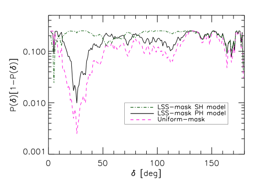
Figure 5: Chance probability of auto correlation taking as reference model an uniform distribution, the linear correlation model of Cuoco:2006dx (LSS-PH model) and the presently considered model with a smaller horizon (LSS-SH model).

We perform a large number $M\simeq 10^{5}$ of Monte Carlo simulations of $N$ data sampled from a distribution on the sky corresponding to the hypothesis $H$ (e.g., uniform, LSS, etc.) and for each realization $j$ we calculate the autocorrelation function $w_{j}^{H}(\delta)$. The sets of random data match the number of data for the different experiments passing the cuts after rescaling, and are spatially distributed according to the exposures of the experiments. The formal probability $P^{H}(\delta)$ to observe an equal or larger value of the autocorrelation function by chance is

$$P^{H}(\delta)=\frac{1}{M}\sum_{j=1}^{M}\Theta[w_{j}^{H}(\delta)-w_{\star}(\delta)],$$ (3)

where $w_{\star}(\delta)$ is the observed value for the cosmic ray dataset and the convention $\Theta(0)=1$ is being used. Relatively high values of $P$ and $1-P$ indicate that the data are consistent with the null hypothesis being used to generate the comparison samples, while low values of $P$ or $1-P$ indicate that the model is inappropriate to explain the data. That is, in the following we shall plot the function $P(\delta)\times[1-P(\delta)]$, which vanishes if any of $P$ or $1-P$ vanishes and has the theoretical maximum value of $1/4$. Thus, the higher its value is the more consistent the data are with the underlying hypothesis. Note also that by construction the values at different $\delta$ of the function $P(\delta)$ are not independent.

To calculate the cross-correlation probability, we perform a large number $M(\simeq 10^{5})$ Monte Carlo realization of $N$ events is sampled according to the LSS probability distribution, and for each realization $i$ we calculate the function $\xi_{i}^{\rm LSS}(\delta)$. We generate analogously $M$ random datasets from an uniform distribution, and calculate $\xi_{j}^{\rm uni}(\delta)$. We have thus $M^{2}$ independent couples of functions $(i,j)$. The fraction of the $M^{2}$ simulations where the condition $\xi^{\rm uni}(\delta)\geq\xi^{\rm LSS}(\delta)$ is fulfilled is the probability

$$P_{\xi}(\delta)=\frac{1}{M^{2}}\sum_{i=1}^{M}\sum_{j=1}^{M}\Theta[\xi_{i}^{\rm uni}(\delta)-\xi_{j}^{\rm LSS}(\delta)]\,.$$ (4)

A technical detail of the analysis is related to the presence of the catalogue mask. This includes a zone centered on the galactic plane and caused by the galactic extinction and a few, narrow stripes which were not observed with enough sensitivity by the IRAS satellite. These regions are excluded from our analysis with the use of the binary mask available with the PSCz catalogue itself. This reduces the available sample by about 10%.

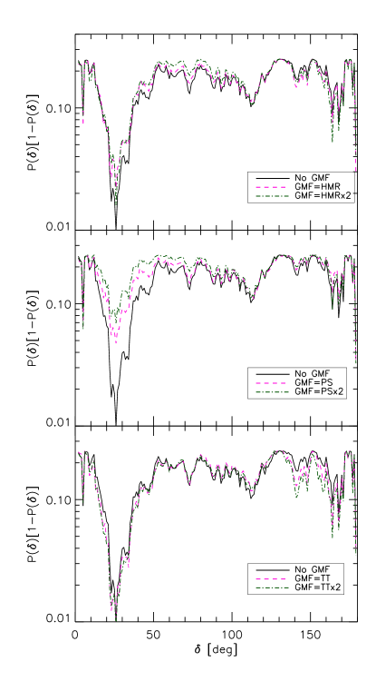
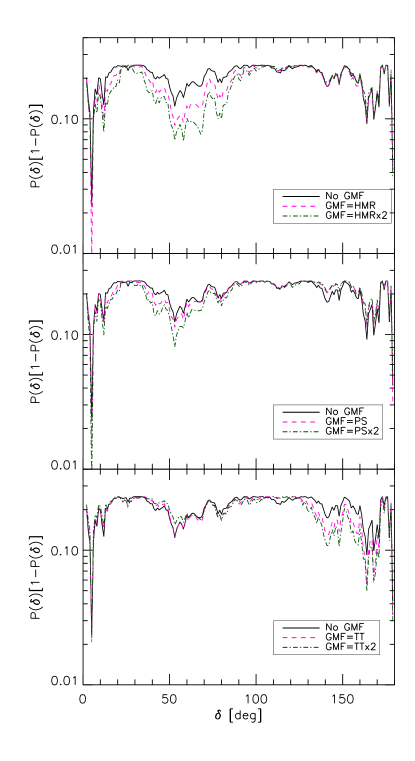
Figure 6: Chance probability of autocorrelation of the data for different GMF models and for the PH model maps (left) and SH model maps (right) taken as reference sample. The cases $Z=1$ and $Z=2$ are shown in each panel.

III Results

By repeating our analysis in Cuoco:2006dx following the SH model and without considering for the moment the effects of the GMF, we obtain the results shown in Fig. 5. The SH model seems to explain extremely well the clustering properties of the data, with the related $P\times(1-P)$ curve almost coincident with the ideal $P=0.5$ expectation. Not surprisingly, this can be understood after a visual inspection of the maps in Fig. 3 (data) and Fig. 4 (models). While the map from protons with $E\geq 4\times 10^{19}\,$eV (the PH model) is still too much isotropic with respect to the data, in the SH map the number of clusters and their distribution resemble much more the data, in that it leaves typical “voids” between clustered hot-spots observed.

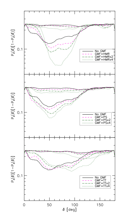
Figure 7: Cross-correlation chance probability between the different LSS models and the data, with the solid lines representing the result uncorrected for the GMF. Upper set of curves in each panel refer to the PH model while lower ones to the SH model.

Our next step is to investigate the effects of the galactic magnetic field. In the two bottom panels of Fig. 4 we show the effective modification of LSS structures happening for the PH and the SH scenario, assuming as example the HMR model in Kachelriess:2005qm . In general, besides the shifting of the positions of the structures, as expected the GMF introduces in the deflected maps also other peculiar lensing phenomena like shearing and (de)magnification Harari:1999it . More quantitatively, the effects of the GMF are studied in the following through the modifications induced in the auto and cross-correlation functions. In Fig. 6 we investigate the effect of the GMF on the signature in the autocorrelation function. We also show the effect of changing the rigidity of the particles. Actually, the equations of motion for CRs in the GMF only depend on the parameter $C=B\times Z/E$ where $B,Z,E$ are respectively the GMF normalization, the particle atomic number (electric charge of the nucleus) and the particle energy. A combination of parameters that leaves unchanged $C$ is thus completely degenerate from the point of view of propagation in the GMF (though, of course, not for the energy losses in the propagation in the extragalactic sky.) As a general consideration, we see that at least for the baseline cases considered, the correction for the GMF does not destroy the pattern in $P(1-P)$, but can improve or worsen it at most by a factor of a few. On the other hand, extreme changes in $C$ may significantly alter the pattern of the function.

Finally, in Fig. 7 we report the results of the cross correlation analysis. Note that, while in the previous case we were repeating the same test of Ref. Kachelriess:2005uf , here we perform a different test, and to assess the confidence level of any statistically significant signal we might find one should carefully evaluate the penalty factor. Unfortunately, in no case we find a statistically significant signal (namely, not even at the nominal level). Yet, qualitatively all the SH maps show some improvement with a nominal $P_{\xi}\sim 10\%$ (with respect to $P_{\xi}\sim 50\%$ for the PH case), even without use of the GMF correction. This is understood since we have about the same number of clusters in the data and in the map and typically one can find a correspondence between the two within a radius of roughly $50^{\circ}$. A more significant signal of cross-correlation should eventually peak within $\sim 25^{\circ}$ (the typical size of the clusters) signaling a superposition of the data and map clusters. Once again, no significant difference arises when the data are corrected for the GMF. Although the minimum of the probability can change by up to a factor of a few, it does not move towards $\delta\simeq 0^{\circ}$, as it should be if the GMF were correctly shifting the hot-spots.

An important point to stress is that while an evidence of cross-correlation would be tantalizing signature of a discovery, the lack of it can not be easily used as an argument against the hypothesis. The cross-correlation signal is indeed much more sensitive than the autocorrelation one to magnetic fields deflection and, importantly, to unknown experimental systematic effects. For the case at hand, the main responsables of the displacement up to 50 degrees between clusters in the data and overdensities in the LSS are the hot-spots from the SUGAR data, which is the experiment among the ones considered which mostly suffers for a poor angular resolution, beside not well-understood systematics in the energy scale determination. Indeed, limiting the analysis to the northern hemisphere experiments only, the data show quite a good cross-correlation with the local over-density of matter, especially within $z\sim$ 0.02. More noticeably, they fall relatively close to the so-called Super-Galactic plane, as can be appreciated also from a comparison between Fig. 1 and Fig. 4. This correspondence was already noticed by the authors of ref. Stanev:1995my and further assessed in ref. Burgett:2003yg . So, while the features in the cross-correlation function vary quite a bit excluding e.g. one dataset, the auto-correlation ones do not, as discussed more extensively in Kachelriess:2005uf .

Aware of this caveat, it is still worth exploring the consequences of assuming that displacements up to 50^∘ with respect to the true sources are effective. Under this hypothesis, and, if the signal corresponds to extragalactic structures, we would be brought to conclude that: (i) if UHECRs are dominated by protons, then there are significant deflections by extragalactic magnetic fields. Indeed, although the GMF may be not well reproduced by current models, even changing within reasonable ranges the GMF geometry and intensity no appreciable cross-correlation at small angles appears. (ii) If there is a significant fraction of heavy nuclei in the UHECR flux, results may be also explained with a negligible role of extragalactic magnetic fields, attributing to GMF deflections the significant ($\sim 30^{\circ}$–$50^{\circ}$) displacement between the observed clusters in the data and the real galaxy clusters. Note that, if in any case overall deflections as large as $\sim 50^{\circ}$ are effective, peculiar manifestations of regular deflections in the magnetic field—like elongations directed towards structures with a proper ordering of energies—may not be observable due to non-negligible non-linearities, especially in the case of a chemically inhomogeneous sample of UHECRs. Yet, if this interpretation would turn out to be the correct one, we expect that once higher statistics will be available at higher energies, these features will eventually show up in the data, a prediction that can eventually be confirmed by Auger.

IV Discussion and Conclusion

The anisotropy pattern of the combined UHECRs data (re-scaled energy $E=4\times 10^{19}\,$eV in HiRes scale), although compatible with isotropy at very large angular scales, shows a peculiar medium scale clustering corresponding to 6-7 spots of roughly $20^{\circ}$-$30^{\circ}$ degrees of extension distributed uniformly in the sky. If confirmed, this would have a wealth of consequences for the long-awaited astronomy of UHECRs. At a general level, the absence of a correlation with the Galactic Plane or the absence of an excess toward the Galactic Center disfavor respectively Galactic astrophysical sources and heavy relic decays in our Galactic Halo as origin of these events. Extragalactic sources of astrophysical nature appear instead the most likely accelerators consistent with these features. Should forthcoming data show similar features, the first realistic quantities one could extract from the clustering are constrains the number density of the sources as well as their type, from their bias with respect to LSS (see Cuoco:2007id and references therein). As next goal, one should be able to establish explicit cross-correlation with extragalactic structures and/or hints in that direction, as elongations of events directed toward the sources, whose distance should scale inversely to the UHECR energy. More “conventional” astronomy, determining the locations of single UHECR sources and perhaps of their spectrum is likely demanded to a subsequent phase when sufficient statistics will be available.

Although the clustering properties in the data are intriguing, the interpretation of the signature is puzzling, especially in absence of a significant statistics at higher energy and of chemical composition constraints. The comparison between significant sets of data at different energy cuts may reveal the importance of magnetic deflection effects. At the moment, we can only speculate on the possible implications of the signal—assuming it is not a statistical fluke—under some simplifying hypotheses.

One possibility is that these excesses may trace LSS overdensities in the near universe (within the GZK-sphere). The autocorrelation analyses reported in this paper show that this interpretation is indeed favored in particular if the effective horizon is smaller than the GZK one for protons of the assumed energy. Both a significant fraction of heavier nuclei and a significant role of extragalatic magnetic fields may cause this effect (the former might be favored by recent Auger data Unger:2007mc .) Although not statistically significant, this interpretation may be supported by a weak hint of a broad minimum in the cross correlation function (at the level of nominal chance probability of 10%-15%) around 50^∘ if a small horizon ($z\lesssim 0.02$) is assumed. Both signatures are relatively robust with respect to deflections in typical GMF models, although some marginal improvement or worsening may arise for some choices of the GMF model and effective rigidities. In this case, the size of the hot-spots would be due partly to the one of the largest overdensities in the local LSS and partly to magnetic smearing needed to explain the overall deflection with respect to the LSS. The latter effect would be in general subleading but for the SUGAR hotspots in the Southern Emisphere, which are the most distant ones from overdensities. This may be physically associated to the more intense magnetic fields towards the central regions of our Galaxy to which SUGAR is pointing. An alternative interpretation of the data is that they are due to very few ($\cal{O}$(5-6)) powerful sources. Yet, the smearing of a point-like emission to the level of the observed spots of $\cal{O}$(20^∘) would require a quite extreme magnetized environment Sigl:1998dd ; Lemoine:1999ys .

In any case, the hints for some structures in the data are very exciting, and we urge an independent cross-check with the nowadays large statistics collected by Auger. If confirmed, together with the indication for the presence of a GZK-like feature in the energy spectrum of HiRes data Abbasi:2007sv , this likely implies that UHECR are dominated by astrophysical sources (as opposed to exotic scenarios). However, far from being the end of the UHECR saga, the combined use of spectral information, chemical composition constraints, and anisotropy maps at different energies would offer the tools for the long-awaited hunt for the UHECR accelerators.

References

- (1) K. Greisen, “End To The Cosmic Ray Spectrum?,” Phys. Rev. Lett. 16, 748 (1966).
- (2) G. T. Zatsepin and V. A. Kuzmin, “Upper Limit Of The Spectrum Of Cosmic Rays,” JETP Lett. 4, 78 (1966) [Pisma Zh. Eksp. Teor. Fiz. 4, 114 (1966)].
- (3) R. Abbasi et al. [HiRes Collaboration], “Observation of the GZK cutoff by the HiRes experiment,” astro-ph/0703099.
- (4) A. Cuoco, R. D. Abrusco, G. Longo, G. Miele and P. D. Serpico, “The footprint of large scale cosmic structure on the ultra-high energy cosmic ray distribution,” JCAP 0601 (2006) 009 [astro-ph/0510765].
- (5) Pierre Auger Collaboration, 1996 The Pierre Auger Project Design Report, FERMILAB-PUB-96-024.
- (6) Abraham J et al. (Pierre Auger Collaboration), “Properties and performance of the prototype instrument for the Pierre Auger Observatory,” 2004 Nucl. Instrum. Meth. A 523 50.
- (7) L. A. Anchordoqui, C. Hojvat, T. P. McCauley, T. C. Paul, S. Reucroft, J. D. Swain and A. Widom, “Full-sky search for ultrahigh-energy cosmic ray anisotropies,” Phys. Rev. D 68 (2003) 083004 [astro-ph/0305158].
- (8) M. Kachelrieß and D. V. Semikoz, “Clustering of ultra-high energy cosmic ray arrival directions on medium scales,” Astropart. Phys. 26 (2006) 10 [astro-ph/0512498].
- (9) M. Takeda et al., “Small-scale anisotropy of cosmic rays above 10**19-eV observed with the Akeno Giant Air Shower Array,” Astrophys. J. 522, 225 (1999) [astro-ph/9902239].
- (10) P. G. Tinyakov and I. I. Tkachev, “Correlation function of ultra-high energy cosmic rays favors point sources,” JETP Lett. 74, 1 (2001) [Pisma Zh. Eksp. Teor. Fiz. 74, 3 (2001)] [astro-ph/0102101].
- (11) C. B. Finley and S. Westerhoff, “On the evidence for clustering in the arrival directions of AGASA’s ultrahigh energy cosmic rays,” Astropart. Phys. 21, 359 (2004) [astro-ph/0309159].
- (12) S. Mollerach [Pierre Auger Collaboration], “Studies of clustering in the arrival directions of cosmic rays detected at the Pierre Auger Observatory above 10 EeV,” arXiv:0706.1749 [astro-ph].
- (13) A. Cuoco, G. Miele and P. D. Serpico, “First hints of large scale structures in the ultra-high energy sky?,” Phys. Rev. D 74 (2006) 123008 [astro-ph/0610374].
- (14) W. Saunders et al., “The PSCz Catalogue,” Mon. Not. Roy. Astron. Soc. 317, 55 (2000). [astro-ph/0001117].
- (15) N. Hayashida et al., “Updated AGASA event list above 41019 eV,” astro-ph/0008102.
-
(16)
Talk of M. Pravdin at the 29th ICRC Pune 2005,
http://icrc2005.tifr.res.in/htm/PAPERS/HE14/ rus-pravdin-MI-abs1-he14-poster.pdf - (17) M. M. Winn et al., “The cosmic ray energy spectrum above 1017 eV,” J. Phys. G 12 (1986) 653.
- (18) R. U. Abbasi et al. [The High Resolution Fly’s Eye Collaboration (HIRES)], “Study of small-scale anisotropy of ultrahigh energy cosmic rays observed in stereo by HiRes,” Astrophys. J. 610, L73 (2004). [astro-ph/0404137].
-
(19)
Talk of S. Westerhoff at the CRIS-2004 workshop “GZK and
Surrounding”, Catania, Italy,
http://www.ct.infn.it/cris2004/talk/westerhoff.pdf, also in Nucl. Phys. Proc. Suppl. 136C (2004) 46 [astro-ph/0408343]. - (20) P. Sommers, “Cosmic Ray Anisotropy Analysis with a Full-Sky Observatory,” Astropart. Phys. 14, 271 (2001) [astro-ph/0004016].
- (21) T. Stanev, P. L. Biermann, J. Lloyd-Evans, J. P. Rachen and A. Watson, “The Arrival directions of the most energetic cosmic rays,” Phys. Rev. Lett. 75 (1995) 3056 [astro-ph/9505093]; See also the study by G. A. Medina-Tanco, “Large scale distribution of matter in the nearby universe and ultra-high energy cosmic rays,” astro-ph/9707054.
- (22) K. Dolag, D. Grasso, V. Springel and I. Tkachev, “Mapping deflections of Ultra-High Energy Cosmic Rays in Constrained Simulations of Extragalactic Magnetic Fields,” JETP Lett. 79, 583 (2004) [Pisma Zh. Eksp. Teor. Fiz. 79, 719 (2004)] [astro-ph/0310902]; See also “Constrained simulations of the magnetic field in the local universe and the propagation of UHECRs,” astro-ph/0410419.
- (23) G. Sigl, F. Miniati and T. Enßlin, “Ultra-High Energy Cosmic Ray Probes of Large Scale Structure and Magnetic Fields” Phys. Rev. D 70, 043007 (2004) [astro-ph/0401084]; see also “Cosmic magnetic fields and their influence on ultra-high energy cosmic ray propagation,” Nucl. Phys. Proc. Suppl. 136 (2004) 224, astro-ph/0409098.
- (24) M. Kachelriess, P. D. Serpico and M. Teshima, “The galactic magnetic field as spectrograph for ultra-high energy cosmic rays,” Astropart. Phys. 26, 378 (2006) [astro-ph/0510444].
- (25) H. Takami, H. Yoshiguchi and K. Sato, “Propagation of ultra-high energy cosmic rays above 10**19-eV in a structured extragalactic magnetic field and galactic magnetic field,” Astrophys. J. 639, 803 (2006) [Erratum-ibid. 653, 1584 (2006)] [astro-ph/0506203].
- (26) D. Harari, S. Mollerach and E. Roulet, “The toes of the ultra high energy cosmic ray spectrum,” JHEP 9908 (1999) 022, astro-ph/9906309.
- (27) D. Harari, S. Mollerach and E. Roulet, “On the ultra-high energy cosmic ray horizon,” JCAP 0611 (2006) 012 [astro-ph/0609294].
- (28) D. Hooper, S. Sarkar and A. M. Taylor, “The intergalactic propagation of ultra-high energy cosmic ray nuclei,” Astropart. Phys. 27 (2007) 199 [astro-ph/0608085].
- (29) G. Sigl, M. Lemoine and P. Biermann, “Ultra-high energy cosmic ray propagation in the local supercluster,” Astropart. Phys. 10, 141 (1999) [astro-ph/9806283].
- (30) M. Lemoine, G. Sigl and P. Biermann, “Supercluster Magnetic Fields and Anisotropy of Cosmic Rays above 1019 eV,” arXiv:astro-ph/9903124.
- (31) O. Deligny, A. Letessier-Selvon and E. Parizot, “Magnetic Horizons Of Uhecr Sources And The Gzk Feature,” Astropart. Phys. 21 (2004) 609 [astro-ph/0303624].
- (32) E. Parizot, “GZK horizon and magnetic fields,” Nucl. Phys. Proc. Suppl. 136 (2004) 169 [astro-ph/0409191].
- (33) E. Armengaud, G. Sigl and F. Miniati, “Ultrahigh energy nuclei propagation in a structured, magnetized universe,” Phys. Rev. D 72, 043009 (2005) [astro-ph/0412525].
- (34) W. S. Burgett and M. R. O’Malley, “Hints of energy dependences in AGASA EHECR arrival directions,” Phys. Rev. D 67 (2003) 092002 [arXiv:hep-ph/0301001].
- (35) A. Cuoco, S. Hannestad, T. Haugboelle, M. Kachelriess and P. D. Serpico, “Clustering properties of ultrahigh energy cosmic rays and the search for their astrophysical sources,” arXiv:0709.2712 [astro-ph].
- (36) M. Unger [Pierre Auger Collaboration], “Study of the Cosmic Ray Composition above 0.4 EeV using the Longitudinal Profiles of Showers observed at the Pierre Auger Observatory,” arXiv:0706.1495 [astro-ph].
- (37) K. M. Gorski, E. Hivon, A. J. Banday, B. D. Wandelt, F. K. Hansen, M. Reinecke and M. Bartelman, “HEALPix – a Framework for High Resolution Discretization, and Fast Analysis of Data Distributed on the Sphere,” Astrophys. J. 622 (2005) 759 [astro-ph/0409513].