Keldysh Ginzburg-Landau action of fluctuating superconductors

Abstract

We derive Ginzburg-Landau action by systematically integrating out electronic degrees of freedom in the framework of the Keldysh nonlinear $\sigma$-model of disordered superconductors. The resulting Ginzburg-Landau functional contains a nonlocal $\Delta$-dependent contribution to the diffusion constant, which leads, for example, to Maki-Thompson corrections. It also exhibits an anomalous Gor’kov-Eliashberg coupling between $\Delta$ and the scalar potential, as well as a peculiar nonlocal nonlinear term. The action is gauge invariant and satisfies the fluctuation dissipation theorem. It may be employed, e.g., for calculation of higher moments of the current fluctuations.

I Introduction

Time dependent Ginzburg-Landau (TDGL) theory has received a lot of attention and was a subject of controversy over many years. Schmid ; Abrahams ; Caroli-Maki ; Gorkov-Eliashberg ; Woo-Abrahams ; Eliashberg ; Houghton-Maki ; Hu-Thompson ; Cyrot ; Kramer ; Schon ; Hu ; Watts-Tobin ; Krempasky ; Otterlo Gor’kov and Eliashberg Gorkov-Eliashberg (GE) were probably among the first who realized that the thermodynamic Ginzburg-Landau equation may be generalized for the time-dependent phenomena in the case of gapless superconductivity (see also earlier publications Schmid ; Caroli-Maki ). The latter occurs either in the presence of magnetic impurities, or in the fluctuating regime at $T>T_{c}$. Notably GE equation contained an anomalous nonlocal coupling between the order parameter $\Delta$ and the scalar potential: the fact that was frequently overlooked in many subsequent treatments.

Extension of the TDGL theory to a gapped phase turns out to be a very demanding problem. As noted by Gor’kov and Eliashberg, the difficulty stems from the singularity of the BCS density of states at the gap edge. The latter leads to a slowly decaying oscillatory response at frequency $2\Delta/\hbar$ in the time domain. As a result, the expansion in powers of the small parameter $\Delta/T_{c}$ fails. In principle, it may be augmented by an expansion in $\Delta/(\hbar\omega)$, in case the external fields are high-frequency ones. To describe low-frequency responses in the gapped phase, one needs a time nonlocal version of the TDGL theory. The analysis is greatly simplified in the presence of a pair-breaking mechanism, such as magnetic impurities or energy relaxation. Such a mechanism may eliminate singularity in the density of states, leading to gapless phase in the presence of finite $\Delta$. Under these conditions, an expansion in powers of $\Delta\tau_{\phi}/\hbar$ and $\omega\tau_{\phi}$ is justified and thus a time-local TDGL equation may be derived (here $\tau_{\phi}$ is the pair-breaking time). In the present work, we restrict ourselves to the fluctuating regime $T>T_{c}$, where the spectrum is gapless automatically and there is no need in an explicit pair-breaking mechanism.

Soon after the GE work, Aslamazov-Larkin (AL) Aslamazov-Larkin and Maki-Thompson (MT) Maki ; Thompson corrections to conductivity of fluctuating superconductors were discovered in the diagrammatic linear response framework. While AL term had naturally followed from TDGL theory (see, e.g., books Abrikosov ; Tinkham ; Larkin-Varlamov ), MT phenomena were seemingly absent in TDGL formalism. Based on the work, Houghton-Maki it was proposed Cyrot that in order to include MT term into the set of TDGL equations, one has to substitute the renormalized conductivity $\sigma\rightarrow\sigma+\sigma^{MT}$ in the expression for the current, supplementing TDGL equation. While leading to the correct static average current (by construction), this way of handling the problem fails to satisfy the fluctuation-dissipation theorem (FDT). Indeed, it does not provide any prescription for calculating higher moments of the current (even in equilibrium). Another drawback of the approach of Ref. [Cyrot, ] is that it fails to incorporate a peculiar frequency dependence of MT phenomena, stemming from the time nonlocality of MT terms. The procedure introduced phenomenologically in Ref. [Cyrot, ] was latter elegantly derived in Ref. [Volkov-Nagaev, ] using nonequilibrium Green functions technique. Let us also mention few other works where a combined set of TDGL and kinetic equations was suggested.Krempasky ; Hu An imaginary-time action of fluctuating superconductors was discussed in Ref. [Otterlo, ].

In the present publication, we derive a set of coupled stochastic TDGL and Maxwell equations, which are suitable for calculation of both average current and its higher moments. This set of equations is an immediate consequence of the effective Keldysh action written in terms of the fluctuating order parameter and electromagnetic potentials. Technically, we employ the nonlinear $\sigma$-model in the Keldysh representation KA ; FLS to perform disorder averaging. We then systematically integrate out the electronic degrees of freedom, neglecting Anderson localization effects. The resulting effective action, written in terms of the order parameter and electromagnetic potentials, naturally and unmistakably contains both MT terms and anomalous GE coupling between the order parameter and electric field.

We restrict ourselves with the fluctuating regime $T>T_{c}$ only, leaving the case $T<T_{c}$ (and magnetic impurities) for future studies. As always, the Ginzburg-Landau treatment requires the condition

$$T-T_{c}\ll T_{c}\,,$$ (1)

which is central to our consideration. We also assume that both the order parameter and the electromagnetic fields vary on the spatial scale which is much larger than $\xi_{0}=\sqrt{D/T_{c}}$ (here $D$ is the diffusion constant) and the time scale which is much slower than $1/T_{c}$ (hereafter we adopt units, where $\hbar=c=1$). Moreover, we shall rely on the fact that the electronic system is always in a local thermal equilibrium. This in turn implies that the external fields are not too large. More precisely, the electric field $\bf E$ is such that $eE\xi_{0}\ll T_{c}$, while the magnetic field $\bf H$ is restricted by the condition $eH\xi_{0}\ll 1/\xi_{0}$. Notice that these conditions do not restrict our treatment to the linear response regime. Nonlinear phenomena may be included, as long as a characteristic scale of nonlinear effects satisfies the inequalities given above.

The restrictions on spatial and temporal scales of the external fields along with the fact that electrons are in local equilibrium considerably simplify the theory. In particular, most of the terms in the effective action acquire a local form in space and time. Nevertheless, the effective theory does not take a completely local form. The diffusion constant obtains a $\Delta$-dependent contribution, with essentially nonlocal coupling to the order parameter. If averaged over the fluctuations of the order parameter, this nonlocal term yields MT correction to conductivity. We note, however, that an average current is not the only manifestation of the nonlocal term. The latter also contributes to the current noise as well as to its higher moments. Another nonlocal effect in the effective action is the way the order parameter interacts with the time-dependent electric field. This is the anomalous GE term. There is one special gauge ($\mathcal{K}$-gauge), where an anomalous term takes an especially simple form. In what follows, we shall explain the $\mathcal{K}$-gauge and perform all the calculations in it. The resulting action may be then transformed back into an arbitrary gauge.

The use of the Keldysh formalism is important in several respects. First, it allows to augment the replica trick to perform the quenched disorder averaging procedure. Second and more important, it is the only consistent way to derive real-time dynamics. The use of the imaginary-time formalism, although possible, requires performing the analytical continuation procedure. The latter is known to be exceedingly demanding for MT as well as time nonlocal nonlinear terms. Working directly in real time allows to make all the expressions physically transparent, unobscured by the peculiarities of the analytical continuation. Finally, the Keldysh formalism naturally allows to extend the treatment to the situations, where the assumption of local equilibrium is not applicable. Although not considered in the present work, a treatment of a nonequilibrium fluctuating superconductivity is a subject of great interest.

The rest of the paper is organized as follows. In the next section, we present our main results in the form of the set of coupled stochastic equations for the order parameter and electromagnetic potentials. In Sec. III we introduce the basic elements of the Keldysh nonlinear $\sigma$-model and explain the way the effective action is derived by integrating out diffuson and Cooperon degrees of freedom. Technical details of this procedure are delegated to a number of appendixes. Finally, in Sec. IV, we summarize our findings and briefly discuss their possible applications.

II Set of stochastic equations

The most compact way to present our results is in the form of the effective Keldysh action which is a functional of the fluctuating order parameter and electromagnetic potentials. Since it requires introducing some notations, we postpone discussion of the action until Sec. III. Here, we present an equivalent way to display the same information using the set of stochastic TDGL and Maxwell equations.

In presence of the scalar $\Phi(\mathbf{r},t)$ and vector $\mathbf{A}(\mathbf{r},t)$ potentials the complex order parameter $\Delta(\mathbf{r},t)$ obeys the following TDGL equation:

$$\big{(}\partial_{t}-2ie\,\partial_{t}\mathcal{K}\big{)}\Delta=\left[D\left(\nabla-2ie\mathbf{A}\right)^{2}-\tau^{-1}_{GL}\right]\Delta+\xi_{\Delta}\,,$$ (2)

here $D$ is the diffusion constant, $e$ is the electron charge, and

$$\tau_{GL}=\frac{\pi}{8(T-T_{c})}\,$$ (3)

is the Ginzburg–Landau relaxation time. The field $\mathcal{K}(\mathbf{r},t)$ satisfy the following equation:

$$\left(\partial_{t}-D\nabla^{2}\right)\mathcal{K}(\mathbf{r},t)=\Phi(\mathbf{r},t)-D\,\mbox{div}\mathbf{A}(\mathbf{r},t)\,.$$ (4)

The complex Gaussian noise $\xi_{\Delta}(\mathbf{r},t)$ has the correlator

$$\big{\langle}\xi_{\Delta}(\mathbf{r},t)\,\xi^{*}_{\Delta}(\mathbf{r^{\prime}},t^{\prime})\big{\rangle}={16\,T^{\,2}\over\pi\nu}\,\,\delta_{\mathbf{r}-\mathbf{r^{\prime}}}\,\delta_{t-t^{\prime}}\,,$$ (5)

where $\nu$ is the density of states. Unlike TDGL equation frequently found in the literature, Houghton-Maki ; Hu-Thompson ; Abrikosov ; Tinkham ; Larkin-Varlamov the lhs. of Eq. (2) contains GE anomalous term Gorkov-Eliashberg $\partial_{t}\mathcal{K}(\mathbf{r},t)$ instead of the scalar potential $\Phi(\mathbf{r},t)$. The two coincide in the limit of spatially uniform potentials, cf. Eq. (4). In a generic case, they are rather distinct and $\mathcal{K}(\mathbf{r},t)$ is a nonlocal functional of the scalar and the longitudinal vector potentials. The standard motivation behind writing the scalar potential $\Phi(\mathbf{r},t)$ in the lhs of TDGL is the gauge invariance. Notice, however, that a local gauge transformation

$$\Delta \to \Delta\,e^{-2ie\chi}\,;\quad\quad\Phi\to\Phi-\partial_{t}\chi\,;$$

$$\mathbf{A} \to \mathbf{A}-\nabla\chi\,;\quad\,\,\,\,\,\,\mathcal{K}\to\mathcal{K}-\chi$$ (6)

leaves Eq. (2) unchanged and therefore this form of TDGL equation is perfectly gauge invariant. The last expression in Eq. (6) is an immediate consequence of Eq. (4) and the rules of transformation for $\Phi(\mathbf{r},t)$ and $\mathbf{A}(\mathbf{r},t)$.

We have suppressed the nonlinear terms in Eq. (2), since they are of lesser importance for $T>T_{c}$. A detailed discussion of the nonlinear terms is presented in section Sec. III.4. We note, however, that in addition to the conventional $|\Delta|^{2}\Delta$ local term, there is other essentially nonlocal and time-dependent nonlinear term in TDGL equation.

TDGL equation (2) takes an especially simple form in the $\mathcal{K}$-gauge, which is obtained by choosing $\chi(\mathbf{r},t)=\mathcal{K}(\mathbf{r},t)$ in Eq. (6). In other words, the gauge is specified by the relation

$$\Phi_{\mathcal{K}}-D\,\mbox{div}\mathbf{A}_{\mathcal{K}}=0\,,$$ (7)

where $\Phi_{\mathcal{K}}=\Phi-\partial_{t}\mathcal{K}$ and $\mathbf{A}_{\mathcal{K}}=\mathbf{A}-\nabla\mathcal{K}$. In such a gauge, the anomalous term in the lhs of TDGL is absent and the latter obtains the form

$$\partial_{t}\Delta_{\mathcal{K}}=\left[D\left(\nabla-2ie\mathbf{A_{\mathcal{K}}}\right)^{2}-\tau^{-1}_{GL}\right]\Delta_{\mathcal{K}}+\xi_{\Delta}\,,$$ (8)

where $\Delta_{\mathcal{K}}=\Delta\,e^{-2ie\mathcal{K}}$. Employing Eq. (7) along with the expression for the electric field $\mathbf{E}=\partial_{t}\mathbf{A}_{\mathcal{K}}-\nabla\Phi_{\mathcal{K}}$, one finds for the vector potential $\mathbf{A}_{\mathcal{K}}(\mathbf{r},t)$ in the rhs of TDGL equation (8),

$$\mathbf{A}_{\mathcal{K}}(\mathbf{r},t)=\mathbf{A}_{\perp}(\mathbf{r},t)+\mathbf{A}_{\parallel\mathcal{K}}(\mathbf{r},t)\,.$$ (9)

Here, $\mathbf{A}_{\perp}$ is the gauge invariant transverse part of the vector potential and the longitudinal part in the $\mathcal{K}$-gauge is given by

$$\mathbf{A}_{\parallel\mathcal{K}}(\mathbf{r},t)=\int\!\mathrm{d}\mathbf{r}^{\prime}\mathrm{d}t^{\prime}\,\mathcal{D}^{\,\mathbf{r},\mathbf{r}^{\prime}}_{t,t^{\prime}}\mathbf{E}_{\parallel}(\mathbf{r}^{\prime},t^{\prime})\,,$$ (10)

where $\mathbf{E}_{\parallel}$ is the longitudinal part of the electric field. The kernel $\mathcal{D}^{\,\mathbf{r},\mathbf{r}^{\prime}}_{t,t^{\prime}}\sim\theta(t-t^{\prime})$ is the retarded Green function of the diffusion operator

$$(\partial_{t}-D\nabla^{2})\mathcal{D}^{\mathbf{r},\mathbf{r}^{\prime}}_{t,t^{\prime}}=\delta_{t-t^{\prime}}\delta_{\mathbf{r}-\mathbf{r}^{\prime}}.$$ (11)

In addition to the equation for the order parameter, the complete theory must provide two material equations for the current $\mathbf{j}(\mathbf{r},t)$ and charge $\rho(\mathbf{r},t)$ densities. The first of these equations is the continuity relation:

$$\,\mbox{div}\,\mathbf{j}+\partial_{t}\rho=0\,.$$ (12)

As for the second one, we found the following expression for the current density:

$$\mathbf{j}(\mathbf{r},t)=\int\mathrm{d}t^{\prime}\left[D\delta_{t-t^{\prime}}+\delta D^{MT}_{\mathbf{r},t,t^{\prime}}\right]\left[e^{2}\nu\mathbf{E}(\mathbf{r},t^{\prime})-\nabla\rho(\mathbf{r},t^{\prime})\right]+\frac{\pi e\nu D}{4T}\ {\rm Im}\left[\Delta^{*}_{\mathcal{K}}(\mathbf{r},t)(\nabla-2ie\mathbf{A}_{\mathcal{K}})\Delta_{\mathcal{K}}(\mathbf{r},t)\right]+\mathbf{\xi}_{\mathbf{j}}(\mathbf{r},t)\,.$$ (13)

The nonlocal part of the diffusion coefficient is the functional of the order parameter (as well as the electromagnetic potentials) and is given by the expression

$$\delta D^{MT}_{\mathbf{r},t,t^{\prime}}[\Delta_{\mathcal{K}}]=\frac{\pi D}{4T}\int\mathrm{d}\mathbf{r}^{\prime}\mathrm{d}\mathbf{r}^{\prime\prime}\ \mathcal{C}^{\mathbf{r},\mathbf{r}^{\prime}}_{\tau,t,t^{\prime}}{\Delta}^{*}_{\mathcal{K}}\left(\mathbf{r}^{\prime},\tau\right){\Delta}_{\mathcal{K}}(\mathbf{r}^{\prime\prime},\tau)\ \bar{\mathcal{C}}^{\mathbf{r}^{\prime\prime},\mathbf{r}}_{\tau,t^{\prime},t}\ ,$$ (14)

with $\tau=(t+t^{\prime})/2\,$. The retarded $\mathcal{C}^{\,\mathbf{r},\mathbf{r}^{\prime}}_{\tau,t,t^{\prime}}\sim\theta(t-t^{\prime})$ and advanced $\bar{\mathcal{C}}^{\,\mathbf{r},\mathbf{r}^{\prime}}_{\tau,t,t^{\prime}}\sim\theta(t^{\prime}-t)$ Cooperon propagators are Green functions of the following equations:

$$\left[\phantom{-}\partial_{t}-ie\Phi_{\mathcal{K}}(\mathbf{r},\tau_{+})+ie\Phi_{\mathcal{K}}(\mathbf{r},\tau_{-})-D\left[\nabla-ie\mathbf{A}_{\mathcal{K}}(\mathbf{r},\tau_{+})-ie\mathbf{A}_{\mathcal{K}}(\mathbf{r},\tau_{-})\right]^{2}\right]\mathcal{C}^{\mathbf{r},\mathbf{r}^{\prime}}_{\tau,t,t^{\prime}}=\delta_{\mathbf{r}-\mathbf{r}^{\prime}}\delta_{t-t^{\prime}}\ ,$$ (15a)

$$\left[-\partial_{t}+ie\Phi_{\mathcal{K}}(\mathbf{r},\tau_{+})-ie\Phi_{\mathcal{K}}(\mathbf{r},\tau_{-})-D\left[\nabla-ie\mathbf{A}_{\mathcal{K}}(\mathbf{r},\tau_{+})-ie\mathbf{A}_{\mathcal{K}}(\mathbf{r},\tau_{-})\right]^{2}\right]\bar{\mathcal{C}}^{\mathbf{r},\mathbf{r}^{\prime}}_{\tau,t,t^{\prime}}=\delta_{\mathbf{r}-\mathbf{r}^{\prime}}\delta_{t-t^{\prime}}\,,$$ (15b)

where $\tau_{\pm}=\tau\pm t/2$. Note that the MT term obeys causality, since $\delta D^{MT}_{\mathbf{r},t,t^{\prime}}\sim\theta(t-t^{\prime})$, and gauge invariant in view of Eq. (6). Being averaged over the fluctuations of the order parameter $\langle\delta D^{MT}\rangle_{\Delta}$, it leads to the (frequency-dependent) Maki-Thompson correction to the conductivity. Equation (13) is more general, however, as it allows to calculate the higher moments of the current as well. The current fluctuations are induced by the stochastic term in the TDGL equation $\xi_{\Delta}$ as well as by the current noise $\xi_{\mathbf{j}}(\mathbf{r},t)$ given by the Gaussian vector process with the correlator:

$$\big{\langle}\xi_{\mathbf{j}}^{\alpha}(\mathbf{r},t)\,\xi_{\mathbf{j}}^{\beta}(\mathbf{r^{\prime}},t^{\prime})\big{\rangle}=\delta_{\alpha,\beta}\,Te^{2}\nu\left(2D\delta_{t-t^{\prime}}+\delta D^{MT}_{\mathbf{r},t,t^{\prime}}+\delta D^{MT}_{\mathbf{r},t^{\prime},t}\right)\delta_{\mathbf{r}-\mathbf{r^{\prime}}}\,,$$ (16)

guaranteeing validity of FDT, here $\alpha,\beta=x,y,z$. Equations (8), (12), and (13) must be supplemented by Maxwell equations for the electromagnetic fields. In the next section, we show how these results may be derived from the microscopic model.

III Keldysh sigma model formalism

III.1 Notations and the $\sigma$-model action

We employ Keldysh technique, Keldysh which allows to go beyond the linear response and is formulated directly in real time. The formalism considers the evolution along the closed contour in the time direction. It thus deals with the two “replica” of each field, one encoding the evolution in the forward and another in the backward time direction. It is convenient to introduce half-sum and half-difference of these fields to which we shall refer as classical and quantum components correspondingly. Kamenev As a result, all the fields acquire the vector structure, e.g., the scalar potential $\vec{\Phi}=(\Phi^{cl},\Phi^{q})$, the vector potential $\vec{\mathbf{A}}=(\mathbf{A}^{cl},\mathbf{A}^{q})$ and the complex order parameter $\vec{\Delta}=(\Delta^{cl},\Delta^{q})$. It is also convenient to introduce $4\times 4$ matrix notations for these fields in the space which is a direct product of Keldysh and Nambu spaces

$$\check{\Phi}=[\Phi^{cl}\sigma_{0}+\Phi^{q}\sigma_{x}]\otimes\tau_{0},\ \check{\mathbf{A}}=[\mathbf{A}^{cl}\sigma_{0}+\mathbf{A}^{q}\sigma_{x}]\otimes\tau_{0},$$ (17a)

$$\check{\Delta}=[\Delta^{cl}\sigma_{0}+\Delta^{q}\sigma_{x}]\otimes\tau_{+}-[\Delta^{*cl}\sigma_{0}+\Delta^{*q}\sigma_{x}]\otimes\tau_{-},$$ (17b)

here $\sigma_{\alpha}$ and $\tau_{\alpha}$ are sets of Pauli matrices in Keldysh and Nambu spaces correspondingly ($\alpha=0,x,y,z$) and $\tau_{\pm}=(\tau_{x}\pm i\tau_{y})/2$.

Our starting point is the nonlinear $\sigma$-model, KA ; FLS which systematically takes care of the elastic disorder averaging. In the framework of this formalism, the electron dynamics is described by the field $\check{Q}(\mathbf{r};t,t^{\prime})$ which is a matrix in the $4\times 4$ Keldysh-Nambu space as well as an infinite matrix (integral kernel) with respect to its two time indices. For a short-range correlated disorder (the only case considered here) the $Q$ matrix is a local function of the spacial variable $\mathbf{r}$. The $Q$ matrix obeys the local nonlinear constraint

$$\check{Q}^{\,2}(\mathbf{r})=1\,,$$ (18)

where $\check{Q}^{\,2}$ is understood as the matrix multiplication in $4\times 4$ as well as in the time space and the rhs is the unit operator in this space.

It is very convenient KA ; NAA ; FLS to single out the gauge degree of freedom of the $Q$-matrix field by expressing it in the following form:

$$\check{Q}(\mathbf{r};t,t^{\prime})=e^{ie\check{\Xi}\check{\mathcal{K}}(\mathbf{r},t)}\,\check{Q}_{\mathcal{K}}(\mathbf{r};t,t^{\prime})\,\,e^{-ie\check{\mathcal{K}}(\mathbf{r},t^{\prime})\check{\Xi}}\,.$$ (19)

Here $\check{\mathcal{K}}(\mathbf{r},t)$ is a scalar gauge field in the matrix representation analogous to Eq. (17a), $\check{\Xi}=\sigma_{0}\otimes\tau_{z}$, and $\check{Q}_{\mathcal{K}}$ is the new $Q$-matrix field free from the gauge ambiguity. Obviously, the field $\check{Q}_{\mathcal{K}}$ also satisfy the nonlinear constraint $\check{Q}^{2}_{\mathcal{K}}=1$. In what follows, we shall use the freedom of choosing the gauge field $\mathcal{K}$ to adjust a saddle point on the $Q$-manifold, Eq. (18), according to local scalar and vector potentials. Therefore, the $\vec{\mathcal{K}}$ field should be understood as a certain functional of the electromagnetic potentials $\vec{\Phi}$ and $\vec{\mathbf{A}}$ which fixes a special gauge.

The Keldysh nonlinear $\sigma$-model, we employ here, was formulated for normal metals by Kamenev and Andreev KA and extended for superconductors by Feigelman et al. FLS Its action takes the following form:

$$S[Q,\Delta,\mathbf{A},\Phi]=S_{\Delta}+S_{\Phi}+S_{\sigma},$$ (20a)

$$S_{\Delta}=-\frac{\nu}{2\lambda}\,\mathrm{Tr}\left[\check{\Delta}_{\mathcal{K}}\check{\Upsilon}\check{\Delta}_{\mathcal{K}}\right],\quad S_{\Phi}=\frac{e^{2}\nu}{2}\,\mathrm{Tr}\left[\check{\Phi}_{\mathcal{K}}\check{\Upsilon}\check{\Phi}_{\mathcal{K}}\right],$$ (20b)

$$S_{\sigma}\!=\frac{i\pi\nu}{8}\,\mathrm{Tr}\left[D(\partial_{\mathbf{r}}\check{Q}_{\mathcal{K}})^{2}\!-\!\check{\Xi}\partial_{t}\check{Q}_{\mathcal{K}}\!+\!4ie\check{\Phi}_{\mathcal{K}}\check{Q}_{\mathcal{K}}\!+\!4i\check{\Delta}_{\mathcal{K}}\check{Q}_{\mathcal{K}}\right],$$ (20c)

here $\lambda$ is superconductive coupling constant, $\check{\Upsilon}=\sigma_{x}\otimes\tau_{0}$, and the covariant spatial derivative is defined according to

$$\partial_{\mathbf{r}}\check{Q}_{\mathcal{K}}=\nabla_{\mathbf{r}}\check{Q}_{\mathcal{K}}-ie[\check{\Xi}\check{\mathbf{A}}_{\mathcal{K}},\check{Q}_{\mathcal{K}}]\,.$$ (21)

The subscript $\mathcal{K}$ denotes gauge transformed fields

$$\check{\Phi}_{\mathcal{K}}=\check{\Phi}-\partial_{t}\check{\mathcal{K}},\quad\check{\mathbf{A}}_{\mathcal{K}}=\check{\mathbf{A}}-\nabla\check{\mathcal{K}},$$ (22a)

$$\hskip 42.67912pt\check{\Delta}_{\mathcal{K}}(\mathbf{r},t)=e^{-ie\check{\Xi}\check{\mathcal{K}}(\mathbf{r},t)}\check{\Delta}(\mathbf{r},t)\,e^{ie\check{\mathcal{K}}(\mathbf{r},t)\check{\Xi}}\,.$$ (22b)

The trace operation in Eq. (20) $\mathrm{Tr}[\ldots]$ implies integration over the space and time indices as well as matrix trace in the $4\times 4$ Keldysh-Nambu space. The action written above should be supplemented by the standard Maxwell term $S_{M}=\mathrm{Tr}\left[\check{\mathbf{E}}\check{\Upsilon}\check{\mathbf{E}}+\check{\mathbf{H}}\check{\Upsilon}\check{\mathbf{H}}\right]/16\pi$.

Our eventual goal is to integrate out fluctuations of the electronic degrees of freedom represented by the field $\check{Q}_{\mathcal{K}}$ to end up with an effective action in terms of the electromagnetic potentials and the order parameter only. To this end, one needs a parametrization of the $\check{Q}_{\mathcal{K}}$ field which explicitly resolves the nonlinear constraint (18). Following Refs. [KA, ; FLS, ], we adopt the exponential parametrization

$$\check{Q}_{\mathcal{K}}(\mathbf{r})=e^{-\check{W}(\mathbf{r})/2}\,\check{\Lambda}\,\,e^{\check{W}(\mathbf{r})/2}\,,$$ (23)

where the matrix multiplication in the time space is implicitly assumed. The matrix $\check{\Lambda}$ represents the normal metal saddle point (hereafter we work at $T>T_{c}$) in the absence of external fields,

$$\check{\Lambda}_{t,t^{\prime}}=\left(\begin{array}[]{cc}\delta_{t-t^{\prime}}&2F_{t-t^{\prime}}\\ 0&-\delta_{t-t^{\prime}}\end{array}\right)\otimes\tau_{z}=\check{\mathcal{U}}\check{\Lambda}_{0}\check{\mathcal{U}}^{-1},$$ (24)

where $\check{\Lambda}_{0}=\sigma_{z}\otimes\tau_{z}$ and

$$\check{\mathcal{U}}_{t,t^{\prime}}=\check{\mathcal{U}}_{t,t^{\prime}}^{-1}=\left(\begin{array}[]{cc}\delta_{t-t^{\prime}}&F_{t-t^{\prime}}\\ 0&-\delta_{t-t^{\prime}}\end{array}\right)\otimes\tau_{0}\ .$$ (25)

The function $F_{t-t^{\prime}}$ is the Fourier transform of the equilibrium distribution function ${F}_{\varepsilon}=\tanh(\varepsilon/2T)$, i.e.,

$$F_{t}=-\frac{iT}{\sinh(\pi Tt)}\stackrel{{\scriptstyle t\gg 1/T}}{{\longrightarrow}}{i\,\over 2T}\,\,\delta^{\prime}(t)\,.$$ (26)

The last expression is an approximation applicable for slowly varying external fields. Note that choosing the parametrization in the form [Eq. (23)] does not imply that the electrons are in the state of the global thermal equilibrium. Indeed, the actual distribution function is given by $e^{ie{\mathcal{K}^{cl}}(\mathbf{r},t)}F_{t-t^{\prime}}e^{-ie{\mathcal{K}^{cl}}(\mathbf{r},t^{\prime})}$, cf. Eq. (19), and includes local variations (e.g., chemical potential) due to the presence of electromagnetic potentials. The field $\vec{\mathcal{K}}$ is to be chosen (see below) to achieve this goal in an optimal way.

The matrix field $\check{W}_{t,t^{\prime}}(\mathbf{r})$ in Eq. (23) represents fluctuations of the electronic degrees of freedom and is to be integrated out. To avoid redundancy of the parametrization, one needs to ensure that the matrix $\check{W}$ does not commute with $\check{\Lambda}$. This is achieved by requiring that $\check{W}\check{\Lambda}+\check{\Lambda}\check{W}=0$. This condition is resolved by introducing four real fields $w^{\alpha}_{tt^{\prime}}(\mathbf{r}),\bar{w}^{\alpha}_{tt^{\prime}}(\mathbf{r})$ with $\alpha=0,z$ representing diffuson degrees of freedom and two complex fields $w_{tt^{\prime}}(\mathbf{r}),\bar{w}_{tt^{\prime}}(\mathbf{r})$ for Cooperon degrees freedom. (The bar symbol denotes an independent field, not a complex conjugation.) These fields are built into the matrix FLS

$$\check{W}=\check{\mathcal{U}}\check{\mathcal{W}}\check{\mathcal{U}}^{-1},\quad\,\,\,\check{\mathcal{W}}=\left(\begin{array}[]{cc}w\tau_{+}-w^{*}\tau_{-}&w_{0}\tau_{0}+w_{z}\tau_{z}\\ \bar{w}_{0}\tau_{0}+\bar{w}_{z}\tau_{z}&\bar{w}\tau_{+}-\bar{w}^{*}\tau_{-}\end{array}\right),$$ (27)

where the asterisk stays for complex conjugation and the matrix $\check{\mathcal{U}}$ is defined in Eq. (25).

III.2 Diffuson modes, $\mathcal{K}$–gauge, and normal action

In this subsection, we shall disregard the fluctuations of the order parameter $\vec{\Delta}$. Since we are not interested in the weak-localization effects, we can disregard the Cooperon degrees of freedom $w_{tt^{\prime}}(\mathbf{r}),\bar{w}_{tt^{\prime}}(\mathbf{r})$ in the matrix (27) as well. We then substitute the matrix $\check{W}$, Eq. (27), written in terms of the diffuson fields $w^{\alpha}_{tt^{\prime}}(\mathbf{r}),\bar{w}^{\alpha}_{tt^{\prime}}(\mathbf{r})$ ($\alpha=0,z$) into the sigma-model action (20c) and expand it to the linear order in the diffuson fields. We focus first on the $z$-components $w^{z},\bar{w}^{z}$. Demanding that the terms linear in $w^{z},\bar{w}^{z}$ vanish, one obtains the condition KA (for details see Appendix A)

$$[\check{\Phi}_{\mathcal{K}},\check{\Lambda}]+D(\check{\Xi}\nabla\check{\mathbf{A}}_{\mathcal{K}}-\check{\Lambda}\check{\Xi}\nabla\check{\mathbf{A}}_{\mathcal{K}}\check{\Lambda})=0.$$ (28)

This matrix equation may be resolved by a proper choice of the gauge doublet $\vec{\mathcal{K}}=(\mathcal{K}^{cl},\mathcal{K}^{q})$, thus fixing the $\mathcal{K}$–gauge. Employing Eqs. (22a) and (24), one may rewrite Eq. (28) as an explicit gauge-fixing condition

$$\vec{\Phi}_{\mathcal{K}}(\mathbf{r},\omega)=\!\left(\begin{array}[]{cc}1&-2B_{\omega}\\ 0&-1\end{array}\right)D\,\mbox{div}\vec{\mathbf{A}}_{\mathcal{K}}(\mathbf{r},\omega)\,,$$ (29)

with

$$B_{\omega}=\coth(\omega/2T)\stackrel{{\scriptstyle\omega\ll T}}{{\longrightarrow}}{2T/\omega}$$ (30)

being the equilibrium bosonic distribution function. In the absence of the quantum components of the fields (used to generate observables), Eq. (29) is reduced to the gauge condition (7) written for the classical field components. It is important, however, to fix the gauge for both quantum and classical components.

Equation (29) completes the task of finding the gauge field and combined with Eqs. (19) and (24) provides the approximate saddle point, which is determined for any given realization of the fields $\vec{\Phi}(\mathbf{r},t)$ and $\vec{\mathbf{A}}(\mathbf{r},t)$. This general scheme guarantees that in the expansion over $\check{W}$–fluctuations, terms such as $\mathrm{Tr}[\check{\Phi}_{\mathcal{K}}\check{W}]$ and $\mathrm{Tr}[\check{\mathbf{A}}_{\mathcal{K}}\check{W}]$ do not appear in the action.

This procedure does not completely eliminate terms linear in the diffuson generators. Indeed, contributions of the form $\mathrm{Tr}[\check{\Lambda}\check{\mathbf{A}}_{\mathcal{K}}\check{\Lambda}\check{W}\check{\mathbf{A}}_{\mathcal{K}}]$ come from the diamagnetic term of the $\sigma$-model action (20c). KA Such terms are linear in the diffuson fields $w^{0},\bar{w}^{0}$ and quadratic in the electromagnetic potentials. Integrating out diffusons $w^{0},\bar{w}^{0}$ in the Gaussian approximation yields a nonlocal vertex quartic in the electromagnetic potentials. It is exactly this quartic vertex which is responsible for Altshuler-Aronov correction to the conductivity of normal metals AA (for details see Ref. [KA, ]). Since Altshuler-Aronov corrections do not exhibit a singular temperature dependence in the vicinity of $T_{c}$, we shall ignore these terms hereafter. It is an interesting and open question to investigate other possible implications of these nonlinear terms.

Once the terms linear in diffuson generators are eliminated by a choice of the proper gauge, one may substitute the metallic saddle point $\check{Q}_{\mathcal{K}}=\check{\Lambda}$ into the sigma-model action [Eq. (20)] to obtain the effective action in terms of the electromagnetic potentials (for details see Appendix A). Such a procedure neglects nonlinear interactions of the diffuson modes and thus amounts to disregarding the Anderson localization effects. The resulting action takes the form

$$S_{N}=e^{2}\nu\ \mathrm{Tr}\left[\vec{\Phi}_{\mathcal{K}}^{\dagger}\sigma_{x}\vec{\Phi}_{\mathcal{K}}+\vec{\mathbf{A}}_{\mathcal{K}}^{\dagger}\hat{\mathcal{T}}_{D}\vec{\mathbf{A}}_{\mathcal{K}}\right]\,,$$ (31)

where the operator $\hat{\mathcal{T}}_{D}$ is defined as

$$\hat{\mathcal{T}}_{D}=\left(\begin{array}[]{cc}0&-\overleftarrow{\partial_{t}}D\\ -D\overrightarrow{\partial_{t}}&4iTD\end{array}\right)\,.$$ (32)

The arrows $\leftrightarrows$ on top of the time derivative imply that the differentiation is performed to the left/right, respectively. Employing gauge fixing condition [Eq. (29)], the action may be rewritten as

$$\!\!\!\!\!S_{N}=e^{2}\nu D\,\mathrm{Tr}\left[\vec{\mathbf{A}}_{\mathcal{K}}^{\dagger}\left(\begin{array}[]{cc}0&D\nabla^{2}-\overleftarrow{\partial_{t}}\\ D\nabla^{2}-\overrightarrow{\partial_{t}}&4iT\end{array}\right)\vec{\mathbf{A}}_{\mathcal{K}}\right].$$ (33)

This action may now be employed to determine (fluctuating) charge and current densities. To this end, one needs to introduce an auxiliary vector Hubbard-Stratonovich field $\xi_{\mathbf{j}}(\mathbf{r},t)$, to decouple the term quadratic in quantum component of the vector potential $\mathbf{A}_{\mathcal{K}}$

$$e^{-{4e^{2}\nu DT}\ {\rm Tr}\big{[}\mathbf{A}_{\mathcal{K}}^{q}\big{]}^{2}}=\int\mathrm{D}[\xi_{\mathbf{j}}]\,e^{-({4e^{2}\nu DT})^{-1}{\rm Tr}\xi_{\mathbf{j}}^{2}-2i{\rm Tr}\mathbf{A}_{\mathcal{K}}^{q}\xi_{\mathbf{j}}}.$$ (34)

The resulting action is now linear in both $\Phi_{\mathcal{K}}^{q}$ and $\mathbf{A}_{\mathcal{K}}^{q}$ fields, allowing to define the charge and current densities as

$$\rho(\mathbf{r},t)=\frac{1}{2}\,\frac{\delta S[\vec{\Phi},\vec{\mathbf{A}}]}{\delta\Phi^{q}(\mathbf{r,t})}\ ,$$ (35a)

$$\mathbf{j}(\mathbf{r},t)=\frac{1}{2}\,\frac{\delta S[\vec{\Phi},\vec{\mathbf{A}}]}{\delta\mathbf{A}^{q}(\mathbf{r,t})}\,.$$ (35b)

It is important to note that the differentiation here has to be performed over the bare electromagnetic potentials, while the action is written in terms of the gauged ones. The connection between those $\{\vec{\Phi},\vec{\mathbf{A}}\}\leftrightarrows\{\vec{\Phi}_{\mathcal{K}},\vec{\mathbf{A}}_{\mathcal{K}}\}$ is provided by the functional $\vec{\mathcal{K}}[\vec{\Phi},\vec{\mathbf{A}}]$, which is implicit in Eq. (29) and in the explicit form is presented in the Appendix A. A simple algebra then leads to a set of the continuity equation (12) and the expression for the normal current density

$$\mathbf{j}(\mathbf{r},t)=D\left[e^{2}\nu\mathbf{E}(\mathbf{r},t)-\nabla\rho(\mathbf{r},t)\right]+\xi_{\mathbf{j}}(\mathbf{r},t)\,.$$ (36)

The Hubbard-Stratonovich field $\xi_{\mathbf{j}}(\mathbf{r},t)$ has a meaning of the Gaussian Langevin noise source KS with the correlation function given by (cf. Eq. (34))

$$\langle\xi^{\alpha}_{\mathbf{j}}(\mathbf{r},t)\xi^{\beta}_{\mathbf{j}}(\mathbf{r}^{\prime},t^{\prime})\rangle=2Te^{2}\nu D\delta_{\alpha,\beta}\delta_{t-t^{\prime}}\delta_{\mathbf{r}-\mathbf{r}^{\prime}}\,.$$ (37)

Notice that because of assumed local equilibrium of electronic degrees of freedom, Eqs. (36) and (37) do not lead to any excess noise beyond the one prescribed by equilibrium FDT. This is not the case for fluctuating superconductors. Indeed, the order parameter may be driven out of equilibrium, while the electrons are still in the state of the local equilibrium.

III.3 Cooperon modes and superconducting action

Having taking care of the diffuson modes with the help of the $\mathcal{K}$-gauge, we turn now to the fluctuations of the Cooperon modes $w,\bar{w}$. The latter are induced by the fluctuating order parameter $\vec{\Delta}(\mathbf{r},t)$. To eliminate the Cooperon degrees of freedom of the electronic system, we substitute parametrization (27) into the action (20c) and expand it to the second order in $w,\bar{w}$. Once again, neglecting the higher order terms in the expansion amounts to disregard the localization effects. As a result, one obtains the following quadratic action (for details see appendix B):

$$S_{\sigma}[\check{W},\vec{\Delta}_{\mathcal{K}},\vec{\Phi}_{\mathcal{K}},\vec{\mathbf{A}}_{\mathcal{K}}]=i\frac{\pi\nu}{4}\,\mathrm{Tr}\left[\vec{\mathfrak{W}}^{{\dagger}}_{tt^{\prime}}(\mathbf{r})\hat{\mathfrak{C}}^{-1}_{tt^{\prime}}\vec{\mathfrak{W}}_{t^{\prime}t}(\mathbf{r})-2i\vec{V}^{{\dagger}}_{tt^{\prime}}(\mathbf{r})\vec{\mathfrak{W}}_{t^{\prime}t}(\mathbf{r})+2i\vec{\mathfrak{W}}^{{\dagger}}_{tt^{\prime}}(\mathbf{r})\vec{V}_{t^{\prime}t}(\mathbf{r})\right],$$ (38)

here we have introduced vector $\vec{\mathfrak{W}}_{tt^{\prime}}(\mathbf{r})=[w_{tt^{\prime}}(\mathbf{r}),\bar{w}_{tt^{\prime}}(\mathbf{r})]^{T}$, defined in the two dimensional space of the complex Cooperon fields and the vector $\vec{V}_{tt^{\prime}}(\mathbf{r})=[V_{tt^{\prime}}(\mathbf{r}),-\bar{V}_{tt^{\prime}}(\mathbf{r})]^{T}$, with the elements

$$V_{tt^{\prime}}(\mathbf{r})=\delta_{t-t^{\prime}}\Delta^{cl}_{\mathcal{K}}(\mathbf{r},t)+\frac{i}{2T}\delta^{\prime}_{t-t^{\prime}}\Delta^{q}_{\mathcal{K}}(\mathbf{r},t^{\prime}),\quad\bar{V}_{tt^{\prime}}(\mathbf{r})=\delta_{t-t^{\prime}}\Delta^{cl}_{\mathcal{K}}(\mathbf{r},t)-\frac{i}{2T}\delta^{\prime}_{t-t^{\prime}}\Delta^{q}_{\mathcal{K}}(\mathbf{r},t).$$ (39)

The factor $i\delta^{\prime}(t-t^{\prime})/(2T)$ multiplying the quantum component of the order parameter is nothing but the long time approximation for the fermionic distribution function $F_{t-t^{\prime}}$, Eq. (26). This approximation is adopted throughout the subsequent calculations. The electromagnetic field–dependent Cooperon matrix propagator has the following structure:

$$\hat{\mathfrak{C}}^{-1}_{tt^{\prime}}[\mathbf{A}_{\mathcal{K}}]=\left[\begin{array}[]{cc}\mathcal{C}^{-1}_{tt^{\prime}}&0\\ 0&\bar{\mathcal{C}}^{-1}_{tt^{\prime}}\end{array}\right]+\left[\begin{array}[]{cc}\mathcal{N}_{tt^{\prime}}&\mathcal{M}_{tt^{\prime}}\\ \mathcal{M}_{tt^{\prime}}&\mathcal{N}_{tt^{\prime}}\end{array}\right]$$ (40)

with the matrix elements

$$\mathcal{C}^{-1}_{tt^{\prime}}=-\partial_{t}+\partial_{t^{\prime}}+ie[\Phi^{cl}_{\mathcal{K}}(\mathbf{r},t)-\Phi^{cl}_{\mathcal{K}}(\mathbf{r},t^{\prime})]-D\left[\nabla-ie\mathbf{A}^{cl}_{\mathcal{K}}(\mathbf{r},t)-ie\mathbf{A}^{cl}_{\mathcal{K}}(\mathbf{r},t^{\prime})\right]^{2},$$ (41a)

$$\bar{\mathcal{C}}^{-1}_{tt^{\prime}}=\phantom{-}\partial_{t}-\partial_{t^{\prime}}-ie[\Phi^{cl}_{\mathcal{K}}(\mathbf{r},t)-\Phi^{cl}_{\mathcal{K}}(\mathbf{r},t^{\prime})]-D\left[\nabla-ie\mathbf{A}_{\mathcal{K}}^{cl}(\mathbf{r},t)-ie\mathbf{A}^{cl}_{\mathcal{K}}(\mathbf{r},t^{\prime})\right]^{2},$$ (41b)

$$\mathcal{N}_{tt^{\prime}}=-\delta_{t-t^{\prime}}\frac{2eD}{T}\left[\frac{1}{2}\,\mbox{div}\,\mathbf{A}^{q}_{\mathcal{K}}(\mathbf{r},t)+\mathbf{A}^{q}_{\mathcal{K}}(\mathbf{r},t)\left[\nabla-2ie\mathbf{A}^{cl}_{\mathcal{K}}(\mathbf{r},t)\right]\right],$$ (41c)

$$\mathcal{M}_{tt^{\prime}}=-2e^{2}D\left[\mathbf{A}^{q}_{\mathcal{K}}(\mathbf{r},t)+\frac{i}{2T}\partial_{t}\mathbf{A}^{cl}_{\mathcal{K}}(\mathbf{r},t)\right]\mathbf{A}^{q}_{\mathcal{K}}(\mathbf{r},t^{\prime})\,.$$ (41d)

We show below that the diagonal elements of $\hat{\mathfrak{C}}^{-1}$ operator are responsible for the conventional part of the TDGL theory in the form derived by GE. Gorkov-Eliashberg More precisely, the terms ${\mathcal{C}}^{-1}$ and $\bar{\mathcal{C}}^{-1}$ yield the TDGL equation for the order parameter, while the additional diagonal terms $\mathcal{N}$ (proportional to the quantum component of the vector potential) lead to the superconductive part of the current. Interestingly, this is not the entire story yet! Indeed, the operator $\hat{\mathfrak{C}}^{-1}$ contain also the off-diagonal elements $\mathcal{M}$, which induce cross correlations between $w$ and $\bar{w}$ Cooperon generators (i.e., they induce correlations between rotations of retarded and advanced sectors of the $Q$-matrix in the Keldysh space). It is very difficult (if not impossible) to capture such terms within the analytical continuation technique of GE. It is exactly these off-diagonal terms which are responsible for MT contribution to the average current. We shall derive the corresponding part of the effective TDGL action, which allows to include MT effect in the higher moments of the current as well.

The next step is conceptually simple. It involves the Gaussian integration over the Cooperon degrees of freedom (i.e., vector $\vec{\mathfrak{W}}$) in Eq. (38). The result may be schematically represented as $S\sim\mbox{Tr}[\vec{V}^{\dagger}\hat{\mathfrak{C}}[\vec{\mathbf{A}}_{\mathcal{K}}]\,\vec{V}]$, which is an action quadratic in the order parameter $\Delta$. One needs thus a way to invert the operator $\hat{\mathfrak{C}}^{-1}$ given by Eqs. (40) and (41). To this end, we notice that the second term in the rhs of Eq. (40) contains the quantum component of the vector potential and thus may be regarded as small. Taking advantage of this fact, we first find the saddle point of the action (38) without the last term in the rhs of Eq. (40) and then substitute this approximate saddle point into the $\mathcal{N}$ and $\mathcal{M}$ terms. Taking variation with respect to $w$ and $\bar{w}$, one finds for the approximate saddle point

$$w_{\tau+{\eta\over 2},\tau-{\eta\over 2}}(\mathbf{r})={2\over i}\!\int\!\!\mathrm{d}\mathbf{r}^{\prime}\mathrm{d}\eta^{\prime}\,\mathcal{C}^{\mathbf{r},\mathbf{r}^{\prime}}_{\tau,\eta,\eta^{\prime}}V_{\tau+{\eta^{\prime}\over 2},\tau-{\eta^{\prime}\over 2}}(\mathbf{r}^{\prime})\,,$$ (42a)

$$\bar{w}_{\tau+{\eta\over 2},\tau-{\eta\over 2}}(\mathbf{r})=2i\!\int\!\!\mathrm{d}\mathbf{r}^{\prime}\mathrm{d}\eta^{\prime}\,\bar{\mathcal{C}}^{\mathbf{r},\mathbf{r}^{\prime}}_{\tau,\eta,\eta^{\prime}}\bar{V}_{\tau+{\eta^{\prime}\over 2},\tau-{\eta^{\prime}\over 2}}(\mathbf{r}^{\prime})\,$$ (42b)

and similar expressions for conjugated Cooperon generators $w^{*}$ and $\bar{w}^{*}$. The retarded ($\eta>\eta^{\prime}$) and advanced ($\eta<\eta^{\prime}$) Cooperon propagators are determined by Eqs. (15).

We now substitute the saddle point Eq. (42) back into the action (38), to obtain the effective action of a fluctuating superconductor (details are presented in Appendix B)

$$\!\!\!\!\!\!\!\!\!\!S_{\mathrm{eff}}[\vec{\Delta}_{\mathcal{K}},\vec{\Phi}_{\mathcal{K}},\vec{\mathbf{A}}_{\mathcal{K}}] = S_{GL}[\vec{\Delta}_{\mathcal{K}},\vec{\mathbf{A}}_{\mathcal{K}}]+S_{SC}[\vec{\Delta}_{\mathcal{K}},\vec{\mathbf{A}}_{\mathcal{K}}]$$ (43)

$$+ S_{MT}[\vec{\Delta}_{\mathcal{K}},\vec{\mathbf{A}}_{\mathcal{K}}]+S_{N}[\vec{\Phi}_{\mathcal{K}},\vec{\mathbf{A}}_{\mathcal{K}}].$$

The last term here $S_{N}$ is the normal action (31), or equivalently (33), originating from the diffuson degrees of freedom. The other three terms originate from the Cooperon action (38) in the way outlined above. Specifically, the Ginzburg-Landau action $S_{GL}$ comes from the ${\mathcal{C}}^{-1}$, $\bar{\mathcal{C}}^{-1}$ terms in the action, the supercurrent action $S_{SC}$ from the $\mathcal{N}$ terms and Maki-Thompson action $S_{MT}$ originates from the off-diagonal $\mathcal{M}$ terms. The diagrammatic representation of these terms is given in Fig. 1.

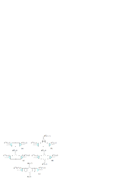
Figure 1: (Color online) Diagrammatic representation of the effective action, Eq. (43). (a) Conventional Ginzbirg-Landau functional $S_{GL}$. (b) Anomalous GE coupling between the scalar potential and the order parameter. (c) Gradient part of supercurrent action $S_{SC}$. (d) Diamagnetic component of the supercurrent. (e) Nonlocal MT term (here $\tau=(t+t^{\prime})/2$ and there are two possibilities: one vector potential classical and another quantum, which is part of the current, or two quantum, which is FDT counterpart).

The TDGL part of the action $S_{GL}[\vec{\Delta}_{\mathcal{K}},\mathbf{A}_{\mathcal{K}}^{cl}]$ has a local form standard for the Keldysh formalism. It comes from $\mathrm{Tr}[\vec{V}^{\dagger}\mathcal{C}\vec{V}]$ and $\mathrm{Tr}[\vec{V}^{\dagger}\bar{\mathcal{C}}\vec{V}]$ terms, Fig. 1(a)

$$S_{GL}=\frac{\pi\nu}{8T}\,\,\mathrm{Tr}\left[\vec{\Delta}^{{\dagger}}_{\mathcal{K}}(\mathbf{r},t)\hat{L}^{-1}\,\vec{\Delta}_{\mathcal{K}}(\mathbf{r},t)\right]\ ,$$ (44)

where the fluctuations propagator $\hat{L}$ has a typical bosonic form in the Keldysh space

$$\hat{L}^{-1}=\left(\begin{array}[]{cc}0&L^{-1}_{A}\\ L^{-1}_{R}&4iT\end{array}\right).$$ (45)

Here, retarded and/or advanced components of the fluctuation propagator are given by

$$L^{-1}_{R(A)}=\mp\partial_{t}-\tau^{-1}_{GL}+D\left[\nabla-2ie\mathbf{A}^{cl}_{\mathcal{K}}(\mathbf{r},t)\right]^{2}\,,$$ (46)

while Keldysh component of the propagator satisfy the FDT in equilibrium $L_{K}^{-1}=B_{\omega}\left(L^{-1}_{R}-L^{-1}_{A}\right)\to 4iT$ if $\omega\ll T$. Note that the scalar potential ${\Phi}_{\mathcal{K}}^{cl}$, although present in the action (38) through the operators (41a) and (41b), does not show up in the Ginzburg-Landau action (44). This happens because upon substitution of the Cooperon generators by their saddle point values (42) the terms $\Phi_{\mathcal{K}}^{cl}(\mathbf{r},t)$ and $\Phi_{\mathcal{K}}^{cl}(\mathbf{r},t^{\prime})$ in Eqs. (41a) and (41b) cancel each other. [To be precise there is a small residual term $\sim\partial_{t}\Phi_{\mathcal{K}}^{cl}/T$, which we do not keep, since it exceeds the accuracy of our calculations. For the same reason, terms with $\Phi_{\mathcal{K}}^{q}$ are not kept in the $\mathcal{N}$ operator Eq. (41c)]. As a result, the effective TDGL action depends only on the vector potential, but not on the scalar potential, if written in the $\mathcal{K}$-gauge. In any other gauge, there is a linear coupling between the scalar potential and the $z$-diffuson mode $\sim F\Phi^{cl}\bar{w}^{z}+\Phi^{q}w^{z}$, cf. Eq. (28). Taken together with the terms $\Delta\bar{w}w^{z}$ and $\Delta w\bar{w}^{z}$ (see next subsection) and being averaged over the diffuson fluctuations, these terms lead to a nonlocal coupling between the scalar potential $\Phi$ and the order parameter $|\Delta|^{2}$, see Fig. 1(b). This is the anomalous GE term. Thanks to the condition (28) the anomalous term is absent in the $\mathcal{K}$-gauge, making this gauge especially convenient to work in.

The supercurrent action $S_{SC}[\vec{\Delta}_{\mathcal{K}},\vec{\mathbf{A}}_{\mathcal{K}}]$ comes from the diagonal terms in Eq. (38) $\mathrm{Tr}[w\mathcal{N}w]$ and $\mathrm{Tr}[\bar{w}\mathcal{N}\bar{w}]$, where Cooperon generators $w$ and $\bar{w}$ are given by Eq. (42). It is also local and given by

$$S_{SC}=\frac{\pi e\nu D}{2T}\,\,\mathrm{Tr}\left\{\mathbf{A}^{q}_{\mathcal{K}}\mathrm{Im}\left[\Delta^{*cl}_{\mathcal{K}}(\nabla-2ie\mathbf{A}^{cl}_{\mathcal{K}})\Delta^{cl}_{\mathcal{K}}\right]\right\}\,.$$ (47)

The gradient part of the supercurrent originates from $\frac{1}{2}\,\mbox{div}\,\mathbf{A}^{q}_{\mathcal{K}}+\mathbf{A}^{q}_{\mathcal{K}}\nabla$ terms in the rhs of Eq. (41c), while the diamagnetic current originates from $2ie\mathbf{A}^{q}_{\mathcal{K}}\mathbf{A}^{cl}_{\mathcal{K}}$ term, see Figa. 1(c) and 1(d).

Time locality of the Ginzburg-Landau and the supercurrent actions stems from their diagonal nature. Indeed, they both involve products such as $w_{t,t^{\prime}}w_{t^{\prime},t}$. According to Eqs. (39) and (42), $w_{t,t^{\prime}}\sim\tilde{\theta}(t-t^{\prime})$, where $\tilde{\theta}(t)$ is the step function smeared at the scale $1/T$. Therefore, the time variables in $w_{t,t^{\prime}}w_{t^{\prime},t}$ are compatible only in the narrow vicinity of $t=t^{\prime}$, i.e., $|t-t^{\prime}|\lesssim 1/T$, hence the time locality. This argument does not apply to the off-diagonal MT term. Indeed, the latter involves product of retarded and advanced generators $w_{t,t^{\prime}}\bar{w}_{t^{\prime},t}$ whose time variables are compatible for any $t>t^{\prime}$.

The Maki-Thompson action $S_{MT}[\Delta_{\mathcal{K}}^{cl},\vec{\mathbf{A}}_{\mathcal{K}}]$, coming from the off-diagonal blocks of $\hat{\mathfrak{C}}^{-1}$ operator, has essentially time nonlocal form as explained above, Fig. 1(e),

$$S_{MT}=e^{2}\nu\,\mathrm{Tr}\left[\vec{\mathbf{A}}^{{\dagger}}_{\mathcal{K}}(\mathbf{r},t)\hat{\mathcal{T}}_{\delta D}(t,t^{\prime})\vec{\mathbf{A}}_{\mathcal{K}}(\mathbf{r},t^{\prime})]\right]\,,$$ (48)

where the operator $\hat{\mathcal{T}}_{\delta D}(t,t^{\prime})$ is given by [cf. Eq. (32)]

$$\hat{\mathcal{T}}_{\delta D}=\left(\begin{array}[]{cc}0&-\overleftarrow{\partial_{t}}\,\delta D^{MT}_{\mathbf{r},t^{\prime},t}\\ -\delta D^{MT}_{\mathbf{r},t,t^{\prime}}\,\overrightarrow{\partial_{t^{\prime}}}&2iT\left(\delta D^{MT}_{\mathbf{r},t,t^{\prime}}+\delta D^{MT}_{\mathbf{r},t^{\prime},t}\right)\end{array}\right),$$ (49)

where the $\delta D^{MT}[\Delta_{\mathcal{K}}^{cl}]$ functional is given by Eq. (14). Note that the MT action has exactly the same structure as the second term in the normal action (31). It therefore amounts to the time nonlocal renormalization of the normal diffuson constant $D\delta_{t-t^{\prime}}\to D\delta_{t-t^{\prime}}+\delta D^{MT}_{\mathbf{r},t,t^{\prime}}$.

Finally, we comment on the so called density of states (DOS) contributions. Larkin-Varlamov They originate from the subleading terms (in characteristic frequency over temperature) in the diagonal operator $\mathcal{N}$ [not written explicitly in Eq. (41c)], see Appendix B.3 for details. Accounting for them leads to a local renormalization of the density of states prefactor in the normal action, Eq. (31), or Eq. (33),

$$\nu\rightarrow\nu_{\mathbf{r},t}=\nu\left[1-\frac{7\zeta(3)}{4\pi^{2}T^{2}}\,|\Delta^{cl}_{\mathcal{K}}(\mathbf{r},t)|^{2}\right],$$ (50)

where $\zeta(x)$ is the Riemann zeta function. This is a small effect in the regime we are working in.

III.4 Nonlinear terms in the Ginzburg-Landau functional

The nonlinear in $\Delta$ terms of the TDGL equation are not very significant at $T>T_{c}$. Nevertheless, we shall discuss them here for completeness. There are several ways “$|\Delta|^{4}$” terms appear in the effective TDGL action. We shall keep track of $\Delta^{*q}\Delta^{cl}|\Delta^{cl}|^{2}$ terms which directly contribute to TDGL equation for $\Delta^{cl}$, discussing other combinations only briefly. The most important way such terms appear is through the third order expansion of the $\mathrm{Tr}[\check{\Delta}_{\mathcal{K}}\check{Q}_{\mathcal{K}}]$ term of the $\sigma$-model action (20c) in powers of $\check{W}$. Keeping only the Cooperon generators and employing $\mathrm{Tr}[\tau_{\pm}\tau_{z}\tau_{\mp}\tau_{\pm}\tau_{\mp}]=\mp 1$, one obtains

$$S_{NL}=\frac{\pi\nu}{12}\,\mathrm{Tr}\left[\Delta^{cl}_{\mathcal{K}}\left(w^{*}ww^{*}-\bar{w}^{*}\bar{w}\bar{w}^{*}\right)+c.c.\right].$$ (51)

Similar terms coming with $\Delta^{q}_{\mathcal{K}}$ component of the order parameter eventually cancel out between $w$ and $\bar{w}$ contributions and thus are omitted in Eq. (51). Next, one substitutes the saddle point value of the Cooperon generators Eq. (42) into the action (51), and perform traces over the time indices. In doing so, one should keep only the first power of the quantum component of the order parameter [coming from Eq. (39)]. The diagrammatic representation of the corresponding terms is shown in Fig. 2(a). After straightforward algebra (see Appendix C for details), one finds

$$S_{NL}=-\frac{7\zeta(3)\nu}{8\pi^{2}T^{2}}\,\mathrm{Tr}\left[\Delta^{*q}_{\mathcal{K}}(\mathbf{r},t)\Delta^{cl}_{\mathcal{K}}(\mathbf{r},t)|\Delta^{cl}_{\mathcal{K}}(\mathbf{r},t)|^{2}+c.c.\right].$$ (52)

This term is to be added to the retarded and advanced (but not Keldysh) parts of the Ginzburg-Landau action (44). It leads to the standard nonlinear term of the Ginzburg-Landau equation, Abrikosov ; Larkin-Varlamov which is (a) local, (b) disorder independent, in agreement with Anderson theorem.

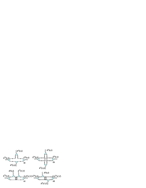
Figure 2: (Color online) Nonlinear contributions to Ginzburg-Landau functional. (a) Diagram for the local nonlinear term of the action Eq.(52). (b) Renormalization of the diffusion constant in the TDGL equation – shaded square is the Hikami box. [(c) and (d)] terms involving diffuson channel, leading to a nonlocal renormalization of the dynamic part in TDGL equation.

Interestingly, this is not the only way the nonlinear terms appear in the effective action. Let us mention two other venues. (i) One may expand the $D\ \mathrm{Tr}[\nabla\check{Q}_{\mathcal{K}}]^{2}$ term of the nonlinear $\sigma$ model action (20c) to the fourth order in the Cooperon fields, generating the so-called Hikami box, see Fig. 2(b). One then substitutes the saddle point value of the Cooperon generators (42) in such a term to obtain a contribution quartic in the order parameter. This term leads to a local renormalization of the diffusion constant in TDGL equation $\delta D_{\mathbf{r},t}\sim D|\Delta^{cl}(\mathbf{r},t)|^{2}/T^{2}$. There is no MT nonlocal renormalization of the diffusion constant in the superconductive part of the action (as opposed to the normal one where both MT and DOS renormalizations take place). (ii) There is yet another source of nonlinear terms (we are not aware if it had been discussed previously in the literature). It originates as a result of mixing between Cooperon and diffuson channels. To see it, one expands $\mathrm{Tr}[\check{\Delta}_{\mathcal{K}}\check{Q}_{\mathcal{K}}]$ term of the $\sigma$-model action (20c) to the second order in $\check{W}$. This way one generates interaction vertices of the following structure $\mathrm{Tr}[\check{\Delta}_{\mathcal{K}}w^{*}({w}^{\alpha}\pm\bar{w}^{\alpha})]+c.c.$ with $\alpha=0,z$ and corresponding terms with $\bar{w}$. We then perform Gaussian integration over the diffuson fields $w^{\alpha},\bar{w}^{\alpha}$ to obtain a nonlocal vertex $\mathrm{Tr}[w^{*}_{tt^{\prime}}\check{\Delta}_{\mathcal{K}}(\mathbf{r},t^{\prime})\langle w^{\alpha}_{t^{\prime}t}\bar{w}^{\alpha}_{\tilde{t}\tilde{t}^{\prime}}\rangle\check{\Delta}_{\mathcal{K}}^{*}(\mathbf{r}^{\prime},\tilde{t}^{\prime})w_{\tilde{t}^{\prime}\tilde{t}}]$, where $\langle w^{\alpha}\bar{w}^{\alpha}\rangle$ is the diffuson propagator, Eq. (11). There is a similar vertex with $\bar{w}^{*},\bar{w}$ generators. Such a nonlocal vertex is effectively a renormalization of the diagonal part of the $\hat{\mathfrak{C}}^{-1}_{tt^{\prime}}$ operator in Eq. (38). It is important to stress that the diffuson admixture does not generate the off-diagonal terms in $\hat{\mathfrak{C}}^{-1}_{tt^{\prime}}$ operator, thus not affecting directly the MT channel. We then substitute the saddle point values of the Cooperon generators, Eq. (42), in this nonlocal vertex and find

$$\widetilde{S}_{NL}=\frac{7\zeta(3)\nu}{8\pi^{2}T^{2}}\mathrm{Tr}\ [\Delta^{*q}_{\mathcal{K}}(\mathbf{r},t)\Delta^{cl}_{\mathcal{K}}(\mathbf{r},t)\mathcal{D}^{\mathbf{r},\mathbf{r}^{\prime}}_{t,t^{\prime}}\Delta^{*cl}_{\mathcal{K}}(\mathbf{r}^{\prime},t^{\prime})\,\partial_{t^{\prime}}\Delta^{cl}_{\mathcal{K}}(\mathbf{r}^{\prime},t^{\prime})+c.c.]\,.$$ (53)

This term is formally of the same order of magnitude as the conventional one, Eq. (52). Indeed, the diffuson propagator $\mathcal{D}^{\mathbf{r},\mathbf{r}^{\prime}}_{t,t^{\prime}}$ is not cut by the temperature [unlike the Cooperon propagators in Fig. 2b].

III.5 Equations of motion and Coulomb interactions

To derive the stochastic equations of motion presented in Sec. II, one needs to get rid of terms quadratic in quantum components of the fields: $\Delta_{\mathcal{K}}^{q}$ in $S_{GL}$ and $\mathbf{A}_{\mathcal{K}}^{q}$ in $S_{N}+S_{MT}$. This is achieved with the Hubbard-Stratonovich transformation similar to Eq. (34) for $\mathbf{A}_{\mathcal{K}}^{q}$ and

$$e^{-{\pi\nu\over 2}\mathrm{Tr}|\Delta^{q}_{\mathcal{K}}|^{2}}=\int\mathrm{D}[\xi_{\Delta}]e^{-\frac{\pi\nu}{8T}\mathrm{Tr}\left[\frac{|\xi_{\Delta}|^{2}}{4T}-i\xi^{*}_{\Delta}\Delta^{q}_{\mathcal{K}}-i\xi_{\Delta}\Delta^{*q}_{\mathcal{K}}\right]}$$ (54)

for $\Delta_{\mathcal{K}}^{q}$. As a result, the effective action (43) acquires the form linear in quantum components of the fields. Integration over the latter leads to the functional delta functions imposing the stochastic equations of motion. This way the TDGL equation (8), which we present here including the nonlinear terms

$$\left[\partial_{t}+\tau^{-1}_{GL}-D(\nabla-2ie\mathbf{A}_{\mathcal{K}}(\mathbf{r},t))^{2}+{b\over T}|\Delta_{\mathcal{K}}(\mathbf{r},t)|^{2}-{b\over T}\!\int\!\mathrm{d}t^{\prime}\mathrm{d}\mathbf{r}^{\prime}\Delta^{*}_{\mathcal{K}}(\mathbf{r}^{\prime},t^{\prime})\partial_{t^{\prime}}\Delta_{\mathcal{K}}(\mathbf{r}^{\prime},t^{\prime})\,\mathcal{D}^{\mathbf{r},\mathbf{r}^{\prime}}_{t,t^{\prime}}\right]\Delta_{\mathcal{K}}(\mathbf{r},t)=\xi_{\Delta}(\mathbf{r},t)$$ (55)

with $b=7\zeta(3)/\pi^{3}$, the continuity equation (12), and expression for the current (13) are obtained for the classical components of the fields (we have omitted the subscript $cl$ for brevity). The correlators of the Gaussian noise sources may be directly read out from the Hubbard-Stratonovich procedure and are given by Eqs. (5) and (16).

We discuss briefly the role of the last nonlinear term in the lhs of TDGL equation (55). On the mean-field level, i.e., being averaged over the fluctuations of the order parameter $\langle\Delta^{cl}_{\mathcal{K}}(\mathbf{r},t)\Delta^{*cl}_{\mathcal{K}}(\mathbf{r}^{\prime},t^{\prime})\rangle\propto L_{K}(\mathbf{r}-\mathbf{r}^{\prime},t-t^{\prime})$, this term leads to a renormalization of the coefficient in front of the time derivative (8),

$$\partial_{t}\Delta_{\mathcal{K}}\rightarrow\left(1-c_{d}\,\frac{[\xi(T)]^{4-d}}{\nu D\xi_{0}^{2}}\right)\partial_{t}\Delta_{\mathcal{K}}\,,$$ (56)

where $\xi_{0}=\sqrt{D/T_{c}}$ and $\xi(T)=\sqrt{D/(T-T_{c})}$. The dimensionality dependent coefficient $c_{d}$ appears as the result of the convolution between the diffuson and the Keldysh components of the fluctuations propagator and reads as

$$c_{d}=\frac{7\zeta(3)}{8\pi^{3}}\int\frac{\mathrm{d}^{d}k}{(2\pi)^{d}}\frac{1}{(k^{2}+1)(k^{2}+1/2)},$$ (57)

here is $c_{1}=0.044$, $c_{2}=0.012$, and $c_{3}=0.005$. Note that disorder-dependent renormalization of the $\partial_{t}\Delta_{\mathcal{K}}$ term does not violate Anderson theorem. The down renormalization of the coefficient in front of the first time derivative is a precursor of the oscillatory Carlson-Goldman CG modes, appearing below $T_{c}$.

Finally, the TDGL equation (8), written in the $\mathcal{K}$-gauge may be transformed to an arbitrary gauge by the substitution $\Delta_{\mathcal{K}}=\Delta e^{-2ie\mathcal{K}}$. Such a substitution brings the vector potential $\mathbf{A}$ to the covariant spatial derivative, while the the time derivative acquires the anomalous GE term $\partial_{t}\to\partial_{t}-2ie\partial_{t}\mathcal{K}$. This way TDGL equation (2) is obtained.

The set of equations is simplified in the limit of the strong Coulomb interactions. Gorkov-Eliashberg The latter impose the condition of local instantaneous charge neutrality $\rho(\mathbf{r},t)=0$ and therefore $\,\mbox{div}\ \mathbf{j}=0$. Applying this condition to the expression for the current (13) and neglecting for simplicity the MT and supercurrent contributions, one finds $e^{2}\nu D\,\mbox{div}\ \mathbf{E}=\,\mbox{div}\ \xi_{\mathbf{j}}$. As a result, the longitudinal component of the electric filed $\mathbf{E}_{\parallel}$ is a fluctuating Gaussian field. Employing Eqs. (10) and (16), one may translate it to the Gaussian correlator for the longitudinal component of the vector $\mathbf{A}_{\parallel\mathcal{K}}(\mathbf{r},t)=\mathbf{A}_{\parallel\mathcal{K}}^{ext}(t)+\mathbf{A}_{\parallel\mathcal{K}}^{fluct}(\mathbf{r},t)$, where $\mathbf{A}_{\parallel\mathcal{K}}^{ext}(t)$ is an externally applied divergenceless field and the fluctuation component has the correlator

$$\left\langle\mathbf{A}_{\parallel\mathcal{K}}^{fluct}(\mathbf{-q},-\omega)\mathbf{A}_{\parallel\mathcal{K}}^{fluct}(\mathbf{q},\omega)\right\rangle=\frac{2T}{e^{2}\nu D}\,\frac{1}{(D\mathbf{q}^{2})^{2}+\omega^{2}}\,.$$ (58)

Exactly the same expression may be, of course, directly read out from the normal action (33) (the Maxwell part of the action is absent in the the strong Coulomb limit). To this end, one needs to perform the Gaussian integration over the $\mathbf{A}_{\mathcal{K}}^{q}$ component leading to the quadratic action for the $\mathbf{A}_{\mathcal{K}}^{cl}$ with the correlator given by Eq. (58). It is this fluctuating vector potential which is responsible for dephasing of the Cooperon propagators. AAK

III.6 Effective action versus diagrammatic technique

Given that there is an existing microscopic formalism for the Aslamazov-Larkin, Maki-Thompson, and density of states diagrams, it is important that the results from the Keldysh effective action, formulated in the previous sections, be compared with well established results for the corrections to the conductivity. This comparison is the necessary check for the validity of our approach.

We start from the density of states contribution to the conductivity. For that purpose, one uses Eq.(50) and writes conductivity correction in the form

$$\delta\sigma_{DOS}=e^{2}D\left\langle\delta\nu^{DOS}_{\mathbf{r},t}\right\rangle_{\Delta}=-\frac{7\zeta(3)e^{2}\nu D}{4\pi^{2}T^{2}_{c}}\left\langle|\Delta^{cl}_{\mathcal{K}}(\mathbf{r},t)|\right\rangle_{\Delta}.$$ (59)

The averaging over the order parameter fluctuations is done easily in the momentum space $\left\langle|\Delta^{cl}_{\mathcal{K}}(\mathbf{r},t)|\right\rangle_{\Delta}=\frac{8T_{c}}{\pi\nu}\sum_{\mathbf{q}\omega}L_{K}(\mathbf{q},\omega)$. Using then explicit form of the Keldysh component for the fluctuations propagator (45), one finds

$$\delta\sigma_{DOS}=-\frac{28\zeta(3)}{\pi^{4}}\ e^{2}D\sum_{\mathbf{q}}\int\limits^{+\infty}_{-\infty}\mathrm{d}\omega\frac{1}{(D\mathbf{q}^{2}+\tau^{-1}_{GL})+\omega^{2}}.$$ (60)

Further analysis of the formula (60) depends essentially on the system effective dimensionality. As an example, let us concentrate on the quasi-two-dimensional geometry – metal film with the thickness $d$, which is much smaller than the superconductive coherence length $d\ll\xi(T)$. In this case, momentum sum can be written as the integral according to the substitution $\sum_{\mathbf{q}}\rightarrow\frac{1}{d}\int\frac{\mathrm{d}\mathbf{q}^{2}}{4\pi}$. Performing remaining integrations, with the logarithmic accuracy one finds

$$\delta\sigma_{DOS}=-\frac{7\zeta(3)e^{2}}{\pi^{4}d}\ln\left(\frac{T_{c}}{T-T_{c}}\right).$$ (61)

Deriving Eq.(61), the momentum integration was cut at the upper limit $D\mathbf{q}^{2}_{\mathrm{max}}\sim T_{c}$. Recall that effective action was derived under the constraint $D\mathbf{q}^{2}\sim\omega\ll T_{c}$, thus such a regularization is self-consistent.

We proceed with the Maki-Thompson correction to the conductivity. In this case, one starts from the formula $\delta\sigma_{MT}=e^{2}\nu\left\langle\delta D^{MT}_{\mathbf{r},t}\right\rangle_{\Delta}$, uses explicit form of the $\delta D^{MT}_{\mathbf{r},t}$ given by Eq. (14), and rewrites average over $\Delta$ in the momentum space. This way one obtains

$$\delta\sigma_{MT}=\frac{4}{\pi}\ e^{2}D\sum_{\mathbf{q}}\int\mathrm{d}\omega\frac{T_{c}}{D\mathbf{q}^{2}[(D\mathbf{q}^{2}+\tau^{-1}_{GL})^{2}+\omega^{2}]}.$$ (62)

Again in the case of the two dimensional geometry, after momentum and frequency integrations, Eq, (62) reduces to

$$\delta\sigma_{MT}=\frac{e^{2}}{8d}\left(\frac{T_{c}}{T-T_{c}}\right)\ln\left(\frac{\tau_{\phi}}{\tau_{GL}}\right),$$ (63)

where infrared divergency in the momentum integration was cut here by hand introducing dephasing time $D\mathbf{q}^{2}_{\mathrm{min}}\sim\tau^{-1}_{\phi}$. This spurious divergency is very well known feature of the Maki-Thompson diagram. It was regularized by Thompson introducing magnetic impurities, and in that case dephasing time $\tau_{\phi}$ is nothing else but the spin flip time $\tau_{s}$.

Finally, we summarize with few additional remarks. Equations (60) and (62) can be recovered from the traditional Matsubara diagrammatic techniques after one expands all fluctuation propagators at small frequencies and momenta, integrates fast fermionic energies, and keeps only contribution from zero Matsubara frequency [in our language, latter condition strictly speaking corresponds to the long time approximation for the distribution function Eq.(26)]. To this extent, effective action approach contains the most divergent temperature part of the conductivity corrections, thus allows to reproduce known results.

IV Discussion

We have presented a systematic way to integrate out the fermionic degrees of freedom in a fluctuating superconductor. The underlying assumptions for this procedure are: (i) spatial and temporal scales of all bosonic fields are slow in comparison with $\xi_{0}$ and $1/T_{c}$ correspondingly (but not necessarily slow in comparison with $\xi(T)=\xi_{0}\sqrt{T_{c}/(T-T_{c})}$ and $\tau_{GL}$). (ii) The external electromagnetic fields are sufficiently small (see Sec. I for the details), such that the fermionic degrees of freedom are in local equilibrium. The result is the dynamic Keldysh action written in terms of the fluctuating order parameter and electromagnetic potentials. This action naturally incorporates (time nonlocal) MT terms as well as anomalous GE terms, effectively closing the discussion whether or not TDGL theory includes the MT effect. We have also uncovered certain nonlocal nonlinear terms of TDGL equation (passed previously unnoticed, to the best of our knowledge). The nonlinear coupling of the electromagnetic fields, leading to the Altshuler-Aronov effect, may be also directly incorporated into the scheme.

Although we did not evaluate any physical observable here, the derived action opens the way to describe a number of phenomena. To name a few, we mention, e.g., nonequilibrium current noise in proximity to the critical temperature, especially the MT contribution to noise, which would be very difficult to calculate by any other mean. Another possible application is evaluation of the MT dephasing time. Extension of the theory for $T<T_{c}$ to describe, e.g., the collective modes CG and analysis of the dynamical regimes far from the equilibrium, are yet another fascinating directions.

We are grateful to L. Glazman, B. Ivlev, M. Khodas, I. Lerner and A. Varlamov for useful discussions. This work is supported by the NSF Grant Nos. DMR 02-37296, DMR 04-39026, and DMR 0405212. A.K. is also supported by the A. P. Sloan foundation.

Appendix A Diffuson expansion and normal action

We first focus on the part of the action (20) which is linear in the electromagnetic potentials. There are two such terms: $S_{\Phi}$ originating from the trace $\mathrm{Tr}[\check{\Phi}_{\mathcal{K}}\check{Q}_{\mathcal{K}}]$ and $S_{\mathbf{A}}$ coming from the covariant derivative (21). We then expand $\check{Q}_{\mathcal{K}}$ matrix to the linear order in deviations from the saddle point $\check{Q}_{\mathcal{K}}=\check{\Lambda}+\frac{1}{2}[\check{\Lambda},\check{W}]+\ldots$, and use the cyclic property of the trace operation to obtain $S_{\Phi}=-\frac{\pi e\nu}{4}\mathrm{Tr}\left([\check{\Phi}_{\mathcal{K}},\check{\Lambda}]\check{W}\right)$ and $S_{\mathbf{A}}=\frac{\pi e\nu D}{4}\mathrm{Tr}\left(\check{\Lambda}\nabla\check{W}[\check{\Xi}\check{\mathbf{A}}_{\mathcal{K}},\check{\Lambda}]\right)$ which after the integration by parts translates into $S_{\mathbf{A}}=-\frac{\pi e\nu D}{4}\mathrm{Tr}\left(\check{\Xi}\nabla\check{\mathbf{A}}_{\mathcal{K}}-\check{\Lambda}\check{\Xi}\nabla\check{\mathbf{A}}_{\mathcal{K}}\check{\Lambda}\right)\check{W}$. Requiring that terms linear in variation $\check{W}$ (and linear in potentials) vanish, one arrives at Eq (28).

Expanding action (20) to the second order in $\check{W}$ and keeping track of the diffusons only, one finds quadratic action of the diffuson degrees of freedom

$$iS_{D}[w^{0},w^{z}]=\frac{\pi\nu}{2}\mathrm{Tr}\left\{\bar{w}^{\alpha}_{tt^{\prime}}[-D\nabla^{2}+\partial_{t}+\partial_{t^{\prime}}]w^{\alpha}_{t^{\prime}t}\right\}\,,$$ (64)

where $\alpha=0,z$. This action leads to the following propagator:

$$\langle w^{\alpha}_{\varepsilon_{1},\varepsilon_{2}}(\mathbf{q})\bar{w}^{\alpha}_{\varepsilon_{3},\varepsilon_{4}}(-\mathbf{q})\rangle=-\frac{2}{\pi\nu}\frac{(2\pi)^{2}\delta_{\varepsilon_{1}-\varepsilon_{4}}\delta_{\varepsilon_{2}-\varepsilon_{3}}}{D\mathbf{q}^{2}-i(\varepsilon_{1}-\varepsilon_{2})}\,.$$ (65)

Substituting the saddle point $\check{\Lambda}$ in the $\sigma$-model action (20), one finds

$$S_{N} = \frac{e^{2}\nu}{2}\,\mathrm{Tr}\left\{\check{\Phi}_{\mathcal{K}}\check{\Upsilon}\check{\Phi}_{\mathcal{K}}\right\}$$

$$- \frac{i\pi e^{2}\nu D}{4}\mathrm{Tr}\,\left\{\check{\Xi}\check{\mathbf{A}}_{\mathcal{K}}\check{\Lambda}\check{\Xi}\check{\mathbf{A}}_{\mathcal{K}}\check{\Lambda}-\check{\Xi}\check{\mathbf{A}}_{\mathcal{K}}\check{\Xi}\check{\mathbf{A}}_{\mathcal{K}}\right\}\,.$$

The traces are evaluated using the following matrix identity:

$$\int\limits^{+\infty}_{-\infty}\mathrm{d}\epsilon\ \mathrm{Tr}\left[\check{\Upsilon}_{\alpha}\check{\Upsilon}_{\beta}-\check{\Upsilon}_{\alpha}\check{\Lambda}_{\epsilon_{+}}\check{\Upsilon}_{\beta}\check{\Lambda}_{\epsilon_{-}}\right]=8\omega(\hat{\Pi}^{-1}_{\omega})_{\alpha\beta}\,,$$ (67)

where

$$\hat{\Pi}^{-1}_{\omega}=\!\left(\begin{array}[]{cc}0&-1\\ 1&2B_{\omega}\end{array}\right)$$ (68)

and $\check{\Upsilon}_{1}=\sigma_{0}\otimes\tau_{z}$, $\check{\Upsilon}_{2}=\sigma_{x}\otimes\tau_{z}$, $\epsilon_{\pm}=\epsilon\pm\omega/2$. The identity is based on the relation between the bosonic and fermionic distribution functions:

$$\int\limits^{+\infty}_{-\infty}\mathrm{d}\epsilon(F_{\epsilon_{+}}-F_{\epsilon_{-}})=2\omega,$$ (69a)

$$\int\limits^{+\infty}_{-\infty}\mathrm{d}\epsilon(1-F_{\epsilon_{+}}F_{\epsilon_{-}})=2\omega B_{\omega}.$$ (69b)

Combining Eqs. (A)-(69), we arrive at normal metal action (31). Finally, to find the macroscopic equations (12) and (36), one needs to express gauged electromagnetic potentials $\Phi_{\mathcal{K}},\mathbf{A}_{\mathcal{K}}$ in terms of bare ones $\Phi,\mathbf{A}$. Using Eq. (29), one may find the relation between those

$$\vec{\mathbf{A}}_{\mathcal{K}}(\mathbf{q},\omega)=\vec{\mathbf{A}}_{\perp}(\mathbf{q},\omega)-i\mathbf{q}\hat{\mathcal{D}}^{\,\mathbf{q}}_{\omega}\hat{\Pi}^{-1}_{\omega}[\vec{\Phi}+\omega(\mathbf{q}\vec{\mathbf{A}}_{\parallel})/\mathbf{q}^{2}],$$ (70a)

$$\vec{\Phi}_{\mathcal{K}}(\,\mathbf{q},\omega)=D\mathbf{q}^{2}\hat{\mathcal{D}}^{\mathbf{q}}_{\omega}\sigma_{x}[\vec{\Phi}+\omega(\mathbf{q}\vec{\mathbf{A}}_{\parallel})/\mathbf{q}^{2}],$$ (70b)

where

$$\hat{\mathcal{D}}^{\,\mathbf{q}}_{\omega}=\frac{1}{(D\mathbf{q}^{2})^{2}+\omega^{2}}\!\left(\!\begin{array}[]{cc}2i\omega B_{\omega}&\!\!i\omega+D\mathbf{q}^{2}\\ -i\omega+D\mathbf{q}^{2}&0\end{array}\right).$$ (71)

Appendix B Cooperon expansion and effective action

Carrying out the Cooperon expansion, it is convenient to distinguish several contributions into the $\sigma$-model action (20):

$$S_{\sigma}[W,\vec{\Delta}_{\mathcal{K}},\vec{\Phi}_{\mathcal{K}},\vec{\mathbf{A}}_{\mathcal{K}}] = S^{a}_{\sigma}[W]+S^{b}_{\sigma}[W,\vec{\Delta}_{\mathcal{K}}]$$

$$+ S^{c}_{\sigma}[W,\vec{\mathbf{A}}_{\mathcal{K}}]+S^{d}_{\sigma}[W,\vec{\mathbf{A}}_{\mathcal{K}}].$$

The $S^{a}_{\sigma}[W]$ part corresponds to the free Cooperons which are uncoupled from both $\Delta_{\mathcal{K}}(\mathbf{r},t)$ and $\mathbf{A}_{\mathcal{K}}(\mathbf{r},t)$. This contribution arises after one expands trace of the gradient term $\mathrm{Tr}(\nabla\check{Q})^{2}=\mathrm{Tr}(\check{\Lambda}\nabla\check{W}\check{\Lambda}\nabla\check{W})=\mathrm{Tr}(\check{\mathcal{W}}\nabla^{2}\check{\mathcal{W}})$ and trace of the time derivative term $\mathrm{Tr}[\check{\Xi}\partial_{t}\check{Q}]=\frac{1}{2}\mathrm{Tr}[\check{\Xi}\partial_{t}\check{\Lambda}\check{W}^{2}]=\frac{1}{2}\mathrm{Tr}[\check{\Xi}\partial_{t}\check{\mathcal{U}}\check{\Lambda}_{0}\check{\mathcal{W}}\check{\mathcal{W}}\check{\mathcal{U}}]$. Multiplying matrices, tracing them over Keldysh-Nambu space, one finds

$$S^{a}_{\sigma}[W]=\frac{i\pi\nu}{4}\mathrm{Tr}\{w^{*}_{tt^{\prime}}[-D\nabla^{2}-\partial_{t}+\partial_{t^{\prime}}]w_{t^{\prime}t}+(w\rightarrow\bar{w})\}.$$ (73)

The $S^{b}_{\sigma}[W,\Delta_{\mathcal{K}}]$ part corresponds to the coupling term between Cooperons and the order parameter. This contribution arises from the trace $\mathrm{Tr}[\check{\Delta}_{\mathcal{K}}\check{Q}_{\mathcal{K}}]$ after one expands $\check{Q}_{\mathcal{K}}$ to the first order in $\check{W}$: $\mathrm{Tr}[\check{\Delta}_{\mathcal{K}}\check{Q}_{\mathcal{K}}]=\mathrm{Tr}[\check{\Delta}_{\mathcal{K}}\check{\Lambda}\check{W}]=\mathrm{Tr}[\check{\mathcal{U}}\check{\Delta}_{\mathcal{K}}\check{\mathcal{U}}\check{\Lambda}_{0}\check{\mathcal{W}}]$. After evaluation of traces, which is done with the help of the identity $\mathrm{Tr}_{N}[\tau_{\pm}\tau_{z}\tau_{\mp}]=\mp 1$, one finds

$$S^{b}_{\sigma}[W,\vec{\Delta}_{\mathcal{K}}]=\frac{\pi\nu}{2}\,\mathrm{Tr}\left[\vec{V}^{{\dagger}}_{tt^{\prime}}\vec{\mathfrak{W}}_{t^{\prime}t}-\vec{\mathfrak{W}}^{{\dagger}}_{tt^{\prime}}\vec{V}_{t^{\prime}t}\right],$$ (74)

where we have used vectors $\vec{\mathfrak{W}}$ and $\vec{V}$ in the notations of Eq. (38).

The c and d parts of the action are the terms which provide the interaction vertices between the cooperons $W$ and the vector potential $\mathbf{A}_{\mathcal{K}}$. The $S^{c}_{\sigma}[W,\mathbf{A}_{\mathcal{K}}]$ part is linear in the vector potential and arises from the square of the covariant derivative, keeping terms linear in $\mathbf{A}_{\mathcal{K}}$ contribution

$$S^{c}_{\sigma}=\frac{\pi e\nu D}{4}\mathrm{Tr}\{\nabla\check{Q}_{\mathcal{K}}[\check{\Xi}\check{\mathbf{A}}_{\mathcal{K}},\check{Q}_{\mathcal{K}}]\}=$$

$$\frac{\pi e\nu D}{4}\mathrm{Tr}\{\check{\Lambda}\nabla\check{W}[\check{\Xi}\check{\mathbf{A}}_{\mathcal{K}},\check{\Lambda}\check{W}]\}=\frac{\pi e\nu D}{4}\mathrm{Tr}\{\check{\mathcal{U}}\check{\Xi}\check{\mathbf{A}}_{\mathcal{K}}\check{\mathcal{U}}[\nabla\check{\mathcal{W}},\check{\mathcal{W}}]\}.$$

After a straightforward algebra, one finds

$$S^{c}_{\sigma}[W,\vec{\mathbf{A}}_{\mathcal{K}}]=-\frac{\pi e\nu D}{4}\mathrm{Tr}\{\mathcal{A}_{tt^{\prime\prime}}[w^{*}_{tt^{\prime}}\nabla w_{t^{\prime}t^{\prime\prime}}-\nabla w^{*}_{tt^{\prime}}w_{t^{\prime}t^{\prime\prime}}]$$ (75)

$$\qquad\qquad\qquad+\bar{\mathcal{A}}_{tt^{\prime\prime}}[\bar{w}^{*}_{tt^{\prime}}\nabla\bar{w}_{t^{\prime}t^{\prime\prime}}-\nabla\bar{w}^{*}_{tt^{\prime}}\bar{w}_{t^{\prime}t^{\prime\prime}}]-c.c.\}\,,$$

where we have introduced notations

$$\mathcal{A}_{tt^{\prime}}(\mathbf{r})=\delta_{t-t^{\prime}}\mathbf{A}^{cl}_{\mathcal{K}}(\mathbf{r},t)+\frac{i}{2T}\delta^{\prime}_{t^{\prime}-t}\mathbf{A}^{q}_{\mathcal{K}}(\mathbf{r},t)\ ,$$ (76a)

$$\bar{\mathcal{A}}_{tt^{\prime}}(\mathbf{r})=\delta_{t-t^{\prime}}\mathbf{A}^{cl}_{\mathcal{K}}(\mathbf{r},t)-\frac{i}{2T}\delta^{\prime}_{t^{\prime}-t}\mathbf{A}^{q}_{\mathcal{K}}(\mathbf{r},t^{\prime})\ .$$ (76b)

The quadratic in vector potential part of the action comes from the diamagnetic term, which has the form $S^{d}_{\sigma}[Q_{\mathcal{K}}]=-\frac{i\pi e^{2}\nu D}{4}\,\mathrm{Tr}\{\check{\Xi}\check{\mathbf{A}}_{\mathcal{K}}\check{Q}_{\mathcal{K}}\check{\Xi}\check{\mathbf{A}}_{\mathcal{K}}\check{Q}_{\mathcal{K}}\}$. One possibility is to expand one of the $\check{Q}_{\mathcal{K}}$ matrices up to the second order in $\check{W}$, while leaving the other to be $\check{\Lambda}$, the other is to expand both of them to the first order

$$S^{d}_{\sigma}[W,\vec{\mathbf{A}}_{\mathcal{K}}]=-\frac{i\pi e^{2}\nu D}{4}\mathrm{Tr}\,\left[\check{\Sigma}\check{\Sigma}\check{\mathcal{W}}\check{\mathcal{W}}+\check{\Sigma}\check{\mathcal{W}}\check{\Sigma}\check{\mathcal{W}}\right],$$ (77)

where

$$\check{\Sigma}_{\varepsilon\varepsilon^{\prime}}=\check{\mathcal{U}}_{\varepsilon}\check{\Xi}\check{\mathbf{A}}_{\varepsilon-\varepsilon^{\prime}}\check{\mathcal{U}}_{\varepsilon^{\prime}}\check{\Lambda}_{0}=$$ (78)

$$=\left[\begin{array}[]{cc}\mathbf{A}^{cl}_{\mathcal{K}}+F_{\varepsilon}\mathbf{A}^{q}_{\mathcal{K}}&\mathbf{A}^{q}_{\mathcal{K}}(1-F_{\varepsilon}F_{\varepsilon^{\prime}})+\mathbf{A}^{cl}_{\mathcal{K}}(F_{\varepsilon}-F_{\varepsilon^{\prime}})\\ -\mathbf{A}^{cl}_{\mathcal{K}}&-\mathbf{A}^{cl}_{\mathcal{K}}+F_{\varepsilon^{\prime}}\mathbf{A}^{q}_{\mathcal{K}}\end{array}\right],$$

and all vector potential have $\varepsilon-\varepsilon^{\prime}$ as an argument. Combining it with all the contributions, given by Eqs.(73)-(75), the full action may be conveniently presented using matrix notations as Eq. (38).

We turn now to the derivation of the effective action, Eq. (43). To this end, we transform Eq. (42) into the energy-momentum representation, then using explicit form of the $\vec{V}$ vector, given by the formula (39), we find for the Cooperon generators

$$w_{\varepsilon\varepsilon^{\prime}}(\mathbf{q})=-2i\frac{\Delta^{cl}_{\mathcal{K}}(\mathbf{q},\varepsilon-\varepsilon^{\prime})+F_{\varepsilon}\Delta^{q}_{\mathcal{K}}(\mathbf{q},\varepsilon-\varepsilon^{\prime})}{D\left(\mathbf{q}-2e\mathbf{A}^{cl}_{\mathcal{K}}\right)^{2}-i(\varepsilon+\varepsilon^{\prime})},$$ (79a)

$$\bar{w}_{\varepsilon\varepsilon^{\prime}}(\mathbf{q})=2i\frac{\Delta^{cl}_{\mathcal{K}}(\mathbf{q},\varepsilon-\varepsilon^{\prime})-F_{\varepsilon^{\prime}}\Delta^{q}_{\mathcal{K}}(\mathbf{q},\varepsilon-\varepsilon^{\prime})}{D\left(\mathbf{q}-2e\mathbf{A}^{cl}_{\mathcal{K}}\right)^{2}+i(\varepsilon+\varepsilon^{\prime})}.$$ (79b)

Note that the scale for the energy center of mass $\epsilon=(\varepsilon+\varepsilon^{\prime})/2$ is set by the temperature $\epsilon\sim T$. Then in most of the cases $D\mathbf{q}^{2}\sim\omega\sim T-T_{c}$ can be ignored as compared to $\epsilon$ (the exception is MT term), thus one may write instead of (79) the approximations

$$w_{\varepsilon\varepsilon^{\prime}}(\mathbf{q})\approx 2\frac{\Delta^{cl}_{\mathcal{K}}(\mathbf{q},\varepsilon-\varepsilon^{\prime})+F_{\varepsilon}\Delta^{q}_{\mathcal{K}}(\mathbf{q},\varepsilon-\varepsilon^{\prime})}{\varepsilon+\varepsilon^{\prime}+i0},$$ (80a)

$$\bar{w}_{\varepsilon\varepsilon^{\prime}}(\mathbf{q})\approx 2\frac{\Delta^{cl}_{\mathcal{K}}(\mathbf{q},\varepsilon-\varepsilon^{\prime})-F_{\varepsilon^{\prime}}\Delta^{q}_{\mathcal{K}}(\mathbf{q},\varepsilon-\varepsilon^{\prime})}{\varepsilon+\varepsilon^{\prime}-i0},$$ (80b)

and similar equations for the conjugated fields. After the inverse Fourier transform, one finds

$$w_{tt^{\prime}}(\mathbf{r})=-i\theta(t-t^{\prime})\Delta^{cl}_{\mathcal{K}}(\mathbf{r},\tau)+\Delta^{q}_{\mathcal{K}}(\mathbf{r},\tau)Y(t-t^{\prime}),$$ (81a)

$$\bar{w}_{tt^{\prime}}(\mathbf{r})=i\theta(t^{\prime}-t)\Delta^{cl}_{\mathcal{K}}(\mathbf{r},\tau)-\Delta^{q}_{\mathcal{K}}(\mathbf{r},\tau)Y(t-t^{\prime}),$$ (81b)

where $\tau=(t+t^{\prime})/2$ and

$$Y(t)=\int\limits^{+\infty}_{-\infty}\frac{\mathrm{d}\epsilon}{2\pi}\tanh\left[\frac{\epsilon}{2T}\right]\frac{e^{-i\epsilon t}}{\epsilon+i0}=\frac{2}{\pi}\mathrm{arctanh}\left[e^{-\pi T|t|}\right].$$ (82)

B.1 $S_{GL}[\vec{\Delta}_{\mathcal{K}},\mathbf{A}^{cl}_{\mathcal{K}}]$ part of the effective action

Let us concentrate first on the part of the action which corresponds to the diagonal blocks ${\mathcal{C}}^{-1}$ and $\bar{\mathcal{C}}^{-1}$. These two give identical contributions to the action (38), thus accounting for an additional factor of $2$. We find

$$S_{\sigma}[\vec{\Delta}_{\mathcal{K}}]=-2\pi i\nu\,\mathrm{Tr}\left[\frac{\left[\Delta^{cl}_{\mathcal{K}|+}+F_{\epsilon_{+}}\Delta^{q}_{\mathcal{K}|+}\right]\left[\Delta^{*cl}_{\mathcal{K}|-}+F_{\epsilon_{-}}\Delta^{*q}_{\mathcal{K}|-}\right]}{D\left(\mathbf{q}-2e\mathbf{A}^{cl}_{\mathcal{K}}\right)^{2}-2i\epsilon}\right],$$ (83)

where we have introduced energy integration variables as $2\epsilon=\varepsilon+\varepsilon^{\prime}$, $\omega=\varepsilon-\varepsilon^{\prime}$, $\epsilon_{\pm}=\epsilon\pm\omega/2$, and $\Delta_{\mathcal{K}|\pm}=\Delta_{\mathcal{K}}(\pm\mathbf{q},\pm\omega)$. We point out here that contribution to the $iS_{\sigma}[\vec{\Delta}_{\mathcal{K}}]$ with two classical fields $\sim\Delta^{cl}_{\mathcal{K}}\Delta^{*cl}_{\mathcal{K}}$ is identically zero. This is manifestation of the normalization condition within the Keldysh formalism. Adding the term $-2\pi\nu\,\mathrm{Tr}\left\{\Delta^{q}_{\mathcal{K}|+}\Delta^{*q}_{\mathcal{K}|-}/[D\left(\mathbf{q}-2e\mathbf{A}^{cl}_{\mathcal{K}}\right)^{2}-2i\epsilon]\right\}\equiv 0$ (due to energy integration of retarded propagator), we obtain for $S_{\sigma}[\vec{\Delta}_{\mathcal{K}},\mathbf{A}^{cl}_{\mathcal{K}}]+S_{\Delta}[\vec{\Delta}_{\mathcal{K}}]=S_{GL}[\vec{\Delta}_{\mathcal{K}},\mathbf{A}^{cl}_{\mathcal{K}}]$ [cf. Eq. (20b)],

$$S_{GL}[\vec{\Delta}_{\mathcal{K}},\mathbf{A}^{cl}_{\mathcal{K}}]=\nu\,\mathrm{Tr}\left[\Delta^{*q}_{\mathcal{K}|-}L^{-1}_{R}\Delta^{cl}_{\mathcal{K}|+}+\Delta^{*cl}_{\mathcal{K}|-}L^{-1}_{A}\Delta^{q}_{\mathcal{K}|+}+\Delta^{*q}_{\mathcal{K}|-}B(L^{-1}_{R}-L^{-1}_{A})\Delta^{q}_{\mathcal{K}|+}\right],$$ (84)

where we have introduced superconductive fluctuations propagator in the form of the integral

$$L^{-1}_{R(A)}=-\frac{1}{\lambda}-i\int\mathrm{d}\epsilon\frac{F_{\epsilon\mp\omega/2}}{D\left(\mathbf{q}-2e\mathbf{A}^{cl}_{\mathcal{K}}\right)^{2}-2i\epsilon}.$$ (85)

In what follows, we show that the latter can be reduced to the standard form given by equation (46). Indeed, changing $\varepsilon=\epsilon-\omega/2$, adding and subtracting term at zero frequency and momentum we write

$$L^{-1}_{R}=-\frac{1}{\lambda}+\int\limits^{+\omega_{D}}_{-\omega_{D}}\mathrm{d}\varepsilon\frac{F_{\varepsilon}}{2\varepsilon}-i\int\limits^{+\infty}_{-\infty}\mathrm{d}\varepsilon\left[\frac{F_{\varepsilon}}{D\left(\mathbf{q}-2e\mathbf{A}^{cl}_{\mathcal{K}}\right)^{2}-i\omega-2i\varepsilon}+\frac{F_{\varepsilon}}{2\varepsilon}\right],$$ (86)

where the logarithmically divergent integral in the above formula was cut in the standard way by the Debye frequency $\omega_{D}$. Introducing dimensionless variable $x=\varepsilon/2T$, integrating second term in the right hand side of Eq. (86) by parts with the help of identity $\int\limits^{\infty}_{0}\mathrm{d}x\ln(x)\mathrm{sech}^{2}(x)=-\ln\frac{4\gamma}{\pi}$, where $\gamma=e^{\mathbb{C}}$ with $\mathbb{C}=0.577$ being the Euler constant, and using the definition of the metal-superconductor transition temperature $T_{c}=\frac{2\gamma\omega_{D}}{\pi}e^{-\frac{1}{\lambda\nu}}$, we have for Eq. (86),

$$L^{-1}_{R}=\ln\frac{T_{c}}{T}-\frac{i}{2}\int\limits^{+\infty}_{-\infty}\mathrm{d}x\left[\frac{\tanh(x)}{\frac{D(\mathbf{q}-2e\mathbf{A}^{cl}_{\mathcal{K}})^{2}-i\omega}{4T}-ix}+\frac{\tanh(x)}{ix}\right].$$ (87)

Using series expansion

$$\tanh(x)=\sum^{\infty}_{n=0}\frac{2x}{x^{2}+x^{2}_{n}},\quad x_{n}=\pi(n+1/2),$$ (88)

interchanging order of summation and integration, integrating over $x$ with the help of

$$\int\limits^{\infty}_{-\infty}\frac{\mathrm{d}x}{x^{2}+x^{2}_{n}}=\frac{\pi}{x_{n}},\quad\int\limits^{\infty}_{-\infty}\frac{x\mathrm{d}x}{\left[x^{2}+x^{2}_{n}\right]\left[\frac{D(\mathrm{q}-2e\mathbf{A}^{cl}_{\mathcal{K}})^{2}-i\omega}{4T}-ix\right]}=\frac{i\pi}{\frac{D(\mathrm{q}-2e\mathbf{A}^{cl}_{\mathcal{K}})^{2}-i\omega}{4T}+x_{n}},$$ (89)

and recalling the definition of the digamma function

$$\psi(x)=-C-\sum^{\infty}_{n=0}\left[\frac{1}{n+x}-\frac{1}{n+1}\right],$$ (90)

one finds

$$L^{-1}_{R}=\ln\frac{T_{c}}{T}-\psi\left(\frac{D(\mathbf{q}-2e\mathbf{A}^{cl}_{\mathcal{K}})^{2}-i\omega}{4\pi T}+\frac{1}{2}\right)+\psi\left(\frac{1}{2}\right).$$ (91)

Finally, expanding digamma function, using $\psi^{\prime}(1/2)=\pi^{2}/2$, and transforming back to the real space and time representation $D(\mathbf{q}-2e\mathbf{A}^{cl}_{\mathcal{K}})^{2}-i\omega\rightarrow-D(\nabla-2ie\mathbf{A}^{cl}_{\mathcal{K}})^{2}+\partial_{t}$, one derives Keldysh version of the Ginzburg-Landau action in the form (44) with the fluctuations propagator given by Eq. (46).

B.2 $S_{SC}[\Delta^{cl}_{\mathcal{K}},\vec{\mathbf{A}}_{\mathcal{K}}]$ and $S_{MT}[\Delta^{cl}_{\mathcal{K}},\vec{\mathbf{A}}_{\mathcal{K}}]$ parts of the effective action

Now we concentrate on the contributions to the effective action (43), coming from the $\mathcal{N}$ terms of the matrix (40), proportional to the quantum component of the vector potential. These contributions translate to the action of the form

$$S_{SC}[\Delta^{cl}_{\mathcal{K}},\vec{\mathbf{A}}_{\mathcal{K}}]=\frac{i\pi\nu}{4}\mathrm{Tr}\left[w^{*}_{tt^{\prime}}\mathcal{N}_{tt^{\prime}}w_{t^{\prime}t}+\bar{w}^{*}_{tt^{\prime}}\mathcal{N}_{tt^{\prime}}\bar{w}_{t^{\prime}t}\right].$$ (92)

One uses explicit form of $\mathcal{N}$ given by Eq. (41) and makes use of approximations (81). As soon as $\mathcal{N}_{tt^{\prime}}\propto\delta_{t-t^{\prime}}$, one may integrate over $t^{\prime}$ using regularization $\int\mathrm{d}t^{\prime}\delta(t-t^{\prime})\theta(t^{\prime}-t)=1/2$. Note that deriving Eq. (47) from Eq. (92), we kept only classical components of the field $\Delta$ in the Cooperons (81). The quantum components generate interaction vertices like $\mathrm{tr}[\mathbf{A}^{q}_{\mathcal{K}}\Delta^{q}_{\mathcal{K}}\nabla\Delta^{*cl}_{\mathcal{K}}]$, having more then one quantum field, are smaller than Eq. (47) by the parameter $1/T\tau_{GL}\ll 1$. Indeed, one sees from Eq. (79) that $\Delta^{q}_{\mathcal{K}}$ comes in the combination with the fermionic distribution function $F$, which according to the approximation (26) brings additional smallness by one extra power of temperature in the denominator, which is in contrast with the term having $\Delta^{cl}_{\mathcal{K}}$.

In the similar fashion, one derives $S_{MT}$ part of the action. We start from

$$S_{MT}[\Delta^{cl}_{\mathcal{K}},\vec{\mathbf{A}}_{\mathcal{K}}]=-\frac{\pi\nu}{4}\mathrm{Tr}\left[w^{*}_{tt^{\prime}}\mathcal{M}_{tt^{\prime}}\bar{w}_{t^{\prime}t}+\bar{w}^{*}_{tt^{\prime}}\mathcal{M}_{tt^{\prime}}w_{t^{\prime}t}\right].$$ (93)

At this point, we again make use of approximation (81). Observe that in contrast to Eq. (92), where we had product of either two retarded or two advanced Cooperon fields, which restricted integration over one of the time variables, in the case of MT contribution (93), we end up with the product between one retarded and one advanced Cooperon and the time integration running over the entire range $t>t^{\prime}$. Precisely, this difference between Eq. (92) and (93) makes contribution $S_{SC}$ to be local, while $S_{MT}$ nonlocal. Finally, in each of the Cooperon fields $w$, Eq. (42), one keeps only contribution with the classical component of the order parameter. The quantum component is again smaller by the factor of $1/T\tau_{GL}\ll 1$.

B.3 Density of states contributions to the Ginzburg-Landau action $S_{DOS}[\Delta^{cl}_{\mathcal{K}},\vec{\mathbf{A}}_{\mathcal{K}}]$

There are two ways subleading DOS contributions appear in the effective Ginzburg-Landau action. The first one, not written explicitly in Eq. (38), is

$$S^{DOS}_{\sigma}[\check{W},\vec{\Delta}_{\mathcal{K}},\vec{\Phi}_{\mathcal{K}},\vec{\mathbf{A}}_{\mathcal{K}}]=\frac{i\pi\nu}{4}\mathrm{Tr}\left[\vec{\mathfrak{W}}^{{\dagger}}_{tt^{\prime}}\left[\begin{array}[]{cc}\delta\mathcal{N}^{DOS}_{tt^{\prime}t^{\prime\prime}}&0\\ 0&\delta\mathcal{N}^{DOS}_{tt^{\prime}t^{\prime\prime}}\end{array}\right]\vec{\mathfrak{W}}_{t^{\prime}t^{\prime\prime}}\right],$$ (94a)

$$\delta\mathcal{N}^{DOS}_{tt^{\prime}t^{\prime\prime}}=2e^{2}D\left[\mathbf{A}^{q}_{\mathcal{K}}(\mathbf{r},t)[\mathbf{A}^{cl}_{\mathcal{K}}(\mathbf{r},t)-\mathbf{A}^{cl}_{\mathcal{K}}(\mathbf{r},t^{\prime\prime})]F_{t-t^{\prime\prime}}+\int\mathrm{d}t^{\prime\prime\prime}\mathbf{A}^{q}_{\mathcal{K}}(\mathbf{r},t)F_{t-t^{\prime\prime}}\mathbf{A}^{q}_{\mathcal{K}}(\mathbf{r},t^{\prime\prime\prime})F_{t^{\prime\prime\prime}-t^{\prime\prime}}\right],$$ (94b)

Note that in order to reproduce correctly DOS contributions one cannot use the approximate form of the fermionic distribution function. In what follows, we deal with the part of the action (94) having one classical and one quantum components of the vector potential. The other one, having two quantum fields can be restored using FDT. To this end, we substitute Cooperon generators in the form (81) into the action (94). We keep only classical components of $\Delta$ (the quantum one produce insignificant contributions) and account for an additional factor of 2 due to identical contributions from $w$ and $\bar{w}$ Cooperons. Changing time integration variables $t-t^{\prime\prime}=\tau$ and $t+t^{\prime\prime}=2\eta$, one finds

$$S^{DOS}_{\sigma}=i\pi e^{2}\nu D\ \mathrm{Tr}\left[\mathbf{A}^{q}_{\mathcal{K}}(\mathbf{r},\eta+\tau/2)[\mathbf{A}^{cl}_{\mathcal{K}}(\mathbf{r},\eta+\tau/2)-\mathbf{A}^{cl}_{\mathcal{K}}(\mathbf{r},\eta-\tau/2)]F_{\tau}\times\phantom{\Delta^{cl}_{\mathcal{K}}\left(\mathbf{r},\frac{\eta-\tau/2-t^{\prime}}{2}\right)}\right.$$ (95)

$$\left.\quad\quad\quad\quad\quad\quad\times\theta(\eta+\tau/2-t^{\prime})\theta(t^{\prime}-\eta+\tau/2)\Delta^{*cl}_{\mathcal{K}}\left(\mathbf{r},\frac{\eta+\tau/2-t^{\prime}}{2}\right)\Delta^{cl}_{\mathcal{K}}\left(\mathbf{r},\frac{\eta-\tau/2-t^{\prime}}{2}\right)\right].$$

Note that due to the step functions, integration over $t^{\prime}$ is restricted to be in the range $\eta+\tau/2>t^{\prime}>\eta-\tau/2$. Since $F_{\tau}$ is a rapidly decreasing function of its argument, the main contribution to the $\tau$ integral comes from the range $\tau\sim 1/T\ll\eta$. Keeping this in mind, one makes use of the following approximations: $\mathbf{A}^{q}_{\mathcal{K}}(\mathbf{r},\eta+\tau/2)[\mathbf{A}^{cl}_{\mathcal{K}}(\mathbf{r},\eta+\tau/2)-\mathbf{A}^{cl}_{\mathcal{K}}(\mathbf{r},\eta-\tau/2)]\approx\tau\mathbf{A}^{q}_{\mathcal{K}}(\mathbf{r},\eta)\partial_{\eta}\mathbf{A}^{cl}_{\mathcal{K}}(\mathbf{r},\eta)$ and $\Delta^{*cl}_{\mathcal{K}}\left(\mathbf{r},\frac{\eta+\tau/2-t^{\prime}}{2}\right)\Delta^{cl}_{\mathcal{K}}\left(\mathbf{r},\frac{\eta-\tau/2-t^{\prime}}{2}\right)\approx|\Delta^{cl}_{\mathcal{K}}(\mathbf{r},\eta)|^{2}$, which allows to integrate over $t^{\prime}$ explicitly $\int\mathrm{d}t^{\prime}\theta(\eta+\tau/2-t^{\prime})\theta(t^{\prime}-\eta+\tau/2)=\tau\theta(\tau)$. Using fermionic distribution function (26) and collecting all factors, we find

$$S^{DOS}_{\sigma}=\pi e^{2}\nu DT\,\mathrm{Tr}\left[\mathbf{A}^{q}_{\mathcal{K}}(\mathbf{r},t)\partial_{t}\mathbf{A}^{q}_{\mathcal{K}}(\mathbf{r},t)|\Delta^{cl}_{\mathcal{K}}(\mathbf{r},t)|^{2}\right]\int\limits^{\infty}_{0}\frac{\tau^{2}\mathrm{d}\tau}{\sinh(\pi T\tau)}$$ (96)

where we set $\eta\rightarrow t$. Performing remaining integration over $\tau$ and restoring $S_{DOS}\sim\mathbf{A}^{q}_{\mathcal{K}}\mathbf{A}^{q}_{\mathcal{K}}$ via FDT, we arrive at

$$S^{DOS}_{\sigma}=e^{2}\,\mathrm{Tr}\left\{\delta\nu^{DOS}_{\mathbf{r},t}[\vec{\mathbf{A}}^{{\dagger}}_{\mathcal{K}}(\mathbf{r},t)\hat{\mathcal{T}}_{D}\vec{\mathbf{A}}_{\mathcal{K}}(\mathbf{r},t)]\right\},\quad\delta\nu^{DOS}_{\mathbf{r},t}=-\frac{7\zeta(3)\nu}{4\pi^{2}T^{2}}|\Delta^{cl}_{\mathcal{K}}(\mathbf{r},t)|^{2},$$ (97)

with $\hat{\mathcal{T}}_{D}$ given Eq.(32). The other source of the DOS contributions is the matrix element $\mathcal{N}$ itself, where one has to restore fermionic distribution function, relaxing on the approximation (26). Then in the term $\propto\mathrm{Tr}[w_{tt^{\prime}}\mathcal{N}_{tt^{\prime}}w^{*}_{tt^{\prime}}]$, after one uses Eq. (79), we need to keep momentum $D\mathbf{q}^{2}$ dependance of the Cooperon and expand over $D\mathbf{q}^{2}/\epsilon\ll 1$. This produces subleading contribution such as $S_{\mathrm{eff}}\propto\frac{e^{2}\nu D}{T^{2}}\mathrm{Tr}\{\mathbf{A}^{q}_{\mathcal{K}}D\nabla^{2}\mathbf{A}^{cl}_{\mathcal{K}}|\Delta^{cl}_{\mathcal{K}}|^{2}\}$. As a result, the effective action accounting for the density of states suppression may be cast exactly into the form of Eq. (33), where one makes the substitution $\nu\rightarrow\nu+\delta\nu^{DOS}_{\mathbf{r},t}$.

Appendix C Nonlinear action $S_{NL}[\vec{\Delta}_{\mathcal{K}}]$

In this section, we show how one proceed from Eq. (51) to Eq. (52). As was pointed out above, one needs to keep only contributions having one quantum component of the order parameter field. Overall, there are three possibilities to do that in each of the Cooperon sectors $w$ and $\bar{w}$. Moreover, it turns out that contributions coming from the $w$ and $\bar{w}$ are identical, thus accounting for the factor of 6. We thus obtain

$$S_{NL}=\frac{\pi\nu}{2}\,\mathrm{Tr}[\Delta^{*cl}_{\mathcal{K}}(\mathbf{r},t)w_{tt^{\prime}}(\mathbf{r})w^{*}_{t^{\prime}t^{\prime\prime}}(\mathbf{r})w_{t^{\prime\prime}t}(\mathbf{r})+c.c.].$$ (98)

We next substitute the approximate form of the Cooperon generators, Eq. (81), into this formula. In the case of $w^{*}$, we keep quantum component of the order parameter and in the other $w$ the classical ones,

$$S_{NL}=-\frac{\pi\nu}{2}\,\mathrm{Tr}\left[\theta(t-t^{\prime})\theta(t^{\prime\prime}-t)Y(t^{\prime}-t^{\prime\prime})\Delta^{*cl}_{\mathcal{K}}(\mathbf{r},t)\Delta^{cl}_{\mathcal{K}}\left(\mathbf{r},\frac{t+t^{\prime}}{2}\right)\Delta^{*q}_{\mathcal{K}}\left(\mathbf{r},\frac{t^{\prime}+t^{\prime\prime}}{2}\right)\Delta^{cl}_{\mathcal{K}}\left(\mathbf{r},\frac{t+t^{\prime\prime}}{2}\right)+c.c.\right].$$ (99)

We change now integration variables as $t^{\prime\prime}-t=\tau$ and $t+t^{\prime\prime}=2\eta$ and observe that the integration over $t$ is restricted to be in the range $\eta+\tau/2>t>\eta-\tau/2$. Recall that according to the definition (82), the function $Y(\tau)$ is rapidly falling on the scale $\tau\sim 1/T\ll\eta$. Thus, the major contribution to the above trace comes from the small $\tau$. Thus, everywhere except the theta functions, one may set $t\approx t^{\prime}\approx t^{\prime\prime}=\eta$ and integrate over $t$ explicitly getting $\tau\theta(\tau)$. Finally, using the integral

$$\int\limits^{\infty}_{0}\mathrm{d}\tau\ \tau\ \mathrm{arctanh}\left[e^{-\pi T\tau}\right]=\frac{7\zeta(3)}{8\pi^{2}T^{2}},$$ (100)

and collecting all factors, one recovers Eq. (52).

References

- (1) A. Schmid, Phys. Kondens. Mater. 5, 302 (1966).
- (2) E. Abrahams and T. Tsuneto, Phys. Rev. 152, 416 (1966).
- (3) C. Caroli and K. Maki, Phys. Rev. 159, 306 (1967), 159, 316 (1967) and 164, 591 (1967).
- (4) L.P. Gor’kov and G.M. Eliashberg, Sov. Phys. JETP 27, 328 (1968).
- (5) J.W.F. Woo and E. Abrahams, Phys. Rev 169, 407 (1968).
- (6) G.M. Eliashberg, Sov. Phys. JETP 29, 1298 (1969).
- (7) A. Houghton and K. Maki, Phys. Rev. B 3, 1625 (1971).
- (8) C.R. Hu and R.S. Thompson, Phys. Rev. B 6, 110 (1972) and Phys. Rev. Lett. 27, 1352 (1972).
- (9) M. Cyrot, Rep. Prog. Phys. 36, 103 (1973).
- (10) L. Kramer and R.J. Watts-Tobin, Phys. Rev. Lett. 40, 1041 (1978).
- (11) G. Schön and V. Ambegaokar, Phys. Rev. B 19 3515, (1979).
- (12) Chia-Ren Hu, Phys. Rev. B 21, 2775 (1980).
- (13) R.J. Watts-Tobin, Y. Krahenbuhl and L. Kramer, J. Low Temp. Phys. 42, 459 (1981).
- (14) J.J. Krempasky, R.S. Thompson Phys. Rev. B 32, 2965 (1985).
- (15) A. Otterlo, D.S. Golubev, A.D. Zaikin, G. Blatter, EPJB 10, 131 (1999).
- (16) L.G. Aslamazov and A.I. Larkin, Fiz. Tverd. Tela 10, 1104 (1968) [Soviet Phys. Solid. State 10, 875 (1968)].
- (17) K. Maki, Progress in Theoretical Physics, 39, 897 (1968).
- (18) R.S. Thompson, Phys. Rev. B, 1, 327 (1970).
- (19) A.F. Volkov, K.E. Nagaev, R. Seviour, Phys. Rev. B 57, 5450, (1998).
- (20) A.A. Abrikosov, Fundamentals of the Theory of Metals (Elsevier Science Pub. Co., 1988).
- (21) M. Tinkham, Introduction to Superconductivity (McGraw-Hill, New York, 1996).
- (22) A. I. Larkin and A. Varlamov, Theory of fluctuations in superconductors (Clarendon Press, Oxford, 2005).
- (23) A. Kamenev and A. Andreev, Phys. Rev. B 60, 2218 (1999).
- (24) M.V. Feigel’man, A.I. Larkin and M.A. Skvortsov, Phys. Rev. B 61, 12361 (2000).
- (25) L.V. Keldysh, Zh. Eksp. Teor. Fiz 47, 1515 (1964) [Sov. Phys. JETP 20, 1018 (1965)].
- (26) A. Kamenev, in Nanophysics: Coherence and Transport, edited by H.Bouchiat et. al. page 177, (Elsevier 2005).
- (27) B.N. Narozhny, I.L. Aleiner, B.L. Altshuler, Phys. Rev. B 60, 7213 (1999).
- (28) B.L. Altshuler, A.G. Aronov, in Electron-electron interactions in disordered systems, edited by A.J. Efros and M. Pollak (Elsevier, Amsterdam, 1985).
- (29) Sh.M. Kogan, A.Ya. Shul’man, Zh. Eksp. Teor. Fiz. 56, 862 (1969) [Sov. Phys. JETP 29, 467 (1969)].
- (30) B.L. Altshuler, A.G. Aronov, D.E. Khmelnitsky, J. Phys. C 15, 7367 (1982).
- (31) P.L. Carlson, A.M. Goldman, Phys. Rev. Lett. 34, 11 (1975).