Nonlinear Schrödinger Equation with Random Gaussian Input:
Distribution of Inverse Scattering Data and Eigenvalues

Abstract

We calculate the Lyapunov exponent for the non-Hermitian Zakharov-Shabat eigenvalue problem corresponding to the attractive non-linear Schrödinger equation with a Gaussian random pulse as initial value function. Using an extension of the Thouless formula to non-Hermitian random operators, we calculate the corresponding average density of states. We also calculate the distribution of a set of scattering data of the Zakharov-Shabat operator that determine the asymptotics of the eigenfunctions. We analyze two cases, one with circularly symmetric complex Gaussian pulses and the other with real Gaussian pulses. We discuss the implications in the context of information transmission through non-linear optical fibers.

I Introduction

One defining development in telecommunications technology during the last two decades has been the widespread use of optical fibers for transmitting enormous quantities of data across large – even transoceanic – distances. For such increasingly large distances, the non-linearities in the fiber cannot be neglected, as they tend to distort transmitted pulses. Consequently, the detection of traditionally modulated signals becomes problematic. For fibers with negative group velocity dispersion (GVD) it is possible to compensate these effects by creating stable solitonic pulses Hasegawa and Tappert (1973); Mollenauer et al. (1980). As a first approximation, these solitary waves are solutions of the non-linear Schrödinger equation (NLSE), the effective equation describing propagation of light in the frame comoving with the mean group velocity Agrawal (1995). In normalized units the NLSE is expressed as

$$i\frac{\partial u}{\partial x}+\frac{\partial^{2}u}{\partial t^{2}}+2|u|^{2}u=0$$ (1)

where $u(t,x)$ is the (complex) envelope of the electric field, carrying the transmitted information signal along the fiber . Traditional analyses of this equation focus on single and dilute solitonic propagation Essiambre1997_TimingJitterSolitons1 . However, to address the ultimate information capacity limits through the fiber using solitonic pulses, one needs to explicitly consider dense soliton systems, where the soliton interactions can no longer be treated as small.

The problem of determining the spatial evolution of an incoming pulse $u(t)\equiv u(t,0)$ is solved via the inverse scattering transform (IST), where $u(t)$ enters as the “potential” in a linear eigenvalue problem. For the NLSE this is the Zakharov-Shabat (ZS) eigenvalue problem Zakharov and Shabat (1972), comprising of a $2\times 2$ system of coupled first order differential equations,

$$\left(\begin{array}[]{lr}i\partial_{t}&u^{*}(t)\\ -u(t)&-i\partial_{t}\end{array}\right)\bm{\Psi}_{z}(t)\equiv\bm{U}(t)\bm{\Psi}_{z}(t)=z\bm{\Psi}_{z}(t),$$ (4)

where $\bm{\Psi}_{z}(t)=\left[\psi_{1}(t)\,\,\psi_{2}(t)\right]^{T}$, and appropriate asymptotic conditions on the eigenstates, given in the next section.

In this paper we analyze the distribution of the scattering data, i.e. the average density of states (DOS) of $\bm{U}$ and the average distribution of a set of complex numbers $\{b_{z}\}$ that determine the asymptotics of the eigenstates, when $u(t)$ is drawn from a zero-mean, $\delta$-correlated Gaussian distribution, describing the distribution of transmitted codewords. Gaussian input signals are often used in information theory, and in linear transmission problems they often reach the Shannon capacity Cover and Thomas (1991). In addition, when the characteristic signal amplitude $u_{0}$ is much smaller than its bandwidth $\tau^{-1}$ (but with $D\equiv u_{0}^{2}\tau$ arbitrary), it is reasonable to approximate Gredeskul et al. (1990) the input distribution with a $\delta$-correlated Gaussian for eigenvalues $z$ small in the scale of $\tau^{-1}$.

The non-hermiticity of $\bm{U}$ causes the eigenvalues to spread over the complex plane. This generally makes the exact calculation of the DOS more difficult. Several powerful methods have been developed for calculating the statistical properties of non-Hermitian operators, which appear in the modelling of diverse physical processes (see e.g. Di Francesco et al. (1994); Stephanov (1996); Forrester and Jancovici (1996); Feinberg and Zee (1997); Miller and Wang (1996); Chalker and Wang (1997); Janik et al. (1997, 1997); Biane and Lehner (1997); Fyodorov and Sommers (2003); Wiegmann and Zabrodin (2003); Gudowska-Novak et al. (2003); Fyodorov and Khoruzhenko and Sommers (1997)). In most cases the random matrices are treated in a mean-field sense and are thus considered full random matrices. However, to our knowledge there are only few non-Hermitian operators with diagonal randomness for which the exact density of states has been calculated in closed form Hatano (1998); Brézin and Zee (1998); Goldsheid and Khoruzhenko (1998). In our case, we first calculate the Lyapunov exponent in closed form taking advantage of its self-averaging properties. Combining this with a generalization of the Thouless formula Thouless (1972) for non-Hermitian operators Goldsheid and Khoruzhenko (2005), that relates the Lyapunov exponent with the DOS, we arrive at an explicit expression for the latter. Since the Lyapunov exponent is simply related to the localization length, it also provides information for the eigenfuctions of $\bm{U}$.

In addition to the DOS we calculate the limiting distribution of the scattering data coefficients $\{b_{z}\}$, which depends strongly on the input distribution of $u(t)$: For circularly complex $u(t)$ the distribution of $\ln b_{z}$ approaches a Gaussian distribution albeit with singular variance growing as $T\ln{T}$, while for real $u(t)$ the distribution is highly singular, approaching a Cauchy distribution.

It should be noted that the Hermitian “counterpart” of this operator,

$$\bm{U}_{H}=\left(\begin{array}[]{lr}i\partial_{t}&u^{*}(t)\\ u(t)&-i\partial_{t}\end{array}\right)$$ (5)

arises in the IST for positive GVD, and also as a special case of the fluctuating gap model of disordered Peierls chains (see Bartosch (2001) and references therein). Its DOS and localization length have a long history of analysis Ovchinnikov and Erikhman (1977); Hayn and John (1987); Gredeskul et al. (1990); Bartosch and Kopietz (1999).

The spectrum of $\bm{U}$, together with the asymptotic behavior of the corresponding eigenstates $\bm{\Psi}_{z}$, which as we shall see is determined by $b_{z}$, have the same information content as the input signal $u(t)$. This is because inverse scattering transform mapping between the scattering data of all eigenstates and $u(t)$ is one-to-one Konotop and Vásquez (1994) . However, while the spatial evolution of $u(t,x>0)$ and the eigenstates ${\bm{\Psi}(t,x>0)}$ is quite complicated, the eigenvalues $z$ of $\bm{U}$ remain constant as the signal propagates down the fiber, and the corresponding scattering data vary in a trivial manner Konotop and Vásquez (1994). In fact, they can both be seen as playing the role of “action” variables changing adiabatically in the presence of non-integrable perturbations. Therefore, the problem of light propagation in the fiber becomes easier to analyze in terms of the scattering data of the Zakharov-Shabat eigenproblem, especially in the presence of perturbations to (1), such as noise due to amplification or phase conjugation, which will ultimately determine the optical fiber capacity Mitra and Stark (2001); Green et al. (2002); Turitsyn et al. (2003); Kahn and Ho (2004). As a result, the description of the scattering data as a function of the input signal $u(t)$ may provide a framework for understanding the ultimate limits of information transfer through optical fibers.

II Lyapunov Exponent and DOS

We will now describe the basic steps to calculate the Lyapunov exponent of ${\bm{U}}$ in (4) which will then lead to the average DOS. To proceed, we start by introducing the ZS eigenvalue problem. Traditionally, this is defined as a scattering problem of the operator ${\bm{U}}$ in (4), in the presence of the potential $u(t)\equiv u(t,x=0)$, which decays sufficiently fast for $t\rightarrow\pm\infty$. In this context the scattering states are set up with the following asymptotic conditions outside the range of the potential:

$$\begin{array}[]{l}\bm{\Psi}_{z}(t)\rightarrow\left(\begin{array}[]{c}0\\ 1\end{array}\right)e^{izt},\;\;\bar{\bm{\Psi}}_{z}(t)\rightarrow\left(\begin{array}[]{c}1\\ 0\end{array}\right)e^{-izt}\;\;\;\;\mbox{as}\;\;t\rightarrow\infty\\ \\ \bm{\Phi}_{z}(t)\rightarrow\left(\begin{array}[]{c}1\\ 0\end{array}\right)e^{-izt},\;\bar{\bm{\Phi}}_{z}(t)\rightarrow\left(\begin{array}[]{c}0\\ 1\end{array}\right)e^{izt}\;\;\;\;\mbox{as}\;\;t\rightarrow-\infty.\end{array}$$ (17)

For concreteness, we express the eigenvalue $z$ as $z=\xi+i\eta$. The two sets of solutions in (17) are linearly related through the $S$-matrix:

$$\left[\begin{array}[]{c}\bm{\Phi}_{z}(t)\\ \bar{\bm{\Phi}}_{z}(t)\end{array}\right]=\left(\begin{array}[]{cc}b(z)&a(z)\\ \bar{a}(z)&\bar{b}(z)\end{array}\right)\left[\begin{array}[]{c}\bm{\Psi}_{z}(t)\\ \bar{\bm{\Psi}}_{z}(t)\end{array}\right]$$ (24)

with the $a$, $b$’s being the transmission and reflection coefficients respectively. By taking into account the symmetry of the problem under complex conjugation it is possible to show that $a(z^{*})=\bar{a}^{*}(z)$ and $b(z^{*})=-\bar{b}^{*}(z)$, where the star (^∗) denotes the complex conjugate.

When the above solutions correspond to a localized eigenfunction with eigenvalue $z$, the transmission coefficient $a(z)$ has to vanish at that $z$, making the two sets of solutions directly proportional:

$$\begin{array}[]{c}\bm{\Phi}_{z}(t)=b_{z}\bm{\Psi}_{z}(t)\\ \\ \bar{\bm{\Phi}}_{z}(t)=-b_{z}^{*}\bar{\bm{\Psi}}_{z}(t)\end{array}$$ (28)

where $\Phi_{z}$ and $\bar{\Phi}_{z}$ are the admissible exponentially decaying eigenfunctions for $Im(z)>0$ and $Im(z)<0$, respectively. Note that inside the region where $u(t)$ is finite, they should decay with a Lyapunov exponent $\kappa(z)$, rather than with $|Im(z)|$ as in (17). The proportionality constants $b_{z}$ in (28) are not simply related to the functions $b(z)$ evaluated at the eigenvalue $z$ AKNS (1974). It is clear from above that delocalized states can only exist when $Im(z)=0$.

The proportionality factors $b_{z}$ and their corresponding eigenvalues $z$ are very important quantities in the theory of the Inverse Scattering Transforms: Together with the continuum delocalized states characterized by $b(z)$, they can completely reconstruct the original $u(t)$. Therefore, in the context of information theory, they carry the same information content. In physical terms, the localized eigenstates of the Zakharov-Shabat problem correspond (through the IST) to the solitonic excitations in the fiber, while the continuous spectrum for $Im(z)=0$ gives the radiation modes, which spread out and decrease in amplitude as the signal propagates down the optical channel. We will focus on the localized states, since in the limit $T\rightarrow\infty$ they correspond to the dominant part of the solution.

Our computation of the DOS of the problem is based on the calculation of the Lyapunov exponent $\kappa(\xi,\eta)$, which then yields the density of states through the generalized Thouless formula (derived in Appendix A):

$$\rho(\xi,\eta)=\frac{1}{2\pi}\left(\frac{\partial^{2}}{\partial\xi^{2}}+\frac{\partial^{2}}{\partial\eta^{2}}\right)\kappa(\xi,\eta)$$ (29)

The (upper) Lyapunov exponent is defined by:

$$\kappa=\lim_{t\to\infty}\frac{1}{2t}\ln\left(|\psi_{1}(t)|^{2}+|\psi_{2}(t)|^{2}\right)$$ (30)

which can also be written as:

$$\kappa=\lim_{t\to\infty}\frac{1}{2t}\int_{0}^{t}dt^{\prime}\frac{\partial}{\partial t^{\prime}}\ln\left(|\psi_{1}(t^{\prime})|^{2}+|\psi_{2}(t^{\prime})|^{2}\right).$$ (31)

Since the system is self-averaging (the evolution of $\psi_{1},\psi_{2}$ along $t$ is a Markov process), we can exchange the average over $t$ in (31) with an average over the Gaussian ensemble:

$$\kappa=\frac{1}{2}\lim_{t\to\infty}\left\langle\frac{\partial}{\partial t}\ln\left(|\psi_{1}|^{2}+|\psi_{2}|^{2}\right)\right\rangle.$$ (32)

This is our starting point for calculating $\kappa$. From (4) we find:

$$\partial_{t}\left(|\psi_{1}|^{2}+|\psi_{2}|^{2}\right)=2\eta\left(|\psi_{1}|^{2}-|\psi_{2}|^{2}\right).$$ (33)

Defining the complex variable $f(t)=\frac{\psi_{1}(t)}{\psi_{2}(t)}=e^{w(t)+i\phi(t)}$, with $w\in(-\infty,\infty)$ and $\phi\in[0,2\pi)$, we can rewrite (33) as:

$$\partial_{t}\ln\left(|\psi_{1}|^{2}+|\psi_{2}|^{2}\right)=2\eta\tanh{w}.$$ (34)

We are interested in the long-time behavior of (34). For a given $u(t)$, $w(t)$ undergoes constant change at any $t$, but the probability distribution of its values in the Gaussian ensemble will tend to a stationary distribution for large $t$. To see this, we must derive the Fokker-Planck equation for the joint probability distribution $P(w,\phi;t)$. This is straightforward for $\delta$-correlated Gaussian potentials, since in this case $w(t)$ and $\phi(t)$ become Markov processes Halperin (1965).

II.1 Circular complex Gaussian potential $u(t)$

We start by calculating the density of states (DOS) $\rho(\xi,\eta)$ and localization length $l(\xi,\eta)$ when $u(t)$ is circularly symmetric, i.e. $u(t)=\frac{1}{\sqrt{2}}\left(u_{1}(t)+iu_{2}(t)\right)$ with $u_{1},u_{2}$ real, $\left\langle u_{i}(t)\right\rangle=0$, and $\left\langle u_{i}(t)u_{j}(t^{\prime})\right\rangle=D\delta_{ij}\delta(t-t^{\prime})\;$,$\;\;i,j=1,2$. In this case, the evolution of $w$ and $\phi$ is described by the set of stochastic equations:

$$\begin{array}[]{lll}\partial_{t}w&=&2\eta+2\cosh{w}\left(\sin{\phi}u_{1}+\cos{\phi}u_{2}\right)\\ \partial_{t}\phi&=&-2\xi-2\sinh{w}\left(\cos{\phi}u_{1}-\sin{\phi}u_{2}\right).\end{array}$$ (37)

The Fokker-Planck equation derived from these (in the Stratonovich picture) is:

$$\partial_{t}P = \partial_{v}\left[(1-v^{2})\left(-2\eta+D\partial_{v}\right)\right]P$$

$$+ \partial_{\phi}\left(2\xi+D\frac{v^{2}}{1-v^{2}}\partial_{\phi}\right)P$$

where $v=\tanh w$. A simplification can be obtained by integrating over $\phi$. Because the right hand side of (34) depends only on $v$, we only need $\tilde{P}(v)=\int_{0}^{2\pi}d\phi P(v,\phi)$ to calculate the average. Integrating over $\phi$ and using the periodicity of $P$ in this variable we find the Fokker-Planck equation for $\tilde{P}$:

$$\partial_{t}\tilde{P} = \partial_{v}\left[(1-v^{2})\left(-2\eta+D\partial_{v}\right)\right]\tilde{P}.$$ (39)

Setting the left-hand side to zero we find the stationary solution to which the system relaxes for large $t$:

$$\tilde{P}(v)=\frac{\eta e^{\frac{2\eta v}{D}}}{D\sinh{\frac{2\eta}{D}}}$$ (40)

This is also a stationary solution of the full Fokker-Planck equation (II.1), implying that asymptotically $\phi$ becomes uniformly distributed. We can now calculate the Lyapunov exponent from equations (32), (34):

$$\kappa=\eta\int_{-1}^{1}dvv\tilde{P}(v)=\frac{D}{2}\left(\frac{2\eta}{D}\coth\left(\frac{2\eta}{D}\right)-1\right)$$ (41)

Note that for large $|\eta|$, $\kappa\approx|\eta|$ independently of $D$: this is expected since in this limit the potential decouples the left ($\psi_{1}$) from the right moving ($\psi_{2}$) wavefunctions. A simple application of the Thouless formula (29), gives the exact density of eigenstates for the system:

$$\rho(\xi,\eta)=\frac{2}{\pi D}\frac{\frac{2\eta}{D}\coth\left(\frac{2\eta}{D}\right)-1}{\sinh^{2}\left(\frac{2\eta}{D}\right)}.$$ (42)

The independence of $\rho$ from $\xi$ is not surprising: the density of states of the Hermitian (diagonal) part of (4) is independent of $\xi$. Therefore, in the so-called mean-field approximation Marchetti and Simons (2001); Feinberg and Zee (1997) the extension in the imaginary axis will be $\xi$-independent. It should be noted however that that mean-field approach would have given a constant DOS within a zone around $\eta=0$, rather than (42). A comparison of this expression with the result of numerical simulations can be seen in Fig. 1. Again note that for large $\eta$ the density of states vanishes: in this limit there is an exponentially small probability for finding a potential deep enough to create a bound state.

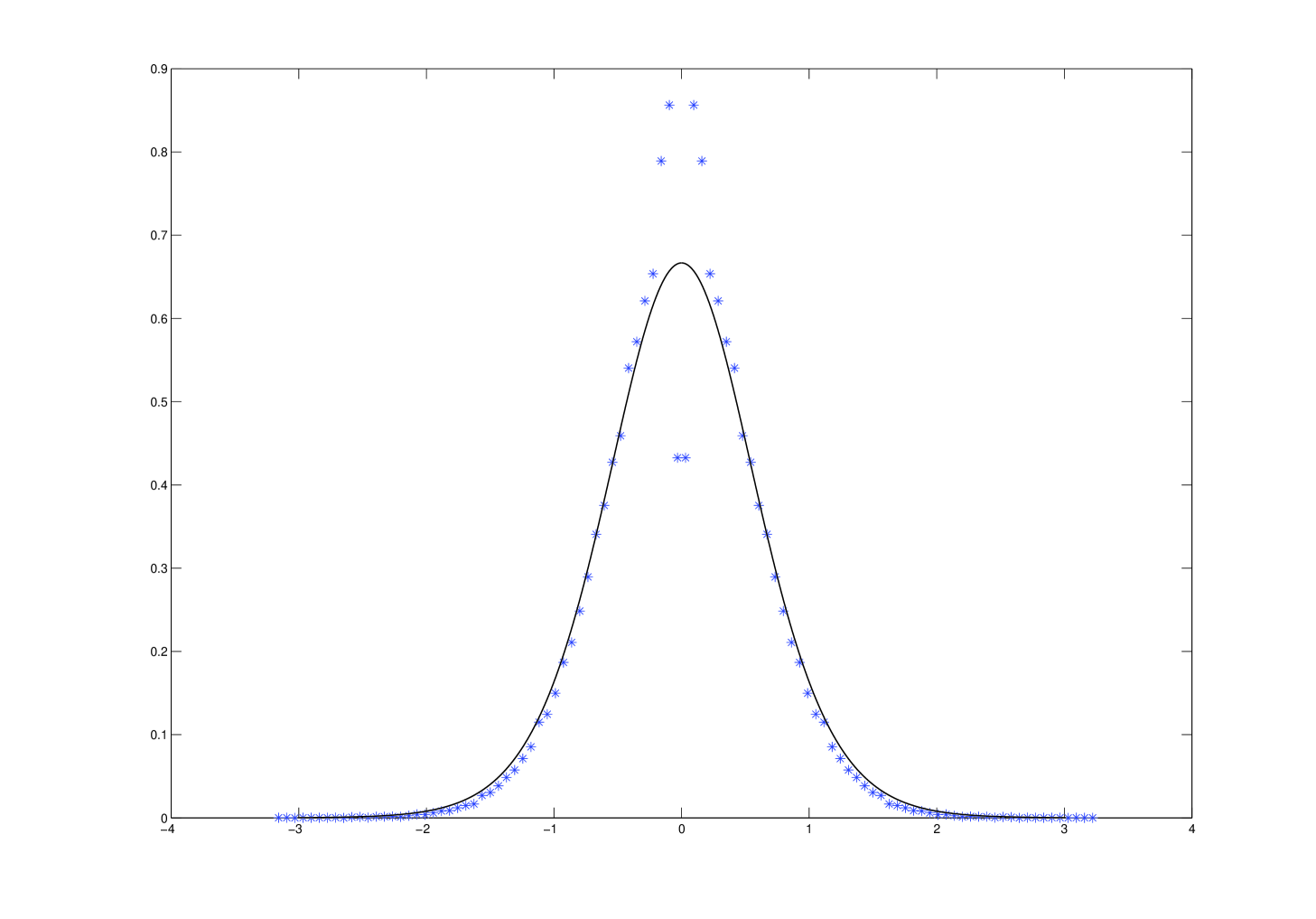
Figure 1: Theoretical curve (solid line) and results of numerical simulations for the profile of the DOS vs. $\eta$. We have used the modified Ablowitz-Ladik diagonalization scheme Weideman and Herbst (1997) to ensure that the determinant of the discretized transfer matrix has unit value. The value of $D$ is $1$, the size of the system is $T=135$ and the step size is $0.075$. The disturbance near $\eta=0$ is a finite-size effect. The localization length grows as $l\sim 3D/2\eta^{2}$ near $\eta=0$ and so numerical results differ from our $T\to\infty$ formula for $|\eta|\lesssim\sqrt{\frac{D}{T}}$.

The localization length $l(\xi,\eta)$ is the inverse of the Lyapunov exponent, $l=\kappa^{-1}$. To see this, we note that the Wronskian of two independent solutions of (4) is constant, therefore if for a given $z$ it has an solution increasing exponentially as $\exp(\kappa t)$, its other solution has to be exponentially decreasing as $\exp(-\kappa t)$. Thus a square integrable solution necessarily decays with length-scale $\kappa^{-1}$ inside the support of $u(t)$. From (41) one can see that states become increasingly delocalized as the eigenvalues approach the real axis on the complex $z$ plane: $l$ diverges as $l\sim\frac{3D}{2\eta^{2}}$ near the real axis. The localization length also determines the stability of the corresponding eigenvalue to the presence of a finite time window of the pulse $T$. Specifically, the typical lifetime of a state with eigenvalue $z$ will scale as $\sim e^{\kappa(\eta)T/2}$ Gredeskul et al. (1990). Indeed we see this in Fig. 1, where for states with localization length comparable to the system length $T$, i.e. close to $\eta=0$, the calculated DOS is no longer valid. To capture the behavior of the DOS in this region, a zero-dimensional analysis similar to Marchetti and Simons (2001); Efetov (1997a, b); Fyodorov and Khoruzhenko and Sommers (1997) is needed.

II.2 Real initial pulse $u(t)$

We can also analyze the opposite case when $u(t)$ is real, Gaussian with $\left\langle u(t)\right\rangle=0$, and $\left\langle u(t)u(t^{\prime})\right\rangle=D\delta(t-t^{\prime})\;$. In this case, the evolution of $w$ and $\phi$ is described by (37) by setting $u_{2}(t)=Im(u(t))=0$. The corresponding steady state solution of the Fokker-Planck equation can be derived from:

$$0 = \partial_{v}\left[(1-v^{2})(\sin^{2}\phi D\partial_{v}-2\eta)\right]P+2\xi\partial_{\phi}P$$

$$- \sin 2\phi\partial_{\phi}\left[\frac{1+v^{2}}{1-v^{2}}+2v\partial_{v}\right]P+\frac{2v^{2}\cos^{2}\phi}{1-v^{2}}\partial_{\phi}^{2}P.$$

For large $|\xi|$, $P$ is independent of $\phi$ to leading order in $\xi$. Therefore the large–$\xi$ expansion is essentially identical to a Fourier expansion. Integrating (II.2) over $\phi$ gives (39). Thus $\tilde{P}$ is to leading order identical to that of the circularly symmetric complex $u$. After some algebra one can derive the next-leading order result. To order $\mathcal{O}(1/\xi^{2})$ the correction to the Lyapunov exponent is

$$\delta\kappa=\frac{D^{2}}{4\xi^{2}}\left(1-\frac{y}{D}\coth\left(\frac{2\eta}{D}\right)+\frac{2\eta^{2}}{D^{2}\sinh^{2}\left(\frac{2\eta}{D}\right)}\right)$$ (44)

resulting in the following correction to the DOS expression of (42)

$$\delta\rho=\frac{D^{2}}{\pi\xi^{2}}\frac{3\eta\coth\left(\frac{2\eta}{D}\right)-\frac{6\eta^{2}}{D\sinh^{2}\left(\frac{2\eta}{D}\right)}-\frac{4\eta^{2}}{D}}{\sinh^{2}\left(\frac{2\eta}{D}\right)}$$ (45)

In the opposite limit of small $\xi$, we expect the distribution in $\phi$ to be peaked. Indeed for $\xi=0$, (II.2) has a solution that is proportional to $\delta(\cos\phi)$. This results in

$$\tilde{P}(v)=\frac{e^{\eta v/D}}{\pi I_{0}(\eta/D)\sqrt{1-v^{2}}}$$ (46)

with corresponding Lyapunov exponent

$$\kappa(\eta)=\frac{\eta I_{1}(\eta/D)}{I_{0}(\eta/D)}$$ (47)

where $I_{0,1}$ are modified Bessel functions of the first kind. We see that compared to (40), (46) is more singular when $|v|\approx 1$, i.e. for large $w$.

III Distribution of $b_{z}$

The complex numbers $b_{z}$, that determine the asymptotics of the bound states of $\bm{U}$, can be expressed in terms of the limiting behavior of the eigenfunctions. Specifically, for $\eta>0$ we have from (17,28)

$$\bm{\Psi}_{z}(t)\rightarrow\left(\begin{array}[]{c}0\\ 1\end{array}\right)e^{izt},\bm{\Psi}_{z}(-t)\rightarrow\left(\begin{array}[]{c}b_{z}^{-1}\\ 0\end{array}\right)e^{izt}\;\mbox{as}\;t\rightarrow\infty$$ (52)

Defining $\tilde{\bm{\Psi}}_{z}(t)\equiv\bm{\Psi}_{z}(-t)$ we can write:

$$b=\lim_{t\to\infty}b(t),\;\;\;b(t)\equiv\frac{\psi_{2}(t)}{\tilde{\psi}_{1}(t)},$$ (53)

where for convenience we have dropped the subscript $z$. The time evolution of $\ln{b}$ is found from (4),

$$\frac{\partial\ln{b}}{\partial t}=i\left(uf+\tilde{u}^{*}\tilde{f}\right)$$ (54)

with $f(t)=\frac{\psi_{1}}{\psi_{2}}$, $\tilde{f}(t)=\frac{\tilde{\psi}_{2}}{\tilde{\psi}_{1}}$, $\tilde{u}(t)\equiv u(-t)$, and

$$\begin{array}[]{l}\frac{\partial f}{\partial t}=-2izf+iu^{*}-iuf^{2}\\ \\ \frac{\partial\tilde{f}}{\partial t}=-2iz\tilde{f}-i\tilde{u}+i\tilde{u}^{*}\tilde{f}^{2}.\end{array}$$ (58)

III.1 Circular complex Gaussian $u(t)$

For a circularly symmetric complex Gaussian $u$, the solution of the Fokker-Planck equation derived from (54,58) relaxes for large times towards a stationary solution where $\ln{b}$ is uniformly distributed , while $f$ and $\tilde{f}$, expressed in polar form, i.e. $f=e^{w+i\phi}$, $\tilde{f}=e^{\tilde{w}+i\tilde{\phi}}$, are distributed independently according to the steady state solution (40). Because of the infinite range of the real part of $\ln{b}$ however, this stationary solution is ill-defined. A better approach is to discretize the size $T$ of the pulse into steps of size $\tau$, equal to the inverse bandwidth of the input signal. Equation (54) then reads

$$\ln{b}=i\tau\sum_{i=1}^{T/2\tau}\left(u_{i}f_{i}+\tilde{u}_{i}^{*}\tilde{f}_{i}\right).$$ (59)

The variables $u_{i},\tilde{u}_{i}$ are i.i.d. Gaussian random variables, distributed according to

$$P_{u}(u)=\frac{1}{\sqrt{2\pi}u_{0}}e^{-\frac{u^{2}}{2u_{0}^{2}}},$$ (60)

where $u_{0}^{2}=D/2\tau$ and $u$ stands for the real or imaginary part of either variable. For large enough $T$, the sum in (59) will be dominated by the domain where the distributions of $f_{i}$ and $\tilde{f}_{i}$ have reached their steady state. In this domain, we find that the real and imaginary parts of the products $x_{i}\equiv u_{i}f_{i}$ and $\tilde{x}_{i}\equiv\tilde{u}_{i}^{*}\tilde{f}_{i}$ have zero mean and the tails of their distributions fall off as the inverse third power of the argument. More precisely,

$$P(\chi)\sim 4\sqrt{\pi}u_{0}^{2}\frac{\eta e^{\frac{2\eta}{D}}}{D\sinh\left(\frac{2\eta}{D}\right)}\frac{1}{|\chi|^{3}}\;,\;\;|\chi|\to\infty$$ (61)

where $\chi$ stands for the real and imaginary parts of $x_{i},\tilde{x}_{i}$. The general theory for sums of random variables Feller (1971); Gnedenko and Kolmogorov (1954); Bouchaud and Georges (1990) then tells us that for large $T/\tau$ the distribution of $\ln|b|$ will be Gaussian, with zero mean and variance

$$\sigma^{2}=4\sqrt{\pi}\frac{\eta e^{\frac{2\eta}{D}}}{\sinh\left(\frac{2\eta}{D}\right)}T\ln\frac{T}{2\tau}.$$ (62)

The imaginary part of $\ln b$ is an angle and so, although it follows the same distribution as the real part, will due to periodicity become uniformly distributed in $[0,2\pi)$. As seen in (28) for $\eta<0$ the corresponding $b_{z}$ is replaced by $-b_{z}^{*}$ AKNS (1974). Thus their distribution will be the same as that of the $b$’s, with $\eta$ replaced by $-\eta$ in (62).

III.2 Real Gaussian $u(t)$

In this case, the Fokker-Planck equation for $\ln b$, derived from (54,58) after setting $u_{2}$ and $\tilde{u}_{2}$ to zero, again predicts that its distribution becomes uniform as the duration $T$ of the pulse grows to infinity. Equation (54) can be written as:

$$\begin{array}[]{lll}\frac{\partial\ln{b}}{\partial t}&=&-\left(ue^{w}\sin{\phi}+\tilde{u}e^{\tilde{w}}\sin{\tilde{\phi}}\right)\\ &&+i\left(ue^{w}\cos{\phi}+\tilde{u}e^{\tilde{w}}\cos{\tilde{\phi}}\right)\end{array}$$ (65)

As seen above, an exact solution to (II.2) is not available, but we can still obtain the first terms of an expansion of the stationary probability distribution in powers of $e^{-w}$:

$$P(w,\phi)\approx\alpha_{1}e^{-w}\delta(\cos{\phi})+\alpha_{2}e^{-2w}+\mathcal{O}\left(e^{-3w}\right)$$ (66)

with an identical expansion for the distribution of $\tilde{w}$ and $\tilde{\phi}$. The constants $\alpha_{1},\alpha_{2}$ depend on $\xi/D$ and $\eta/D$, but, being related to the normalization, they cannot be determined without a knowledge of the full solution. We can thus only partially specify the manner in which the real and imaginary parts of $\ln{b}$ approach uniformity as $T$ grows.

As in the complex case, the real part, $\ln{|b|}$, will be a sum of independent variables $\chi_{i}=u_{i}e^{w_{i}}sin\phi_{i}$. However, in this case, due to the more singular behavior of $P(w,\phi)$ for large $w$, the tails of $\chi_{i}$ will be longer, falling off as $1/|\chi_{i}|^{2}$ for large $T$. As a result, the distribution of $\ln|b|$ will asymptotically follow a Cauchy distribution scaling like $T/\tau$ Gnedenko and Kolmogorov (1954); Bouchaud and Georges (1990). Its statistical median will be zero by symmetry, coming from the even parity of the Gaussian distribution of $u,\tilde{u}$. The phase of $b$ does not get contributions from the first term in (66) because of the delta function in this term. For large $T$, the second term in the expansion dominates, making it uniform over $[0,2\pi)$, in the same manner we saw in the case of complex $u$. Note that for the special case of $\xi=0$, the exact solution (cf. (46)) is proportional to $\delta(\cos\phi)$. The scale parameter of the Cauchy distribution will be

$$\gamma\sim\frac{e^{\eta/D}}{I_{0}(\eta/D)}\frac{T}{\tau}.$$ (67)

Only the transients of the distribution add to the phase of $b$, and numerical simulation shows that they are enough to again make it uniform.

IV Discussion

In the context of the NLSE, the scattering data of the ZS operator uniquely determine the solitonic excitations we get in the optical fiber if we feed one end with a delta-correlated Gaussian signal. Even though the informational contents of the Gaussian signal and its solitonic spectrum are the same, it is easier to consider the effect of amplifier noise in the domain of the scattering data. For example, a small amount of amplifier noise will randomly shift each eigenvalue $z$ by a small amount, while making large changes in the output signal Konotop and Vásquez (1994). The effect of this noise is important to analyze, in order to calculate the ultimate information capacity limits through optical fibers. In principle, to find the capacity one needs to optimize over input signal distributions, which is a formidable task. Instead, in this paper we start with a given input distribution and calculate the corresponding density of states and the corresponding distribution of scattering data $b_{z}$. We leave the analysis of the effects of noise on the spectrum for a future publication.

Appendix A Thouless Formula

The proof of the Thouless formula for the ZS eigenproblem proceeds similarly to the proofs in Thouless (1972); Hayn and John (1987). We consider the system of equations (4) on the interval $[0,T]$. Let $\bm{\Psi}^{l}(t)$,$\bm{\Psi}^{r}(t)$ be two independent solutions of (4) that satisfy the conditions:

$$\bm{\Psi}^{l}(0)=\left(\begin{array}[]{c}\psi^{l}_{1}(0)\\ \psi^{l}_{2}(0)\end{array}\right)\;,\;\;\bm{\Psi}^{r}(T)=\left(\begin{array}[]{c}\psi^{r}_{1}(T)\\ \psi^{r}_{2}(T)\end{array}\right).$$ (72)

We will need to combine this pair of initial and final conditions into a set of boundary conditions for the eigenstates, and for this we let each of them be a one-parameter family of initial(final) conditions to avoid over-determining the problem. This means that $\psi^{l}_{1,2}(0)$ are not chosen independently, but satisfy a single linear relation. The same goes for $\psi^{r}_{1,2}(T)$. The Wronskian of the two solutions, $W=\psi^{r}_{1}\psi^{l}_{2}-\psi^{r}_{2}\psi^{l}_{1}$ is constant. Taking the derivative of (4) with respect to $z$, we obtain an equation for $\partial_{z}\bm{\Psi}^{l}(t)$ whose solution can be written in terms of a matrix Green function $\bm{G}^{l}$:

$$\frac{\partial}{\partial z}\bm{\Psi}^{l}(t)=-\int_{0}^{t}dt^{\prime}\bm{G}^{l}(t,t^{\prime})\bm{\Psi}^{l}(t^{\prime})$$ (73)

with

$$\bm{G}^{l}(t,t^{\prime})=\left\{\begin{array}[]{ll}\frac{i}{W}\left(\bm{\Psi}^{r}(t)\left(\bm{\sigma}_{1}\bm{\Psi}^{l}(t^{\prime})\right)^{T}\right.&\\ \left.\;\;\;\;\;\;\;\;\;-\bm{\Psi}^{l}(t)\left(\bm{\sigma}_{1}\bm{\Psi}^{r}(t^{\prime})\right)^{T}\right)&,\;t>t^{\prime}\\ 0&,\;t<t^{\prime}\end{array}\right.$$ (77)

Here $\bm{\sigma}_{1}=\left(\begin{array}[]{lr}0&1\\ 1&0\end{array}\right)$. The matrix Green function $\bm{G}^{l}$ satisfies the initial conditions

$$\bm{G}^{l}(0,t^{\prime})=0\;,\;\;\left.\frac{\partial}{\partial t}\bm{G}^{l}(t,t^{\prime})\right|_{t=0}=0.$$ (78)

We also define another Green function,

$$\bm{G}(t,t^{\prime})=\left\{\begin{array}[]{l}\frac{i}{W}\bm{\Psi}^{r}(t)\left(\bm{\sigma}_{1}\bm{\Psi}^{l}(t^{\prime})\right)^{T},\;t>t^{\prime}\\ \frac{i}{W}\bm{\Psi}^{l}(t)\left(\bm{\sigma}_{1}\bm{\Psi}^{r}(t^{\prime})\right)^{T},\;t<t^{\prime}\end{array}\right.$$ (81)

which satisfies the conditions (72) (taken together as boundary conditions) and will determine the density of states. The Lyapunov exponent can be expressed as:

$$\kappa=\lim_{T\to\infty}\frac{1}{2T}\left\langle\ln\left({\bm{\psi}^{l}}^{\dagger}(T)\bm{\psi}^{l}(T)\right)\right\rangle.$$ (82)

Before going any further, we must note that the value of $\kappa$ is, with probability one, independent of the initial conditions satisfied by $\bm{\Psi}^{l}$ (the argument is very similar to that for the FGM Bartosch (2001)). To see this, we rewrite the system of equations (4) as:

$$i\frac{\partial}{\partial t}\left(\begin{array}[]{r}\psi_{1}\\ \psi_{2}\end{array}\right)=\bm{V}\left(\begin{array}[]{r}\psi_{1}\\ \psi_{2}\end{array}\right)\;,\;\;\bm{V}=\left(\begin{array}[]{lr}z&-u^{*}\\ -u&-z\end{array}\right).$$ (89)

We can formally write the solution for $\bm{\Psi}^{l}$:

$$\bm{\Psi}^{l}(t)=\bm{S}(t,0)\bm{\Psi}^{l}(0)$$ (90)

$$\bm{S}(t,0)=\mathcal{T}\exp\left[-i\int_{0}^{t}dt^{\prime}\bm{V}(t^{\prime})\right]$$ (91)

where ‘$\mathcal{T}\exp$’ denotes the path-ordered exponential . Because the trace of $\bm{V}$ vanishes, we have $\det{\bm{S}}=1$ Grensing and Grensing (1984). Therefore, if we denote the two eigenvalues of $\bm{S}(t,0)$ by $s_{\pm}(t)$, with $|s_{+}(t)|>|s_{-}(t)|=|s_{+}(t)|^{-1}$, we have

$$\kappa = \lim_{T\to\infty}\frac{1}{2T}\ln\left(|s_{+}(T)\tilde{\psi}_{+}(T)|^{2}+|s_{-}(T)\tilde{\psi}_{-}(T)|^{2}\right)$$ (92)

$$= \lim_{T\to\infty}\frac{1}{T}\ln|s_{+}(T)|,$$

independent of the initial condition, given that the coefficient of the exponentially increasing solution does not vanish, which is the case with probability one in the limit of large $T$.

Now, since ${\bm{\Psi}^{l}}^{\dagger}(T)$ depends only on $z^{*}$ and not on $z$, taking the derivative of (82) with respect to the latter we get

$$\frac{\partial\kappa}{\partial z}=\lim_{T\to\infty}\frac{1}{2T}\left\langle\frac{{\bm{\Psi}^{l}}^{\dagger}(T)\frac{\partial\bm{\Psi}^{l}(T)}{\partial z}}{{\bm{\Psi}^{l}}^{\dagger}(T)\bm{\Psi}^{l}(T)}\right\rangle.$$ (93)

The quantity inside the average can be computed from (73):

$$\frac{{\bm{\Psi}^{l}}^{\dagger}(T)\partial_{z}\bm{\Psi}^{l}(T)}{{\bm{\Psi}^{l}}^{\dagger}(T)\bm{\Psi}^{l}(T)} = -i\frac{{\bm{\Psi}^{l}}^{\dagger}(T)\bm{\Psi}^{r}(T)}{W}\frac{\int_{0}^{T}dt^{\prime}\left(2\psi^{l}_{1}(t^{\prime})\psi^{l}_{2}(t^{\prime})\right)}{{\bm{\Psi}^{l}}^{\dagger}(T)\bm{\Psi}^{l}(T)}$$ (94)

$$+\int_{0}^{T}dt^{\prime}\mbox{Tr}\bm{G}(t^{\prime},t^{\prime})$$

The first term on the right hand side of (94) is almost surely $\mathcal{O}(1)$ in the limit of large $T$ and so does not contribute to the average. We are thus left with

$$\frac{\partial\kappa}{\partial z}=\lim_{T\to\infty}\frac{1}{2T}\left\langle\int_{0}^{T}dt^{\prime}\mbox{Tr}\bm{G}(t^{\prime},t^{\prime})\right\rangle$$ (95)

Taking the derivative of (95) with respect to $z^{*}$ and using the relationFeinberg and Zee (1997) $\rho(z,z^{*})=\frac{1}{\pi T}\frac{\partial}{\partial z^{*}}\left\langle\mbox{Tr}\bm{G}\right\rangle$ we arrive at the Thouless formula for the density of states:

$$\rho(z,z^{*})=\frac{2}{\pi}\frac{\partial^{2}\kappa}{\partial z^{*}\partial z}=\frac{1}{2\pi}\left(\frac{\partial^{2}}{\partial\xi^{2}}+\frac{\partial^{2}}{\partial\eta^{2}}\right)\kappa.$$ (96)

References

- (1)
- Hasegawa and Tappert (1973) A. Hasegawa and F. Tappert, Applied Physics Letters 23, 142 (1973).
- Mollenauer et al. (1980) L. F. Mollenauer, R. H. Stolen, and J. P. Gordon, Phys. Rev. Lett. 45, 1095 (1980).
- Agrawal (1995) G. P. Agrawal, Nonlinear Fiber Optics (Academic Press, San Diego, CA, 1995).
- (5) R.-J. Essiambre and G. P. Agrawal, J. Opt. Soc. Am. B, 14 , no. 2, 314, (1997)
- Zakharov and Shabat (1972) V. E. Zakharov and A. B. Shabat, Sov. Phys. JETP 34, 62 (1972).
- Konotop and Vásquez (1994) V. V. Konotop and L. Vásquez, Nonlinear Random Waves (World Scientific, Singapore, 1994).
- Cover and Thomas (1991) T. M. Cover and J. A. Thomas, Information Theory (John Wiley and Sons, Inc., New York, NY, 1991).
- Gredeskul et al. (1990) S. A. Gredeskul, Y. S. Kivshar, and M. V. Yanovskaya, Phys. Rev. A 41, 3994 (1990).
- Di Francesco et al. (1994) P. Di Francesco et al., Int. J. Mod. Phys. A 9, 4257 (1994).
- Stephanov (1996) M. A. Stephanov, Phys. Rev. Lett. 76, 4472 (1996).
- Forrester and Jancovici (1996) P. J. Forrester and B. Jancovici, Int. J. Mod. Phys. A 11, 941 (1996).
- Feinberg and Zee (1997) J. Feinberg and A. Zee, Nuclear Physics B 504, 579 (1997).
- Miller and Wang (1996) Jonathan Miller and Z. Jane Wang, Phys. Rev. Lett. 76, 1461 (1996).
- Chalker and Wang (1997) J. T. Chalker and Z. Jane Wang, Phys. Rev. Lett. 79, 1797 (1997).
- Janik et al. (1997) R. A. Janik et al., Phys. Rev. E 55, 4100 (1997).
- Janik et al. (1997) R. A. Janik et al., Nuclear Physics B 501, 603 (1997).
- Biane and Lehner (1997) P. Biane and F. Lehner, Colloq. Math. 90, 181 (2001).
- Fyodorov and Sommers (2003) Y. V. Fyodorov and H-J Sommers, J. Phys. A: Math. Gen. 36, 3303 (2003).
- Wiegmann and Zabrodin (2003) P. Wiegmann and A. Zabrodin, J. Phys. A: Math. Gen. 36, 3411 (2003).
- Gudowska-Novak et al. (2003) E. Gudowska-Novak et al., Nuclear Physics B 670, 479 (2003).
- Fyodorov and Khoruzhenko and Sommers (1997) Y. V. Fyodorov, B. A. Khoruzhenko and H-J Sommers, Phys. Lett A 226, 46 (1997).
- Hatano (1998) N. Hatano, Physica A: Statistical Mechanics and its Applications 254, 317 (1998).
- Brézin and Zee (1998) E. Brézin and A. Zee, Nuclear Physics B 509, 599 (1998).
- Goldsheid and Khoruzhenko (1998) I. Y. Goldsheid and B. A. Khoruzhenko, Phys. Rev. Lett. 80, 2897 (1998).
- Thouless (1972) D. J. Thouless, Journal of Physics C: Solid State Physics 5, 77 (1972).
- Goldsheid and Khoruzhenko (2005) I. Y. Goldsheid and B. A. Khoruzhenko, Israel Journal of Mathematics 148, 331 (2005).
- Bartosch (2001) L. Bartosch, Ann. Phys. 10, 799 (2001).
- Ovchinnikov and Erikhman (1977) A. A. Ovchinnikov and N. S. Erikhman, Sov. Phys. JETP 46, 340 (1977).
- Hayn and John (1987) R. Hayn and W. John, Zeitschrift für Physik B 67, 169 (1987).
- Bartosch and Kopietz (1999) L. Bartosch and P. Kopietz, Phys. Rev. B 60, 15488 (1999).
- Mitra and Stark (2001) P. P. Mitra and J. B. Stark, Nature 411, 1027 (2001).
- Green et al. (2002) A. G. Green, P. B. Littlewood, P. P. Mitra, and L. G. L. Wegener, Phys. Rev. E 66, 046627 (2002).
- Turitsyn et al. (2003) K. S. Turitsyn, S. A. Derevyanko, I. V. Yurkevich, and S. K. Turitsyn, Physical Review Letters 91, 203901 (2003).
- Kahn and Ho (2004) J. M. Kahn and K.-P. Ho, IEEE Journal of Selected Topics in Quantum Electronics 10, 259 (2004).
- Halperin (1965) B. I. Halperin, Phys. Rev. 139, A104 (1965).
- Marchetti and Simons (2001) F. M. Marchetti and B. D. Simons, Journal of Physics A: Mathematical and General 34, 10805 (2001).
- Weideman and Herbst (1997) J. A. C. Weideman and B. M. Herbst, Mathematics and Computers in Simulation 43, 77 (1997).
- Efetov (1997a) K. B. Efetov, Phys. Rev. Lett. 79, 491 (1997a).
- Efetov (1997b) K. B. Efetov, Phys. Rev. B 56, 9630 (1997b).
- Feller (1971) W. Feller , An Introduction to Probability Theory, Vols 1 and 2 (Wiley, New York, 1971).
- Gnedenko and Kolmogorov (1954) B. V. Gnedenko and A. N. Kolmogorov, Limit Distributions for Sums of Independent Random Variables (Addison Wesley, Reading, MA, 1954).
- Bouchaud and Georges (1990) J. P. Bouchaud and A. Georges, Physics Reports 195, 127 (1990).
- AKNS (1974) M. J. Ablowitz et al., Studies in Applied Mathematics 53, 249 (1974).
- Grensing and Grensing (1984) D. Grensing and G. Grensing, Phys. Rev. D 30, 2669 (1984).