EUROPEAN ORGANISATION FOR NUCLEAR RESEARCH (CERN)

Measurement of the Cross Section
for open b-Quark Production
in Two-Photon Interactions at LEP

The ALEPH Collaboration

Abstract

Inclusive b-quark production in two-photon collisions has been measured at LEP using an integrated luminosity of $698~{}\mbox{$\mathrm{pb}^{-1}\,$}$ collected by the ALEPH detector with $\sqrt{s}$ between 130 and 209 GeV. The b quarks were identified using lifetime information. The cross section is found to be

$$\mathrm{\sigma(e^{+}e^{-}\rightarrow e^{+}e^{-}b\bar{b}\,X)=(5.4\pm 0.8\,_{stat}\pm 0.8\,_{syst}})\,\mathrm{pb},$$

which is consistent with Next-to-Leading Order QCD.

Submitted to JHEP.

The ALEPH Collaboration

S. Schael

Physikalisches Institut der RWTH-Aachen, D-52056 Aachen, Germany

R. Barate, R. Brunelière, I. De Bonis, D. Decamp, C. Goy, S. Jézéquel, J.-P. Lees, F. Martin, E. Merle, M.-N. Minard, B. Pietrzyk, B. Trocmé

Laboratoire de Physique des Particules (LAPP), IN²P³-CNRS, F-74019 Annecy-le-Vieux Cedex, France

S. Bravo, M.P. Casado, M. Chmeissani, J.M. Crespo, E. Fernandez, M. Fernandez-Bosman, Ll. Garrido,¹⁵ M. Martinez, A. Pacheco, H. Ruiz

Institut de Física d’Altes Energies, Universitat Autònoma de Barcelona, E-08193 Bellaterra (Barcelona), Spain⁷

A. Colaleo, D. Creanza, N. De Filippis, M. de Palma, G. Iaselli, G. Maggi, M. Maggi, S. Nuzzo, A. Ranieri, G. Raso,²⁴ F. Ruggieri, G. Selvaggi, L. Silvestris, P. Tempesta, A. Tricomi,³ G. Zito

Dipartimento di Fisica, INFN Sezione di Bari, I-70126 Bari, Italy

X. Huang, J. Lin, Q. Ouyang, T. Wang, Y. Xie, R. Xu, S. Xue, J. Zhang, L. Zhang, W. Zhao

Institute of High Energy Physics, Academia Sinica, Beijing, The People’s Republic of China⁸

D. Abbaneo, T. Barklow,²⁶ O. Buchmüller,²⁶ M. Cattaneo, B. Clerbaux,²³ H. Drevermann, R.W. Forty, M. Frank, F. Gianotti, J.B. Hansen, J. Harvey, D.E. Hutchcroft,³⁰, P. Janot, B. Jost, M. Kado,² P. Mato, A. Moutoussi, F. Ranjard, L. Rolandi, D. Schlatter, F. Teubert, A. Valassi, I. Videau

European Laboratory for Particle Physics (CERN), CH-1211 Geneva 23, Switzerland

F. Badaud, S. Dessagne, A. Falvard,²⁰ D. Fayolle, P. Gay, J. Jousset, B. Michel, S. Monteil, D. Pallin, J.M. Pascolo, P. Perret

Laboratoire de Physique Corpusculaire, Université Blaise Pascal, IN²P³-CNRS, Clermont-Ferrand, F-63177 Aubière, France

J.D. Hansen, J.R. Hansen, P.H. Hansen, A.C. Kraan, B.S. Nilsson

Niels Bohr Institute, 2100 Copenhagen, DK-Denmark⁹

A. Kyriakis, C. Markou, E. Simopoulou, A. Vayaki, K. Zachariadou

Nuclear Research Center Demokritos (NRCD), GR-15310 Attiki, Greece

A. Blondel,¹² J.-C. Brient, F. Machefert, A. Rougé, H. Videau

Laoratoire Leprince-Ringuet, Ecole Polytechnique, IN²P³-CNRS, F-91128 Palaiseau Cedex, France

V. Ciulli, E. Focardi, G. Parrini

Dipartimento di Fisica, Università di Firenze, INFN Sezione di Firenze, I-50125 Firenze, Italy

A. Antonelli, M. Antonelli, G. Bencivenni, F. Bossi, G. Capon, F. Cerutti, V. Chiarella, P. Laurelli, G. Mannocchi,⁵ G.P. Murtas, L. Passalacqua

Laboratori Nazionali dell’INFN (LNF-INFN), I-00044 Frascati, Italy

J. Kennedy, J.G. Lynch, P. Negus, V. O’Shea, A.S. Thompson

Department of Physics and Astronomy, University of Glasgow, Glasgow G12 8QQ,United Kingdom¹⁰

S. Wasserbaech

Utah Valley State College, Orem, UT 84058, U.S.A.

R. Cavanaugh,⁴ S. Dhamotharan,²¹ C. Geweniger, P. Hanke, V. Hepp, E.E. Kluge, A. Putzer, H. Stenzel, K. Tittel, M. Wunsch¹⁹

Kirchhoff-Institut für Physik, Universität Heidelberg, D-69120 Heidelberg, Germany¹⁶

R. Beuselinck, W. Cameron, G. Davies, P.J. Dornan, M. Girone,¹ N. Marinelli, J. Nowell, S.A. Rutherford, J.K. Sedgbeer, J.C. Thompson,¹⁴ R. White

Department of Physics, Imperial College, London SW7 2BZ, United Kingdom¹⁰

V.M. Ghete, P. Girtler, E. Kneringer, D. Kuhn, G. Rudolph

Institut für Experimentalphysik, Universität Innsbruck, A-6020 Innsbruck, Austria¹⁸

E. Bouhova-Thacker, C.K. Bowdery, D.P. Clarke, G. Ellis, A.J. Finch, F. Foster, G. Hughes, R.W.L. Jones, M.R. Pearson, N.A. Robertson, T. Sloan, M. Smizanska

Department of Physics, University of Lancaster, Lancaster LA1 4YB, United Kingdom¹⁰

O. van der Aa, C. Delaere,²⁸ G.Leibenguth,³¹ V. Lemaitre²⁹

Institut de Physique Nucléaire, Département de Physique, Université Catholique de Louvain, 1348 Louvain-la-Neuve, Belgium

U. Blumenschein, F. Hölldorfer, K. Jakobs, F. Kayser, A.-S. Müller, B. Renk, H.-G. Sander, S. Schmeling, H. Wachsmuth, C. Zeitnitz, T. Ziegler

Institut für Physik, Universität Mainz, D-55099 Mainz, Germany¹⁶

A. Bonissent, P. Coyle, C. Curtil, A. Ealet, D. Fouchez, P. Payre, A. Tilquin

Centre de Physique des Particules de Marseille, Univ Méditerranée, IN²P³-CNRS, F-13288 Marseille, France

F. Ragusa

Dipartimento di Fisica, Università di Milano e INFN Sezione di Milano, I-20133 Milano, Italy.

A. David, H. Dietl,³² G. Ganis,²⁷ K. Hüttmann, G. Lütjens, W. Männer³², H.-G. Moser, R. Settles, M. Villegas, G. Wolf

Max-Planck-Institut für Physik, Werner-Heisenberg-Institut, D-80805 München, Germany

J. Boucrot, O. Callot, M. Davier, L. Duflot, J.-F. Grivaz, Ph. Heusse, A. Jacholkowska,⁶ L. Serin, J.-J. Veillet

Laboratoire de l’Accélérateur Linéaire, Université de Paris-Sud, IN²P³-CNRS, F-91898 Orsay Cedex, France

P. Azzurri, G. Bagliesi, T. Boccali, L. Foà, A. Giammanco, A. Giassi, F. Ligabue, A. Messineo, F. Palla, G. Sanguinetti, A. Sciabà, G. Sguazzoni, P. Spagnolo, R. Tenchini, A. Venturi, P.G. Verdini

Dipartimento di Fisica dell’Università, INFN Sezione di Pisa, e Scuola Normale Superiore, I-56010 Pisa, Italy

O. Awunor, G.A. Blair, G. Cowan, A. Garcia-Bellido, M.G. Green, T. Medcalf,²⁵ A. Misiejuk, J.A. Strong,²⁵ P. Teixeira-Dias

Department of Physics, Royal Holloway & Bedford New College, University of London, Egham, Surrey TW20 OEX, United Kingdom¹⁰

R.W. Clifft, T.R. Edgecock, P.R. Norton, I.R. Tomalin, J.J. Ward

Particle Physics Dept., Rutherford Appleton Laboratory, Chilton, Didcot, Oxon OX11 OQX, United Kingdom¹⁰

B. Bloch-Devaux, D. Boumediene, P. Colas, B. Fabbro, E. Lançon, M.-C. Lemaire, E. Locci, P. Perez, J. Rander, B. Tuchming, B. Vallage

CEA, DAPNIA/Service de Physique des Particules, CE-Saclay, F-91191 Gif-sur-Yvette Cedex, France¹⁷

A.M. Litke, G. Taylor

Institute for Particle Physics, University of California at Santa Cruz, Santa Cruz, CA 95064, USA²²

C.N. Booth, S. Cartwright, F. Combley,²⁵ P.N. Hodgson, M. Lehto, L.F. Thompson

Department of Physics, University of Sheffield, Sheffield S3 7RH, United Kingdom¹⁰

A. Böhrer, S. Brandt, C. Grupen, J. Hess, A. Ngac, G. Prange

Fachbereich Physik, Universität Siegen, D-57068 Siegen, Germany¹⁶

C. Borean, G. Giannini

Dipartimento di Fisica, Università di Trieste e INFN Sezione di Trieste, I-34127 Trieste, Italy

H. He, J. Putz, J. Rothberg

Experimental Elementary Particle Physics, University of Washington, Seattle, WA 98195 U.S.A.

S.R. Armstrong, K. Berkelman, K. Cranmer, D.P.S. Ferguson, Y. Gao,¹³ S. González, O.J. Hayes, H. Hu, S. Jin, J. Kile, P.A. McNamara III, J. Nielsen, Y.B. Pan, J.H. von Wimmersperg-Toeller, W. Wiedenmann, J. Wu, Sau Lan Wu, X. Wu, G. Zobernig

Department of Physics, University of Wisconsin, Madison, WI 53706, USA¹¹

G. Dissertori

Institute for Particle Physics, ETH Hönggerberg, 8093 Zürich, Switzerland.

1 Introduction

The cross section for heavy flavour production in two-photon interactions is expected to be reliably calculated in perturbative QCD, particularly in the case of b-quark production, as the heavy quark mass introduces a relatively large scale into the process. The cross section has been calculated in Next-to-Leading Order (NLO) QCD to be between 2.1 and 4.5 pb [1], which is two orders of magnitude smaller than that for charm production, which in turn is approximately 6% of the total cross section for hadron production. The latter is dominated by soft processes involving u, d and s quarks. The process of heavy flavour production in two-photon interactions at LEP energies is dominated by the two classes of diagrams shown in Fig. 1. These are referred to as the ‘direct’ process in which the photon couples directly to the heavy quark, and the ‘single resolved’ process in which one photon first fluctuates into quarks and gluons. This separation is unambiguous up to next-to-leading order due to the heavy quark mass [2]. In the resolved diagram the dominant process is photon-gluon fusion where a gluon from the resolved photon couples with the heavy quark. Heavy quark production via double resolved processes is highly suppressed at LEP energies [1].

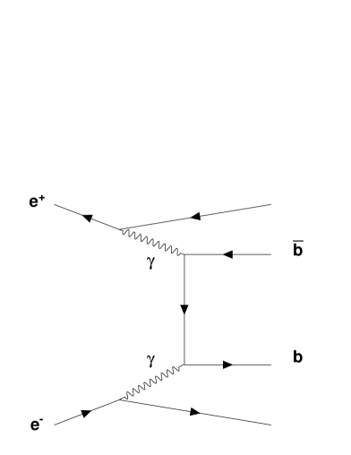
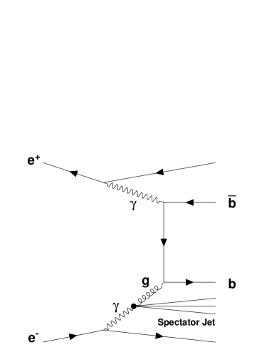
Direct	Single Resolved

Figure 1: Diagrams contributing to b-quark production in $\gamma\gamma$ collisions.

The only measurement of b-quark production in two-photon collisions published to date is by the L3 Collaboration, obtained from a fit to the transverse momentum of leptons with respect to jets [3]: the cross section was measured to be about three times the prediction of NLO QCD. Similar results have been reported at conferences by OPAL [4] and DELPHI [5].

This paper presents a measurement of open b-quark production in data collected between 1996 and 2000 with an integrated luminosity of $698~{}\mbox{$\mathrm{pb}^{-1}\,$}$. During this period the LEP centre of mass energy ranged from 130 to 209 GeV, with a mean of 196 GeV. The result is the first published measurement in which lifetime information has been used to identify heavy flavour quarks in two-photon physics. The paper is organised as follows. Section 2 gives a brief description of the ALEPH detector, Section 3 presents the event generators used for the simulation of the signal and backgrounds, Section 4 describes the jet finding procedure employed, and Section 5 describes the b tagging procedure. The initial event selection based on cuts is described in Section 6, followed in Section 7 by the final selection which uses an event weighting procedure. In Section 8 the efficiency calculation is described, with the resulting cross Section given in Section 9. In Section 10 the calculation of the systematic uncertainties is described, and in Section 11 a number of cross checks are presented. Finally in Section 12 the final value for the cross section of open b-quark production is shown.

2 ALEPH Detector

The ALEPH detector has been described in detail elsewhere [6]. Critical to this analysis is the ability to accurately measure charged particles. These are detected in a large time projection chamber (TPC) supplemented by information from the inner tracking chamber (ITC) which is a cylindrical drift chamber sitting inside the TPC, and a two-layer silicon strip vertex detector (VDET) which surrounds the beam pipe close to the interaction point. The VDET was upgraded in 1996 for the high energy running of LEP. It consists of 48 modules of double sided silicon strip detectors arranged in two concentric cylinders. The resolution in $r\phi$ is $10\,\mu{\rm m}$, while that in $z$ rises from $15\,\mu{\rm m}$ for tracks perpendicular to the beam direction to 50 $\mu\mathrm{m}$ for tracks at $\cos{\theta}=0.85$ [7]. Charged particle transverse momenta are measured with a resolution of $\delta p_{\mathrm{t}}/p_{\mathrm{t}}=6\times 10^{-4}p_{\mathrm{t}}\oplus 0.005$ ($p_{\mathrm{t}}$ in $\mathrm{GeV}/c$).

Outside the TPC lies the electromagnetic calorimeter (ECAL) whose primary purpose is the identification and measurement of electromagnetic clusters produced by photons and electrons. It is a lead/proportional-tube sampling calorimeter segmented in $0.9^{\circ}\times 0.9^{\circ}$ projective towers read out in three sections in depth. It has a total thickness of 22 radiation lengths and a relative energy resolution of $0.18/\sqrt{E}\oplus 0.009$, ($E$ in GeV) for photons. Outside the ECAL, a superconducting solenoidal coil produces a $1.5\,{\rm T}$ axial magnetic field and the iron return yoke for the magnet is instrumented with 23 layers of streamer tubes to form the hadron calorimeter (HCAL). The HCAL has a relative energy resolution for hadrons of $0.85/\sqrt{E}$ ($E$ in GeV). The outermost detector of ALEPH is a set of muon chambers which consist of two double-layers of streamer tubes. Near the beam pipe, $3\,{\rm m}$ from the interaction point on either side, are two luminosity calorimeters, the LCAL and SiCAL, which are electromagnetic calorimeters specifically designed to measure the luminosity via Bhabha scattering.

The information from the tracking detectors and the calorimeters are combined in an energy flow algorithm [6]. For each event, the algorithm provides a set of charged and neutral reconstructed particles, called energy-flow objects.

3 Monte Carlo Simulation

The PYTHIA [8] Monte Carlo program was used to simulate the two-photon processes. The production of b and c quarks by the direct and resolved process was modelled separately using PYTHIA 6.1 with matrix elements including mass effects. For the resolved process the photon’s parton distribution function was the PYTHIA default (SaS 1D) [9].

The charm quark production cross section was normalised using the average of the measurements made at LEP2, $\sigma(\mathrm{e^{+}e^{-}\rightarrow e^{+}e^{-}c\bar{c}\,X)=930\pm 120\,{\rm pb}}$ [3, 10]. All remaining hadron production by two-photon collisions was simulated using the standard PYTHIA machinery for incoming photon beams [11]. The result of this paper will be compared to a calculation which is valid for real photons ($Q_{\gamma}^{2}\approx 0$) so events with $Q_{\gamma}^{2}>6$ were treated as a background and will be referred to as $\gamma^{*}\gamma\,$events for the remainder of this paper. The background from $\mathrm{e^{+}e^{-}\rightarrow q\bar{q}}$ was produced using the KK Monte Carlo program [12].

4 Jet Finding

The direction of partons in an event was estimated using jets found with a dedicated jet finder (PTCLUS) that optimises the reconstruction of resolved events. The PTCLUS algorithm consists of three steps.

• The most energetic energy flow object is taken as the first jet initiator. The algorithm then loops through all the remaining objects in order of decreasing energy. If the angle between an object’s momentum vector ${\it p}$ and the jet momentum $p_{\mbox{\unboldmath$\mathrm{jet}$}}$ is less than $90^{\circ}\,$and the transverse momentum of the object with respect to $p+p_{\mbox{\unboldmath$\mathrm{jet}$}}\,\,$is smaller than 0.5 $\mathrm{GeV}/c$ then, the object is added to the jet. Otherwise the object is used as a new jet initiator. The procedure is repeated until all objects have been assigned to a jet.

• The distance between two jets is defined as $Y=M^{2}/E^{2}_{\mathrm{vis}}$ where $M$ is the invariant mass of the pair of jets, assumed to be massless, and $E_{\mathrm{vis}}$ is the visible energy. The pair of jets with the smallest value of $Y$ is merged provided $Y<0.1$ and they are within $90^{\circ}$ of each other.

• The process of merging jets may result in objects having a larger transverse momentum with respect to the jet to which they have been assigned than to another jet. If this is the case the object is reassigned to the other jet. A maximum of five reassignments may occur after each merger.

The last two steps are repeated until no pair of jets has $Y<0.1$.

5 b Tagging

This analysis relies on the ALEPH b tagging software developed to identify b quarks via their long lifetimes [13]. It identifies charged tracks that appear to originate from a point away from the primary event vertex, and along the direction of the reconstructed b quark. The b tagging algorithm relies on the impact parameter of charged tracks to indicate the presence of long lived particles. The impact parameter is defined as the distance of closest approach in space between a track and the main vertex in the event. It is signed positive (negative) if the point of closest approach between the track and the estimated b hadron flight path is in front of (behind) the main vertex, along the direction of the b momentum estimated using the jets found by PTCLUS. The impact parameter significance $S$ is defined as the signed impact parameter divided by its estimated measurement error. A fit to the negative $S$ distribution is used to derive a function which when applied to a single track can be used to obtain $P_{\mathrm{track}}$, the probability that a track originated at the main event vertex. Only tracks which are likely to have $S$ reliably measured are used, in particular they are required to have at least one associated VDET hit. The primary vertex in an event is found using a procedure specifically designed for use in b tagging. Probabilities from tracks with positive $S$ are combined to form tagging variables. Three tagging variables are used in this analysis. These are $P_{\mathrm{event}}$,$P_{\mathrm{jet1}}$, and $P_{\mathrm{jet2}}$ which are respectively the probabilities that the whole event, the first jet or the second jet contained no decay products from long lived particles.

6 Event Selection

The preselection stage of the analysis identified events which were predominantly from low $Q_{\gamma}^{2}$ two-photon interactions. Events were required to have

• at least 5 charged tracks;

• invariant mass of all energy flow objects ($W_{\mathrm{vis}}$) between 4 and 40 $\mathrm{GeV/}c^{2}$ ;

• total energy in the luminosity calorimeters SiCAL and LCAL less than 30 GeV;

• total transverse momentum of the event, relative to the beam direction, less than 6 $\mathrm{GeV}/c$;

• thrust less than 0.97.

The PTCLUS algorithm was used to find jets using all energy flow objects with $|\cos\theta|$ less than 0.94. This cut results in the b quark jets having similar properties in direct and resolved events. Between 1 and 3 jets were found and ranked by how close their mass was to the nominal b quark mass of 5 $\mathrm{GeV/}c^{2}$ , with Jet 1 being the closest, Jet 2 the next closest, etc. After the preselection approximately 80% of the Jet 1 sample were within $15^{\circ}$ of a parton in the direct $\mathrm{\gamma\gamma\rightarrow b\bar{b}}$ Monte Carlo, while the corresponding figure for the resolved Monte Carlo was $70\%$.

Figure 2: Distribution of $W_{\mathrm{vis}}$  and the energy of Jet 1 in data and simulation after preselection.

From the distribution of $W_{\mathrm{vis}}$, and the energy of Jet 1 shown in Fig. 2 it can be seen that the preselected sample is dominated by events containing light quarks.

A further selection was applied to enhance the fraction of events from the signal process, $\mathrm{\gamma\gamma\rightarrow b\bar{b}\,X}$. Events were required to have

• at least 7 charged tracks;

• invariant mass of all energy flow objects between 8 and 40 $\mathrm{GeV/}c^{2}$ ;

• at least two jets;

• $P_{\mathrm{event}}<0.05$;

• the third largest impact parameter significance $S$ greater than 0.0;

• the fourth largest impact parameter significance $S$ greater than -10.

Figure 3 shows the distribution of $W_{\mathrm{vis}}$, and the energy of Jet 1 for events at this stage of the analysis. Comparison with Fig. 2 shows that while the proportion of the events in this sample originating from b quarks has increased compared to the preselection, the dominant source of events is still $\mathrm{\gamma\gamma\rightarrow uds}$ and $\mathrm{\gamma\gamma\rightarrow c\bar{c}\,X}$.

Figure 3: Distribution of $W_{\mathrm{vis}}$  and the energy of Jet 1 in data and simulation after selection.

7 Iterative Discriminant Analysis

In this analysis the likelihood that an event belongs either to the signal or to the background is determined by means of an Iterative Discriminant Analysis (IDA) [14]. The details of the method are described in the Appendix. The method generalises standard linear discriminant analysis and proceeds through a series of iterations. At each iteration $i$ events are selected by applying a cut on the discriminant function for that iteration ($D_{i}$) and a new discriminant function is then generated for the remaining events. The simulated samples described in section 3 were used to determine the IDA coefficients. A set of 11 variables was chosen as input to the IDA process, these were:

• $P_{\mathrm{event}}$,$P_{\mathrm{jet1}}$,$P_{\mathrm{jet2}}$;

• mass and transverse momentum of Jet 1;

• the five highest track impact parameter significances $S$ seen in the event;

• the thrust of the event.

After each IDA iteration the simulations of signal and background were used to choose whether to perform another iteration, and where to place the cut on $D_{i}$. A series of possible values at which to apply a selection on $D_{i}$ were chosen starting with one that selects 100% of the signal and increasing in steps of 1% until no signal remained. At each step the significance of the expected signal above the cut was calculated by dividing it by the predicted error for the integrated luminosity in the data, including estimated statistical and systematic uncertainties. Having determined the value of $D_{i}$ at which the significance was maximal, the cut to be applied to the discriminant variable $D_{i}$ was set at a value $\Delta_{\mathnormal{D}}$ lower. The value of $\Delta_{\mathnormal{D}}$ was set to 1.5 for the first iteration, and halved at each subsequent iteration. This continued for three iterations after which there was no further improvement in the predicted significance.

The coefficients of the discriminant analysis and and cut values derived from this procedure were then applied to the data. However in order to perform various systematic checks which will be described later, it proved necessary to loosen the cut on $D_{2}$. This had no significant impact on the purity of the signal obtained. The final cut on $D_{3}$  was chosen to maximise the size of the signal relative to its uncertainty (both statistical and systematic). Table 1 shows the fraction of the total event sample estimated to come from various sources and the number of events in the data, at different stages in the analysis. The distribution of the discriminant variables $D_{i}$ in the data and simulation is shown in Fig. 4 for each iteration of the IDA process.

The final selection yielded 93 events in the data. The background was calculated using separate samples of simulated events from those used to tune the IDA parameters. It was found to consist of 18.8 events from $\mathrm{\gamma\gamma\rightarrow c\bar{c}\,X}$, 3.9 events from $\gamma^{*}\gamma\rightarrow\,X$ and 1.5 events from $\mathrm{e^{+}e^{-}}$ annihilation.

	Cross sect-	Analysis stage
Sample	ion (pb)	1	2	3	4	5
$\mathrm{\gamma\gamma\rightarrow uds}$	16000	89	73	12	9	0
$\mathrm{\gamma\gamma\rightarrow c\bar{c}}\,X$	930	10	25	40	35	23
$\gamma^{*}\gamma\rightarrow X$	84	0	1	4	5	5
$\mathrm{e^{+}e^{-}\rightarrow q\bar{q}}$	83	0	0	2	2	2
$\mathrm{\gamma\gamma\rightarrow b\bar{b}}\,X$	4	0	1	41	50	70
data	-	2696021	16810	244	197	93

Table 1: Summary of the analysis. The first 5 rows show the cross section used for the simulation and the fraction (%) of each simulated subset at progressive stages of the analysis. The final row shows the number of events remaining in the data at each stage. The numeric column labels denote the analysis stages, they are (1) pre selection, (2) selection, (3) IDA iteration 1, (4) IDA iteration 2, (5) final cut on $D_{3}$.

 

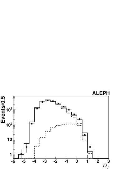
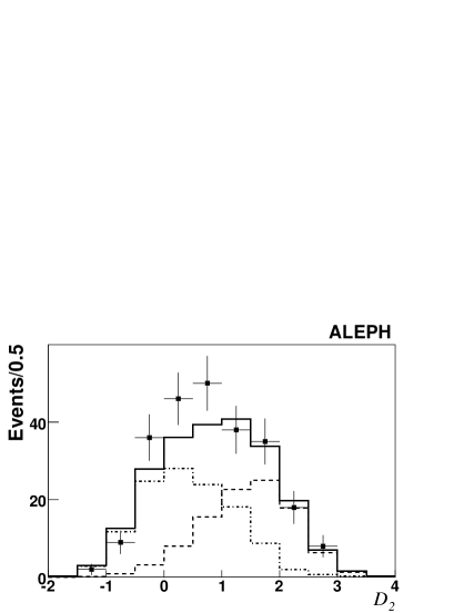
Figure 4: Distributions of the discriminant variable in data and Monte Carlo samples after each iteration of the IDA process. The points with error bars are the data, the dashed histogram is the simulated signal, the dash-dot histogram is the simulated background, and the solid histogram is the sum of signal and background simulations. Each distribution has been translated along the horizontal axis so that the selection cut is at zero. The signal simulation has been weighted according to the fit described in Section 8.

8 Efficiency Calculation

The efficiency for signal events to pass the selection procedure was estimated using a separate sample of simulated signal events to that used to determine the IDA parameters. The efficiency is different for the direct and resolved components so in order to calculate the total efficiency, the relative size of the two components must be determined. This was found from the data by performing a fit to the $x_{\gamma}^{\mathrm{min}}\,$distribution in the data after subtracting the background. The variable $x_{\gamma}^{\mathrm{min}}\,$is defined as the smallest of $x_{\gamma}^{+}$ and $x_{\gamma}^{-}$ where

$$x_{\gamma}^{\pm}=\frac{\sum_{i=1,2}(E^{i}\pm p_{z}^{i})}{(E^{\mathrm{tot}}\pm p_{z}^{\mathrm{tot}})}.$$ (1)

Here $E^{i}$, $p_{z}^{i}$ are the energy and longitudinal momentum of jet $i$, while $E^{\mathrm{tot}}$ and $p_{z}^{\mathrm{tot}}$ are the energy and longitudinal momentum of the whole event. The sum is calculated for the highest and second highest energy jets in the event. The $x_{\gamma}^{\pm}$ variables are used in two-photon and photoproduction experiments to distinguish direct and resolved events. They represent the fraction of the incoming photon’s four-momentum that has gone into the hard scattering process. For perfectly measured events the value of $x_{\gamma}$ is identically 1 for direct photons, and less than 1 for resolved photons, as in the latter case some of the photon’s four momentum is taken away by the spectator jet. In practice direct events are characterised by having both $x^{+}$ and $x^{-}$ larger than 0.75, while single resolved events tend to have either $x^{+}$ or $x^{-}$ less than 0.75, and double resolved events have both values less than 0.75 [15]. In this analysis only direct and single resolved processes need be considered so $x_{\gamma}^{\mathrm{min}}\,$can be used to separate them experimentally.

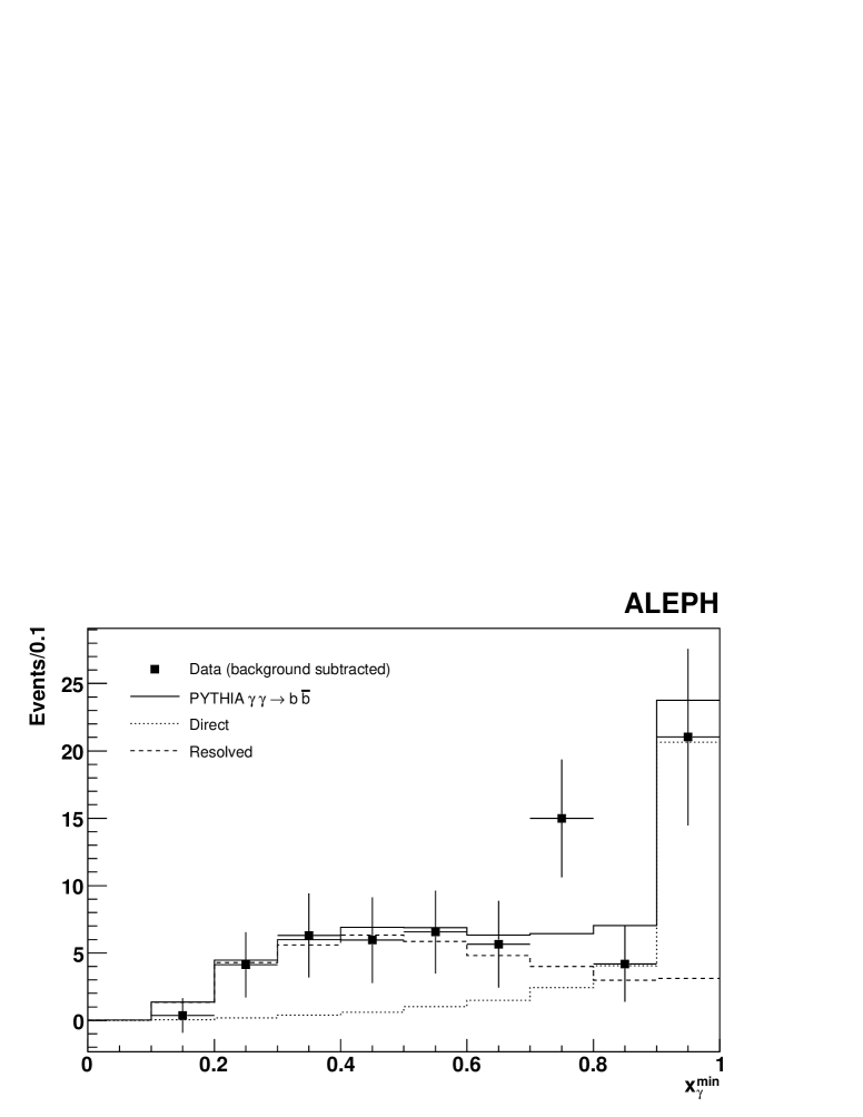
Figure 5: The $x_{\gamma}^{\mathrm{min}}\,$distribution. The points with error bars are the data after subtracting the background. The histograms show the distribution in the simulated direct and resolved signal after fitting to the data.

The $x_{\gamma}^{\mathrm{min}}\,$distribution is shown in Fig. 5 for data after subtracting background and the simulated direct and resolved components after fitting to the data. The result of the fit is that there are $30.8\pm 11.3$ direct and $38.3\pm 11.9$ resolved events in the data. The efficiencies are $0.022$ for the direct term, and $0.016$ for the resolved term. The mean efficiency is calculated to be $0.0184\pm 0.0009$ where the error comes from the fit to the fraction of direct and resolved events. The trigger efficiency for events passing the final cut has been measured using independent triggers and found to be negligibly less than 100%.

9 Cross Section Calculation

The total cross section is calculated as

$$\sigma(\mathrm{e^{+}e^{-}\rightarrow e^{+}e^{-}b\bar{b}\,X})=\frac{N-b}{\epsilon\mathcal{L}}$$ (2)

where $N$ is the number of events observed, $b$ is the estimated background, $\epsilon$ is the efficiency and $\mathcal{L}$ is the luminosity. With $N=93$, $b=24.2$, $\epsilon=0.0184$ and $\mathcal{L}=698~{}\,{\rm pb}^{-1}\,$ the result is $\sigma(\mathrm{e^{+}e^{-}\rightarrow e^{+}e^{-}b\bar{b}\,X})=(5.4\pm 0.8)\,{\rm pb}$ where the error is statistical only.

10 Systematic Uncertainties

10.1 Background Estimate

The uncertainty on the background derives from the uncertainty on the cross section for each component. This is estimated to be 12.5% for $\mathrm{\gamma\gamma\rightarrow c\bar{c}\,X}$ [10], 40% for $\gamma^{*}\gamma\rightarrow X$ [16] and 3% for $\mathrm{e^{+}e^{-}\rightarrow q\bar{q}}$ [17]. The resulting uncertainty on the background is $2.8$ events.

10.2 Monte Carlo Simulation

To assess the sensitivity of the efficiency to the modelling of the physics channels a second sample of signal events was generated using the HERWIG program [18] (version 6.201). The difference in efficiency obtained using these events was 8.6%, and this has been used as a systematic error. The effect of varying the b-quark fragmentation function in the simulation was checked and found to be negligible.

10.3 $W_{\mathrm{vis}}$ dependence

Figure 3 shows some discrepancy in the $W_{\mathrm{vis}}$  distribution at the highest values. To check whether this had any influence on the final result the analysis was repeated with the maximum accepted $W_{\mathrm{vis}}$ set to 30 $\mathrm{GeV/}c^{2}$ . This resulted in the measured cross section dropping by 0.5 pb. This has been included as a conservative systematic error.

11 Cross Checks of the Analysis

11.1 Stability with respect to the $D_{3}$ cut

An important check of the analysis comes from the dependence of the result on the $D_{3}$ cut. In Fig. 6 the cross section measurements obtained when varying the $D_{3}$ cut either side of the chosen value are plotted along with the uncorrelated errors of each point with respect to the point at the chosen cut. No systematic trend is observed. Similar studies on the $D_{1}$ and $D_{2}$ cuts did not reveal significant effects so no additional systematic error was assigned.

Figure 6: Stability of the cross section measurement with respect to changing the cut on $D_{3}$. The total error is shown at the chosen cut value ($\mathnormal{D}_{3}=0$), while for the other points the uncertainties relate to the difference of each point with respect to the chosen cut. The bins are defined such that each contains 10 more data events than that to its right.

11.2 $W_{\mathrm{vis}}$ distribution

An independent test of the fit to direct and resolved components is given by the distribution of $W_{\mathrm{vis}}$  which is shown in Fig. 7. The direct and resolved components also have a significantly different distribution in this variable and together they give a good description of the data.

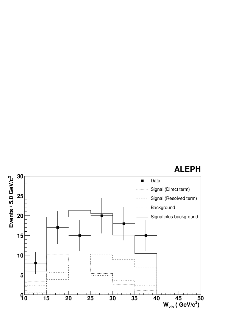
Figure 7: The distribution of $W_{\mathrm{vis}}$  in selected $\mathrm{\gamma\gamma\rightarrow b\bar{b}\,X}$ data. Points with error bars are the data. The histograms show the distribution in the background, the direct and resolved signal and the sum of signal plus background.

11.3 Semileptonic decays

Approximately 20% of b quarks undergo semileptonic decays, in which an electron or a muon is generated from the W; therefore about 14 electrons and 14 muons are expected to be produced, on average, in the observed signal sample of 74 $\mathrm{b\bar{b}}$ events, through direct semileptonic decays. Because of the large mass of the b quark, the leptons tend to be at higher transverse momentum relative to the accompanying jet than those from the decay of the lighter quarks. The production of leptons from semileptonic decays of the secondary charm in the b decay chain is also sizeable, but the selection efficiency is considerably smaller because of the softer momentum and transverse momentum spectra. All charged tracks with momentum greater than 2 $\mathrm{GeV}/c$  were considered as candidate electrons or muons.

Muons were identified from the pattern of energy deposition left in the HCAL. In addition candidate muon tracks were required not be part of a track showing evidence of a kink in the TPC, to have at least 5 hits in the ITC, and have a $\mathrm{d}E/\mathrm{d}x$ measurement in the TPC consistent with the expectation for a muon.

Electrons were required to have a cluster in the ECAL whose transverse and longitudinal shape was consistent with that expected for an electromagnetic shower, and whose energy was consistent with the momentum measured in the TPC. In addition they were required to have at least one VDET hit and at least 3 ITC hits and not be from an identified converted photon.

Simulation studies show that the majority of misidentified leptons or leptons not originating from the decay of b hadrons are found at low transverse momentum relative to the nearest jet. Requiring the lepton transverse momentum to be greater than 1 $\mathrm{GeV}/c$  relative to the nearest jet leaves 0.1% of misidentified leptons and 2.5% from sources other than b hadron decays.

Figure 8 shows the distribution of transverse momentum of electrons and muons with respect to the nearest jet in the final sample of events. If the lepton is included in the jet then its momentum has been subtracted from the jet before calculating the transverse momentum. The signal of 6 leptons is consistent with the prediction of 6 from the signal simulation plus 0.9 from the background.

Figure 8: The transverse momentum of electrons and muons with respect to the nearest jet in selected $\mathrm{\gamma\gamma\rightarrow b\bar{b}\,X}$ data. Points with error bars are the data. The histograms show the distribution in the background, the direct and resolved signal and the sum of signal plus background.

12 Conclusions

The cross section for the process $\mathrm{e^{+}e^{-}\rightarrow e^{+}e^{-}b\bar{b}\,X}$ has been measured to be

$$\mathrm{\sigma(e^{+}e^{-}\rightarrow e^{+}e^{-}b\bar{b}\,X)=(5.4\pm 0.8\,_{stat}\pm 0.8\,_{syst})\,pb}$$

which is consistent with the prediction of NLO QCD [1] of between 2.1 and 4.5 pb but barely consistent with the result quoted by the L3 Collaboration [3], $\mathrm{(12.8\pm 1.7_{stat}\pm 2.3_{syst}\,)}\,\mathrm{pb}$.

Appendix A Iterative Discriminant Analysis

Discriminant analysis is a technique for classifying a set of observations into predefined classes. The purpose is to determine the class of an observation based on a set of input variables. The model is built based on a set of observations for which the classes are known. In standard discriminant analysis a set of linear functions of the variables, known as discriminant functions, are constructed, such that $L=\sum_{i=1,n}(b_{i}x_{i})+c$ , where the $b$’s are discriminant coefficients, the $x_{i}$ are the $n$ input variables and $c$ is a constant. In the method known as Iterative Discriminant Analysis [14] (IDA) the vector of input variables $\mathbf{x}$ is extended to include all their products $x_{i}x_{j}$ ( $i\neq j$). In addition the process is repeated a number of times with a selection being applied at each iteration and a new discriminant calculated. In detail the IDA procedure works as follows:

• For each event fill a vector $\mathbf{y}$ containing the n variables and $(n^{2}-n)/2$ products of those variables.

• Calculate the variance matrix $\mathbf{V}=\mathbf{V}_{\mathrm{s}}+\mathbf{V}_{\mathrm{b}}$, where $\mathbf{V}_{\mathrm{s}}$ is the variance matrix of the signal and $\mathbf{V}_{\mathrm{b}}$ is the variance matrix of the background; $\mathbf{V}_{\mathrm{s}}$ and $\mathbf{V}_{\mathrm{b}}$ are weighted so that they have equal importance.

• Calculate $\mathbf{\Delta}\mu$, the difference in the means of the signal and background, for each element of $\mathbf{y}$.

• Invert the variance matrix $\mathbf{V}$ and multiply by $\mathbf{\Delta}\mu$, to obtain the vector of coefficients $\mathbf{a}=\mathbf{V}^{-1}\mathbf{\Delta}\mu$.

• For each event calculate $D=\mathbf{y^{T}ay}$.

If necessary apply a selection to the events at some value of $D$ and repeat the procedure as required. The IDA process does not prescribe how such a cut should be chosen, or how many iterations should be performed.

References

- [1] M. Drees, M. Krämer, J. Zunft, and P.M. Zerwas, Phys. Lett. B 306 (1993) 371, and M. Krämer, private communication.
- [2] S. Frixione, M. Krämer and E. Laenen, J. Phys. G 26 (2000) 723.
- [3] L3 Collaboration, “Measurement of the Cross Sections for Open Charm and Beauty Production in Collisions at =189 - 202 GeV”, Phys. Lett. B 619 (2005) 71.
- [4] Á. Csilling (OPAL Collaboration) in proceedings of PHOTON2000, edited by A.J. Finch (2000).
- [5] W. Da Silva (DELPHI Collaboration), Nucl. Phys. (Proc. Suppl.) B 126 (2004) 185.
-
[6]
ALEPH Collaboration,
“ALEPH: a detector for electron-positron annihilation at LEP”,
Nucl. Inst. Meth. A 294 (1990) 121;
ALEPH Collaboration, “Performance of the ALEPH detector at LEP”, Nucl. Inst. Meth. A 360 (1995) 481 - [7] D. Creanza et al., “The new ALEPH silicon vertex detector”, Nucl. Inst. Meth. A 409 (1998) 157.
- [8] T. Sjöstrand et al., Comp. Phys. Commun. 135 (2001) 238.
- [9] G.A. Schuler and T. Sjöstrand, Z. Phys. C 68 (1995) 607.
-
[10]
L3 Collaboration,
“Inclusive production in two-photon collisions at LEP”,
Phys. Lett. B 535 (2002) 59;
OPAL Collaboration, “Measurement of the charm structure function of the photon at LEP”, Phys. Lett. B 539 (2002) 13;
ALEPH Collaboration, “Measurement of the inclusive production in gamma gamma collisions at LEP”, Eur. Phys. J. C 28 (2003) 437. -
[11]
C. Friberg and T. Sjöstrand, Eur. Phys. J. C 13 (2000) 151;
C. Friberg and T. Sjöstrand, JHEP 09 (2000) 010;
C. Friberg and T. Sjöstrand, Phys. Lett. B 492 (2000) 123. - [12] S. Jadach, B. F. L. Ward and Z. Was, Comp. Phys. Commun. 130 (2000) 260.
- [13] ALEPH Collaboration, “A Precise Measurement of ”, Phys. Lett. B 313 (1993) 535.
-
[14]
T. G. M. Malmgren and K. E. Johansson,
Nucl. Instr. Meth. A 403 (1998) 481;
T. G. M. Malmgren and K. E. Johansson, Nucl. Instr. Meth. A 401 (1997) 409. - [15] OPAL Collaboration, “Di-jet production in photon photon collisions at from 189 GeV to 209 GeV”, Eur. Phys. J. C 31 (2003) 307.
- [16] R. Nisius, Phys. Rep. 332 (2000) 165.
- [17] M. R. Whalley, J. Phys. G: Nucl. Part. Phys. 29 (2003) A1-A133.
-
[18]
G. Marchesini et al., Comp. Phys. Commun. 67 (1992) 465;
G. Corcella et al., JHEP 0101 (2001) 010.